Using a Two-Person Zero-Sum Game to Solve a Decision-Making Problem

http://www.sciencepublishinggroup.com/j/pamj doi: 10.11648/j.pamj.20180702.11

ISSN: 2326-9790 (Print); ISSN: 2326-9812 (Online)

Using a Two-Person Zero-Sum Game to Solve a

Decision-Making Problem

Joseph Gogodze

Institute of Control System, Techinformi, Georgian Technical University, Tbilisi, Georgia

Email address:

To cite this article:

Joseph Gogodze. Using a Two-Person Zero-Sum Game to Solve a Decision-Making Problem. Pure and Applied Mathematics Journal. Vol. 7, No. 2, 2018, pp. 11-19. doi: 10.11648/j.pamj.20180702.11

Received: May 30, 2018; Accepted: June 25, 2018; Published: July 17, 2018

Abstract:

This study proposes a game-theoretic approach to solve a multiobjective decision-making problem. The essence of the method is that a normalized decision matrix can be considered as a payoff matrix for some zero-sum matrix game, in which the first player chooses an alternative and the second player chooses a criterion. Herein, the solution in mixed strategies of this game is used to construct a weighted sum of the primary criteria that leads to a solution of the primary multiobjective making problem. The proposed method leads to a notionally objective weighting method for multiobjective decision-making and provides “true weights” even in the absence of preliminary subjective evaluations. The proposed new method has a simple application. It can be applied to decision-making problems with any number of alternatives/criteria, and its practical realization is limited only by the capabilities of the solver of the linear programming problem formulated to solve the corresponding zero-sum game. Moreover, as observed from the solutions of the illustrative examples, the results obtained with the proposed method are quite appropriate and competitive.

Keywords:

Multiobjective Optimization, Decision-Making Problem, Two-Person Zero-Sum Matrix Game

1. Introduction

A particular type of multiobjective decision-making (MODM) problem, namely the simplest case with a finite number of decision alternatives and criteria, is considered herein. This study aims to propose a mathematical model that is useful when the decision criteria are conflicting and there is no decision-making authority or no evaluation of the importance of the criteria.

In general, a multiobjective formulation is the typical starting point for theoretical and practical analyses of decision-making problems. Thus, various versions of Pareto optimality and a vast arsenal of different methods can be used for Pareto optimization. However, unlike single-objective optimization, a characteristic feature of Pareto optimality is that the set of Pareto-optimal alternatives is large and all Pareto-optimal alternatives must be considered mathematically equal.

Because the decision made must be usually unique, additional factors are considered for selecting specific or more appropriate (in some sense) alternatives from the set of Pareto-optimal alternatives. Herein, a special game-theoretic

approach is proposed for selecting such appropriate alternatives. The essence of the method is that solving a special two-person zero-sum game leads to a notionally objective weighting method for the MODM problem. This game is constructed as follows. Let A and C denote (finite) sets of alternatives and criteria, respectively. The initial data for decision-making is assumed as a decision matrix whose elements exhibit the performance of different alternatives with respect to various criteria. A normalized decision matrix can be considered a payoff matrix for some zero-sum matrix game in which the A-player chooses one of the alternatives from set A and the C-player chooses one of the criteria from set C. In this paper, the solution in mixed strategies of this game is used to construct a weighted sum of the primary criteria that leads to a solution of the MODM problem.

The rest of this paper is organized as follows. Section 2 describes the proposed approach. Section 3 presents two illustrative examples. Finally, Section 4 concludes the study.

2. Proposed Methods

notation is used for special sets

{

}

1

| 0, 1,…, ; | 1 ;

n

n n n

k n k

k

k n

ξ ξ ξ ξ

+ + =     = ∈ ≥ = ∆ = ∈ =    

∑



R R R

and special vectors

( ) ,

(0,…, 1 ,…, 0) n 1,…, ; 1 (1,…,1) n;

0

(0,

…

,0)

.

k n k n n n n

e = ∈R k= n = ∈R

=

∈

R

2.1. Preliminaries

The necessary notation and definitions are first considered. The initial data for decision-making are assumed as a decision matrix X whose elements exhibit the performance of different alternatives with respect to various criteria:

11 12 1

21 22 2

1 2 , ⋯ ⋯ ⋮ ⋮ ⋱ ⋮ ⋯ n n

m m mn

x x x

x x x

X

x x x

      =_{ }    

where x_ij is the performance measure of alternative i on

criterion

j

and

m n

,

are the numbers of alternatives and criteria, respectively. Furthermore, each criterion is assumed to be classified as either beneficial (for which higher values are desirable) or nonbeneficial (for which lower values are desirable). Moreover, criteria with indexes 1,...,n_B(1≤n_B≤n) are assumed to be beneficial and, correspondingly, that the other criteria are nonbeneficial. Clearly, the decision matrix must be normalized to ensure that its elements are comparable. Because normalization can be defined variously, the so-called upper–lower-bound approach will be used (for details regarding the problems associated with normalization see [1]).

Normalization procedure: (i)Finding bounds:

(ii)Setting zeroes, directions, and scales:

max

max min

min

max min

, 1, , ;

( ) , 1, , .

, 1, , .

… … … j ij B j j ij j B j j ij ij x i n

u u X j n

x

i n n

x

x

x

x

x

x

 ₋  ₌ −  ≡ = = −  = +  − 

The above normalization procedure yields the matrix .

( ) [ _ij( )]

U X = u X The elements ofU X( ) are dimensionless numbers on the interval [0,1] and represent the normalized performance of alternative ion criterion

j

.

Note also that, by construction, in the matrix U X( )it is predetermined that a lower value is preferable for each criterion (column); in other words, all criteria are nonbeneficial. Therefore, after normalization, the goal of the decision-making procedure is

to minimize all criteria (in the sense of matrixU X( ) ) simultaneously; in other words, a typical multiobjective optimization problem is obtained.

Next, the basic concepts of multiobjective optimization theory are recalled. To this end, the following notation is introduced. Alternatives are denoted byA=

{

a₁,…,a_m

}

,and criteria by c_j:A→R,j=1,…, ,n so that

{

1, ,

}

,

{

1, ,

}

.

,

( )

… …

j i i m j n

ij

u

=

c a

∈ ∈ Furthermore, set A

is known as the set of alternatives, map

1

( ,…, ) : n n

c= c c A→R the criteria map (correspondingly

,

1,

…

, ,

j

c j

=

n

is objective and set

c A

( )

⊂

R

n the set of admissible values of criteria). The following concepts are also associated with the criteria map and the set of alternatives. Alternative

a

∈

A

is the minimizer of criterion

j

if _j

( )

min

_j

( ).

a A

c a

c a

∈

=

_A

_minj

( )

_c

denotes the set of all

minimizers of objective

c

_j,j∈

{

1,…,n

}

. Correspondingly, point

ξ

_j

=

c a

( )

∈

c A

( ),

where

a

∈

A

_minj

( )

c

,

an anchor point and point

ξ

I

=

(

ξ

₁I

…

ξ

_nI

)

∈

R

n

,

where

{

}

min

( ),

1,

…

,

,

I

j _{a A}

c a

j

j

n

ξ

=

_∈

∈

an ideal point. An ideal

point is attainable if alternative

a

I

∈

A

exists such that

Alternative

a

_*

∈

A

is weakly Pareto optimal (i.e., weakly efficient) if there is no

a

∈

A

with c a_j( )<c a_j( _*)for all

1,…, .

j= n Point

a

_*

∈

A

is Pareto optimal (i.e., efficient) if there is no a∈Awith c a_j( )≤c a_j( _*)for all

j

=

1,

…

,

n

and index

j

₀

∈

{

1,

…

,

n

}

exists such that

0( ) 0( ).*

j j

c a <c a

The set of all (weakly) efficient alternatives is denoted by

(

A

_we

)

A

_e and called the (weakly) Pareto set. Correspondingly,

(

f A( _we)

)

f A( _e) is called the (weakly) efficient front.

Pareto optimality is an appropriate concept for MODM. However, it must be stressed that, unlike single-objective optimization, a characteristic of Pareto optimality is that the set

(

A

_we

)

A

_e of (weakly) Pareto-optimal alternatives is generally large and all alternatives from

(

A

_we

)

A

_e must be considered mathematically equal (i.e., equally “good”). Because the decision that is made usually must be unique,

{

}

{

}

min max

1 1

min , , , max , , , 1, , .

j x j xmj j xj xmj j n

x = … x = … = …

(

).

I

_c

_a

I

additional factors are considered for selecting specific or more appropriate (in some sense) alternatives from the set

(

A

_we

)

A

_e . In the following subsection, one possible approach in that direction is considered.

2.2. Proposed Approach

The considerations based on game theory, [2], and, correspondingly, the game-theoretic approach to solving MODM problems are presented herein. The proposed method considers the matrix U X( )=[u_ij( )]X as a payoff matrix for some zero-sum matrix game. This game can be interpreted as follows. The row player (A-player) chooses one of the

alternatives

a

∈

A

,

and the column player (C-player) chooses one of the criteriac∈ =C

{

c₁,…,c_n

}

.The quantity

( )

j i ij

u

=

c a

represents the sum paid to the A-player by the

C-player when the former chooses alternatives

a

_i

∈

A

and the latter chooses criteriac_j∈C. A mixed strategy for the A -player is vector

ξ

∈ ∆_m and a mixed strategy for the C-player is vector

ζ

∈ ∆_n. Correspondingly, component

, 1,…, , ( , 1,…, )

k k m k k n

ξ

=

ζ

= represents the probabilities of the A-player (C-player) choosing alternative/criterion k. Therefore, for mixed strategies the expected payoff for the A-player is

1 1 1 1 1 1

1 1

( , ) , ( ) ( ) ( ) ;

( ) ( ) ; ( ) ( ) .

m n m n m n

j i j i j i i i j j

i j i j i j

n m

j j i i

j i

ij

A u c a P a Q c

P a c a a A Q c c a c C

ζ ξ

ζ ξ

ξ ζ ξ ζ ζ ξ ζ ξ ξ ζ

ζ ξ

= = = = = =

= =

Λ =< >= = = =

= ∀ ∈ = ∀ ∈

∑∑

∑∑

∑

∑

∑

∑

Clearly,

P a

_ζ

( )

can be interpreted as the expected payoff of alternative

a

∈

A

when choosing the C-player’s mixed strategy

ζ

∈∆

_n, and

Q c

_ξ

( )

can be interpreted as the expected payoff of criterion

c

∈

C

when choosing the A -player’s mixed strategy

ξ

∈∆

_m

.

Recall also that the pair of

mixed strategies

ξ

*

∈∆

m

,

ζ

*

∈∆

n is a Nash equilibrium

solution of the considered zero-sum matrix game if and only if

Let (

ξ ζ

*, *)∈ ∆ × ∆_{m n} be a solution of the considered zero-sum matrix game.

ζ

*∈ ∆_n is interpreted as a “properly

chosen” weight, and * *

1 ( ) ( ) n c j j j

P_ζ a c a

ζ

=

=

∑

is considered as a

“true” aggregation of the performance criteria. Moreover, it is well known that any solution of the minimization problem

*( ) min

c

P a

a A

ζ → _ ∈ 

is always Pareto optimal, [3]. Therefore, the proposed approach allows selecting some Pareto-optimal alternative that can be considered as “appropriate.”

Clearly, a relevant interpretation of the aforementioned procedure is required to determine in what sense this obtained Pareto-optimal alternative is appropriate. The A-player and the C-player are represented by populations named the A-population and the C-population, respectively. It is assumed that each alternative (criterion) corresponds to the subpopulation of individuals that dispose of this and only this alternative (criterion) in the A-population (C-population) and that such subpopulations cover all A-populations (C-populations). Furthermore, component

ξ

_i,i=1,…,m

(

ζ

_i,i=1,…,n

)

of mixed strategy is interpreted as a share

of the corresponding subpopulation in the A-population (C-population).

3. Examples

This section focuses on three illustrative examples of using the proposed method, which is applied by solving the corresponding zero-sum game. To this end, the standard approach of reducing a game-theoretic problem to a linear programming problem is used. All the necessary calculations are performed using MATLAB. Note that the obtained results are quite appropriate and competitive and are found with no prior estimates of criterion importance.

3.1. Material Selection

Consider an example that involves selecting material for the mast of a sailing boat. The component in question is a hollow cylinder that is subjected to axial compression (the parameters are a length of 1,000 mm, outer diameter ≤ 100 mm, inner diameter ≥ 84 mm, mass ≤ 3 kg, and a total compressive axial force of 153 kN; see [4]). This problem has been faced by several researchers using various methods such as weighted-properties method (WPM), VIKOR (multicriteria optimization through the concept of a compromise solution), CVIKOR (comprehensive VIKOR), fuzzy-logic approach (FLA), multiobjective optimization based on ratio analysis (MOORA), MULTIMOORA (a multiplicative form of MOORA), and the reference-point approach (RPA) etc., [4-8]. Note also that the material selection problem is an important application of MODM until today, [9, 10].

The following criteria are defined for the problem in hand: specific strength (SS), specific modulus (SM), corrosion resistance (CR), and cost category (CC), [4]. The choice must be made from 15 alternative materials. The corresponding decision-making data are given in Table 1, the considered sample materials ranked in descending order as obtained by different methods are given in Table 2 and the normalization results are given in Table 3.

,

,

m n

ξ

∈∆

ζ

∈∆

* *

_.

max min ( , )

min max ( , )

(

,

)

n n

m ζ ζ m

ξ∈∆ ∈∆

Λ

ξ ζ

=

∈∆ ξ∈∆

Λ

ξ ζ

= Λ

ξ ζ

(

)

m n

The solution (equilibrium) to the corresponding zero-sum game with mixed strategies is

*

*

,

, , ,

0.4293 0, 0, 0, 0, 0, 0, 0, 0, 0, 0, 0.0051, 0, 0.4008, 0.1648 0.1375 0.0528 0.3850 0.4247

( )

.

( )

ξ

ζ



= 



= 

Therefore, in accordance with the proposed approach, the “proper” performance of the alternatives can be obtained, aggregating their (normalized) performances with weights

*

ζ .

Table 1. Decision matrix for selecting material for a sailing boat mast.

# Specific strength (MPa) Specific modulus (GPa) Corrosion resistance Cost category

SS SM CR CC

1 2 3 4

1 AISI 1020 35.9 26.9 1 5

2 AISI 1040 51.3 26.9 1 5

3 ASTM A242 type 1 42.3 27.2 1 5

4 AISI 4130 194.9 27.2 4 3

5 AISI 316 25.6 25.1 4 3

6 AISI 416 heat treated 57.1 28.1 4 3 7 AISI 431 heat treated 71.4 28.1 4 3

8 AA 6061 T6 101.9 25.8 3 4

9 AA 2024 T6 141.9 26.1 3 4

10 AA 2014 T6 148.2 25.8 3 4

11 AA 7075 T6 180.4 25.9 3 4

12 Ti–6Al–4V 208.7 27.6 5 1

13 Epoxy–70% glass fabric 604.8 28.0 4 2 14 Epoxy–63% carbon fabric 416.2 66.5 4 1 15 Epoxy–62% aramid fabric 637.7 27.5 4 1

Notes: CR scale: 1 = poor; 2 = fair; 3 = good; 4 = very good; 5 = excellent; CC scale: 1 = very high; 2 = high; 3 = moderate; 4 = low; 5 = very low. Source: [8]

The results of the corresponding calculations are presented in Table 4. Figure 1 shows the solution obtained using the proposed method (dark gray line) in comparison with those obtained using other methods (see Table 3). Note that for the

proposed method with the considered decision matrix and the method for its normalization, the following materials have special status: AISI 1020, epoxy–70% glass fabric, epoxy– 63% carbon fabric, and epoxy–62% aramid fabric.

Vertical axis: rank; horizontal axis: material (see the main text for an explanation)

Figure 1. Comparison of rankings obtained by different methods for the material selection problem.

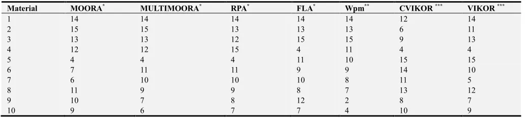
Table 2. Materials ranked by different methods.

Material MOORA* _MULTIMOORA* _RPA* _FLA* _Wpm** _CVIKOR *** _VIKOR ***

1 14 14 14 14 14 12 14

2 15 15 13 13 13 6 11

3 13 13 12 15 15 9 13

4 12 12 15 4 11 4 4

5 4 4 4 11 10 15 15

6 7 11 11 9 9 14 10

7 6 10 10 10 8 11 5

8 11 9 9 8 7 13 12

9 10 7 8 12 2 8 7

Material MOORA* _MULTIMOORA* _RPA* _FLA* _Wpm** _CVIKOR *** _VIKOR ***

11 5 8 6 6 6 5 6

12 8 5 2 5 3 7 8

13 2 2 3 3 12 2 2

14 3 3 1 2 1 1 1

15 1 1 5 1 5 3 3

Sources: *[8]; **[4]; ***[7].

Table 3. Normalized decision matrix for the material selection problem. Criteria

1 2 3 4

Materials

1 0.9832 0.9565 1.0000 0.0000 2 0.9580 0.9565 1.0000 0.0000 3 0.9727 0.9493 1.0000 0.0000 4 0.7234 0.9493 0.2500 0.5000 5 1.0000 1.0000 0.2500 0.5000 6 0.9485 0.9275 0.2500 0.5000 7 0.9252 0.9275 0.2500 0.5000 8 0.8753 0.9831 0.5000 0.2500 9 0.8100 0.9758 0.5000 0.2500 10 0.7997 0.9831 0.5000 0.2500 11 0.7471 0.9807 0.5000 0.2500 12 0.7009 0.9396 0.0000 1.0000 13 0.0537 0.9300 0.2500 0.7500 14 0.3619 0.0000 0.2500 1.0000 15 0.0000 0.9420 0.2500 1.0000

Table 4. Materials ranked by the proposed method.

Material Aggregated performance Rank

1 0.5707 14

2 0.5672 10

3 0.5689 11

4 0.4582 2

5 0.4989 9

6 0.4880 8

7 0.4848 7

8 0.4709 5

9 0.4616 4

10 0.4605 3

11 0.4532 1

Material Aggregated performance Rank

12 0.5707 12

13 0.4713 6

14 0.5707 15

15 0.5707 13

3.2. Intercompany Comparison

Next, the problem of comparing companies as an MODM problem is considered. In a previous study, seven companies

{

1,…, 7

}

A= a a were compared using four criteria

{

c1,…, 4

}

:

C= c profitability

c

₁, productivity

c

₂, market position

c

₃,and reversal debt ratio

c

₄ (note that taking the reversal value of debt ratio as the criterion instead of the debt ratio itself makes all criteria beneficial), [11]. Moreover, the TOPSIS (Technique for Order Preference by Similarity to Ideal Solution) method was considered and different techniques were used for criteria weighting, namely EM (Entropy Measure), CRITIC (CRiteria Importance Through Intercriteria Correlation), SD (Standard Deviation), and MW (Mean Weight), [11]. Note also that the MODM methods are frequently used to develop relevant “composite indicators” for various applications, [12].

The decision matrix for this case study is presented in Table 5. Table 6 lists the companies ranked in descending order obtained using different methods, and Table 7 presents the normalization results.

Table 5. Decision matrix for the company-comparison problem.

# Company Profitability Productivity Market position Reversal debt ratio

PRF PRD MAP RDR

1 2 3 4

1 Company 1 0.12 49469 0.15 1.21

2 Company 2 0.08 34251 0.14 1.23

3 Company 3 0.04 32739 0.09 1.12

4 Company 4 0.16 44631 0.11 1.56

5 Company 5 0.09 33151 0.13 1.09

6 Company 6 0.15 31408 0.07 1.39

7 Company 7 0.13 30654 0.17 1.16

Source: [11]

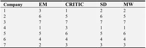
Table 6. Companies ranked by different methods.

Company EM CRITIC SD MW

1 3 1 2 2

2 6 5 6 5

3 7 7 7 7

4 1 3 1 1

5 5 6 5 6

6 4 4 4 4

7 2 3 3 3

Source: [11]

The solution (equilibrium) to the corresponding zero-sum game with mixed strategies is

*

* _,

0, 0, 0.8242, 0, 0, 0.1758, 0

0, 0, 0.7418

( )

. 0 82)

( .25

ξ ζ



= 



= 

*

.

ζ

The results of the corresponding calculations are presented in Table 8.

Table 7. Normalized decision matrix for the company-comparison problem. Criteria

1 2 3 4

Company

1 0.3333 0.0000 0.2000 0.7447 2 0.6667 0.8088 0.3000 0.7021 3 1.0000 0.8892 0.8000 0.9362 4 0.0000 0.2571 0.6000 0.0000 5 0.5833 0.8673 0.4000 1.0000 6 0.0833 0.9599 1.0000 0.3617 7 0.2500 1.0000 0.0000 0.8511

Table 8. Companies ranked by the proposed method.

Company Aggregated performance Rank

1 0.340642 2

2 0.403822 3

3 0.835167 6

4 0.445080 4

5 0.554920 5

6 0.835191 7

7 0.219754 1

Figure 2 shows the solution obtained using the proposed method (dark gray line) in comparison with those obtained using other methods (see Table 6). Note that for the proposed method, with the considered decision matrix and the method for its normalization, the priorities shift in the directions of the market position and reversal debt ratio. In addition, companies 3 and 6 appear to have special status.

Vertical axis: rank; horizontal axis: company (see the main text for an explanation)

Figure 2. Comparison of rankings obtained by different methods for the intercompany comparison problem.

3.3. Employee Selection

Finally, the problem of selecting employees is considered, as investigated in a previous study [13] (note also that application of MODM methods for employee selection problem was also considered recently, e.g. [14]). The alternatives

A

=

{

a

₁

,

…

,

a

₁₇

}

represent 17 people seeking a

position in a company. The criteria

C

=

{

c

₁

,

…

,

c

₁₃

}

represent the results of five different tests: language knowledge, professional knowledge, safety knowledge,

professional skills, and computer skills as well as eight interviews with four managers, which include four face-to-face interviews and four panel interviews; all criteria are beneficial. A total of 16 modifications of TOPSIS are considered, and the corresponding rankings of the 17 persons under consideration are presented. The decision matrix for this case study is presented in Table 9. The applicants ranked in descending order determined using different methods are presented in Table 10; the decision matrix normalization results are presented in Table 11.

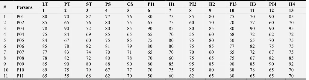
Table 9. Decision matrix for the employee selection problem.

# Persons LT PT ST PS CS PI1 II1 PI2 II2 PI3 II3 PI4 II4

1 2 3 4 5 6 7 8 9 10 11 12 13

1 P01 80 70 87 77 76 80 75 85 80 75 70 90 85

2 P02 85 65 76 80 75 65 75 60 70 70 77 60 70

3 P03 78 90 72 80 85 90 85 80 85 80 90 90 95

4 P04 75 84 69 85 65 65 70 55 60 68 72 62 72

5 P05 84 67 60 75 85 75 80 75 80 50 55 70 75

6 P06 85 78 82 81 79 80 80 75 85 77 82 75 75

7 P07 77 83 74 70 71 65 70 70 60 65 72 67 75

8 P08 78 82 72 80 78 70 60 75 65 75 67 82 85

9 P09 85 90 80 88 90 80 85 95 85 90 85 90 92

10 P10 89 75 79 67 77 70 75 75 80 68 78 65 70

# Persons LT PT ST PS CS PI1 II1 PI2 II2 PI3 II3 PI4 II4

1 2 3 4 5 6 7 8 9 10 11 12 13

12 P12 70 64 65 65 60 60 65 65 75 50 60 45 50 13 P13 95 80 70 75 70 75 75 80 80 65 75 70 75 14 P14 70 80 79 80 85 80 70 75 72 80 70 75 75 15 P15 60 78 87 70 66 70 65 75 70 65 70 60 65 16 P16 92 85 88 90 85 90 95 92 90 85 80 88 90 17 P17 86 87 80 70 72 80 85 70 75 75 80 70 75

Source: [13]

Table 10. Applicants ranked by different methods. Person Methods

M1 M2 M3 M4 M5 M6 M7 M8 M9 M10 M11 M12 M13

1 5 5 5 5 5 5 5 5 5 1 5 1 6

2 14 12 11 14 14 12 11 14 14 14 12 14 12

3 3 3 3 3 3 3 3 3 3 3 3 4 3

4 12 13 13 13 12 13 13 12 12 13 13 13 12 5 11 11 12 11 11 11 12 11 11 11 11 11 11

6 4 4 4 4 4 4 4 4 4 3 4 4 4

7 13 14 14 12 13 14 14 13 13 12 14 11 14

8 8 8 8 8 8 9 9 9 9 9 8 8 8

9 2 2 2 2 2 2 2 2 2 2 1 2 1

10 10 10 10 10 10 10 10 10 10 10 10 10 10 11 16 16 16 16 16 16 16 16 16 17 16 16 16 12 17 17 17 17 17 17 17 17 17 16 16 16 16

13 9 9 9 9 9 8 8 8 8 7 9 7 9

14 6 6 6 6 6 6 6 7 7 8 5 8 5

15 15 15 15 15 15 15 15 15 15 15 15 15 15

16 1 1 1 1 1 1 1 1 1 3 2 3 2

17 7 7 7 7 7 7 7 6 6 3 7 4 6

Source: [13]

The solution (equilibrium) to the corresponding zero-sum game with mixed strategies is

*

*

, , , , , , , , , ,

(0, 0, 0, 0.1989, 0, 0, 0, 0, 0, 0, 0,3899, 0, 4111, 0, 0, 0, 0, 0) 0, 0.0782, 0 0 0 0 0 0 0.5009 0 0 0 0.4209

.

( )

ξ ζ



= 



= 

Therefore, in accordance with the proposed approach, the “proper” performance of the alternatives can be obtained, aggregating their (normalized) performances with weights

*

.

ζ

The results of the corresponding calculations are

presented in Table 12. Figure 3 shows the solution obtained using the proposed method (dark gray line) in comparison with those obtained using other methods (see Table 10). In this example; only three criteria play decisive roles, namely the test of professional knowledge and the face-to-face interviews with managers 2 and 4. Moreover, the aforementioned interviews have roughly the same significance and are greater than that of the test of professional knowledge. In addition, only applicants P04, P11, and P12 appear to have privileged positions.

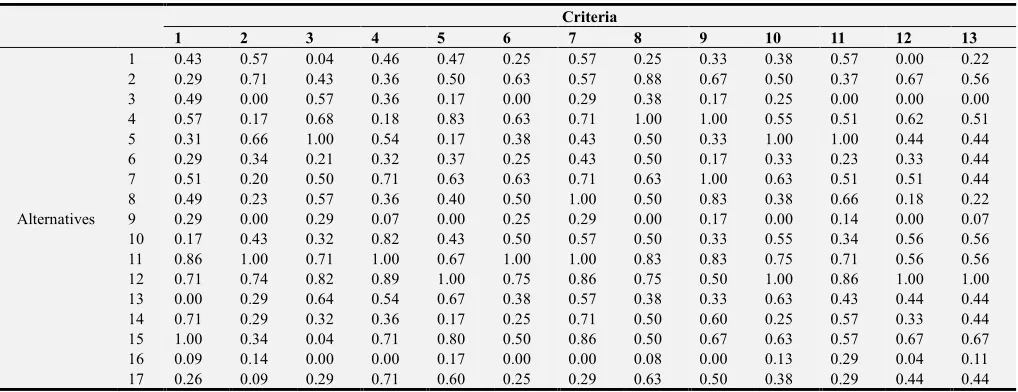
Table 11. Normalized decision matrix for the employee selection problem. Criteria

1 2 3 4 5 6 7 8 9 10 11 12 13

Alternatives

1 0.43 0.57 0.04 0.46 0.47 0.25 0.57 0.25 0.33 0.38 0.57 0.00 0.22

2 0.29 0.71 0.43 0.36 0.50 0.63 0.57 0.88 0.67 0.50 0.37 0.67 0.56

3 0.49 0.00 0.57 0.36 0.17 0.00 0.29 0.38 0.17 0.25 0.00 0.00 0.00

4 0.57 0.17 0.68 0.18 0.83 0.63 0.71 1.00 1.00 0.55 0.51 0.62 0.51

5 0.31 0.66 1.00 0.54 0.17 0.38 0.43 0.50 0.33 1.00 1.00 0.44 0.44

6 0.29 0.34 0.21 0.32 0.37 0.25 0.43 0.50 0.17 0.33 0.23 0.33 0.44

7 0.51 0.20 0.50 0.71 0.63 0.63 0.71 0.63 1.00 0.63 0.51 0.51 0.44

8 0.49 0.23 0.57 0.36 0.40 0.50 1.00 0.50 0.83 0.38 0.66 0.18 0.22

9 0.29 0.00 0.29 0.07 0.00 0.25 0.29 0.00 0.17 0.00 0.14 0.00 0.07

10 0.17 0.43 0.32 0.82 0.43 0.50 0.57 0.50 0.33 0.55 0.34 0.56 0.56

11 0.86 1.00 0.71 1.00 0.67 1.00 1.00 0.83 0.83 0.75 0.71 0.56 0.56

12 0.71 0.74 0.82 0.89 1.00 0.75 0.86 0.75 0.50 1.00 0.86 1.00 1.00

13 0.00 0.29 0.64 0.54 0.67 0.38 0.57 0.38 0.33 0.63 0.43 0.44 0.44

14 0.71 0.29 0.32 0.36 0.17 0.25 0.71 0.50 0.60 0.25 0.57 0.33 0.44

15 1.00 0.34 0.04 0.71 0.80 0.50 0.86 0.50 0.67 0.63 0.57 0.67 0.67

16 0.09 0.14 0.00 0.00 0.17 0.00 0.00 0.08 0.00 0.13 0.29 0.04 0.11

Vertical axis: rank; horizontal axis: applicants (see the main text for an explanation)

Figure 3. Comparison of rankings obtained by different methods for the employee selection problem.

Table 12. Applicants ranked by the proposed method.

Person Aggregated performance Rank

1 0.305179 5

2 0.623621 12

3 0.083485 2

4 0.729443 16

5 0.405417 7

6 0.297361 4

7 0.703616 14

8 0.528829 11

9 0.111545 3

10 0.434315 8

11 0.729443 15

12 0.729443 17

13 0.376379 6

14 0.509954 10

15 0.641351 13

16 0.057937 1

17 0.444227 9

4. Conclusion

As is well known, reaching an agreement about the relative importance of criteria in MODM problems is difficult. Herein, a special game-theoretic approach is proposed to solve this problem. The proposed method leads to a notionally objective weighting method for MODM problems by solving a special two-person zero-sum game. Moreover, the proposed method provides notionally true weights even in the absence of preliminary subjective evaluations.

Further, the proposed method can be applied to decision-making problems with any number of alternatives/criteria and its practical realization is limited only by the capabilities of the solver of the linear programming problem formulated to solve the corresponding zero-sum game. As observed from the solutions of the illustrative examples indicate, the results obtained with the proposed method are quite appropriate and competitive.

References

[1] Marler, R. T., & Arora, J. S. Function-transformation methods for multi-objective optimization. Engineering Optimization, 37(6), 2005, pp. 551-570.

[2] Neumann, Von J. & Morgenstern O. Theory of Games and Economic Behaviour. Princeton University Press, Princeton, NJ, 1944.

[3] Marler, R. T. & Arora, J. S., The weighted sum method for multi-objective optimization: new insights. Structural and multidisciplinary optimization, 41(6), 2010, pp. 853-862. [4] Farag, M. M. Quantitative methods of materials selection. In:

Kutz M, editor. Handbook of materials selection; 2002. [5] Chatterjee, P., Athawale, V. M., and Chakraborty, S. Selection

of materials using compromise ranking and outranking methods. Materials & Design, 30(10), 2009, 4043-4053. [6] Khabbaz, R., Sarfaraz, B., Dehghan Manshadi, A., Abedian,

and R. Mahmudi. A simplified fuzzy logic approach for materials selection in mechanical engineering design. Materials & design 30(3), 2009, pp. 687-697.

[7] Jahan, A., Mustapha, F., Ismail, M. Y., Sapuan, S. M., and Bahraminasab, M. A comprehensive VIKOR method for material selection. Materials & Design, 32(3), 2011, pp. 1215-1221. [8] Karande, P., and Chakraborty, S. Application of

multi-objective optimization on the basis of ratio analysis (MOORA) method for materials selection. Materials & Design 37, 2012, pp. 317-324.

[9] Yazdani, M. New approach to select materials using MADM tools. International Journal of Business and Systems Research, 12(1), 2018, pp. 25-42.

[11] Deng, H., Yeh, C. H., & Willis, R. J. Inter-company comparison using modified TOPSIS with objective weights. Computers & Operations Research, 27(10), 2000, pp. 963-973.

[12] El Gibari, S., Gómez, T. and Ruiz, F. Building composite indicators using multicriteria methods: a review. Journal of Business Economics, 2018, pp. 1-24.

[13] Shih, H. S., Shyur, H. J., & Lee, E. S. An extension of TOPSIS for group decision making. Mathematical and Computer Modelling, 45(7-8), 2007, pp. 801-813.