Perturbed Message Passing for Constraint Satisfaction
Problems
Siamak Ravanbakhsh [email protected]
Russell Greiner [email protected]
Department of Computing Science University of Alberta
Edmonton, AB T6E 2E8, CA
Editor:Alexander Ihler
Abstract
We introduce an efficient message passing scheme for solving Constraint Satisfaction Prob-lems (CSPs), which uses stochastic perturbation of Belief Propagation (BP) and Survey Propagation (SP) messages to bypass decimation and directly produce a single satisfying assignment. Our first CSP solver, calledPerturbed Belief Propagation, smoothly interpo-lates two well-known inference procedures; it starts as BP and ends as a Gibbs sampler, which produces a single sample from the set of solutions. Moreover we apply a similar perturbation scheme to SP to produce another CSP solver, Perturbed Survey Propaga-tion. Experimental results on random and real-world CSPs show that Perturbed BP is often more successful and at the same time tens to hundreds of times more efficient than standard BP guided decimation. Perturbed BP also compares favorably with state-of-the-art SP-guided decimation, which has a computational complexity that generally scales exponentially worse than our method (w.r.t. the cardinality of variable domains and con-straints). Furthermore, our experiments with random satisfiability and coloring problems demonstrate that Perturbed SP can outperform SP-guided decimation, making it the best incomplete random CSP-solver in difficult regimes.
Keywords: constraint satisfaction problem, message passing, belief propagation, survey propagation, Gibbs sampling, decimation
1. Introduction
Probabilistic Graphical Models (PGMs) provide a common ground for recent convergence of themes in computer science (artificial neural networks), statistical physics of disordered systems (spin-glasses) and information theory (error correcting codes). In particular, mes-sage passing methods have been successfully applied to obtain state-of-the-art solvers for Constraint Satisfaction Problems (M´ezard et al., 2002)
The PGM formulation of a CSP defines a uniform distribution over the set of solutions, where each unsatisfying assignment has a zero probability. In this framework, solving a CSP amounts to producing a sample from this distribution. To this end, usually an inference procedure estimates the marginal probabilities, which suggests an assignment to a subset of the most biased variables. This process of sequentially fixing a subset of variables, called
the sense that the procedure’s failure is not a certificate of unsatisfiability. An alternative approach is to use message passing to guide a search procedure that can back-track if a dead-end is reached (e.g., Kask et al., 2004; Parisi, 2003). Here using a branch and bound technique and relying on exact solvers, one may also determine when a CSP is unsatisfiable. The most common inference procedure for this purpose is Belief Propagation (Pearl, 1988). However, due to geometric properties of the set of solutions (Krzakala et al., 2007) as well as the complications from the decimation procedure (Coja-Oghlan, 2011; Kroc et al., 2009), BP-guided decimation fails on difficult instances. The study of the change in the geometry of solutions has lead to Survey Propagation (Braunstein et al., 2002) which is a powerful message passing procedure that is slower than BP (per iteration) but typically remains convergent, even in many situations when BP fails to converge.
Using decimation, or other search schemes that are guided by message passing, usually requires estimating marginals or partition functions, which is harder than producing a single solution (Valiant, 1979). This paper introduces a message passing scheme to eliminate this requirement, therefore also avoiding the complications of applying decimation. Our alternative has advantage over both BP- and SP-guided decimation when applied to solve CSPs. Here we consider BP and Gibbs Sampling (GS) updates as operators—Φ and Ψ respectively—on a set of messages. We then consider inference procedures that are convex combination (i.e., γΨ + (1−γ)Φ) of these two operators. Our CSP solver, Perturbed BP, starts atγ = 0 and ends atγ = 1, smoothly changing from BP to GS, and finally producing a sample from the set of solutions. This change amounts to stochastic biasing the BP messages towards the current estimate of marginals, where this random bias increases in each iteration. This procedure is often much more efficient than BP-guided decimation (BP-dec) and sometimes succeeds where BP-dec fails. Our results on random CSPs (rCSPs) show that Perturbed BP is competitive with SP-guided decimation (SP-dec) in solving difficult random instances.
Since SP can be interpreted as BP applied to an “auxiliary” PGM (Braunstein et al., 2005), we can apply the same perturbation scheme to SP, which we call Perturbed SP. Note that this system, also, does not perform decimation and directly produce a solution (without using local search). Our experiments show that Perturbed SP is often more successful than both SP-dec and Perturbed BP in finding satisfying assignments.
1.1 Factor Graph Representation of CSP
Let x = (x1, x2, . . . , xN) be a tuple of N discrete variables xi ∈ Xi, where each Xi is
the domain of xi. Let I ⊆ N = {1,2, . . . , N} denote a subset of variable indices and
xI={xi|i∈I}be the (sub)tuple of variables inxindexed by the subsetI. Each constraint CI(xI) : Qi∈IXi
→ {0,1} maps an assignment to 1 iff that assignment satisfies that constraint. Then the normalized product of all constraints defines a uniform distribution over solutions
µ(x) , 1
Z
Y
I
CI(xI) (1)
where the partition function Z = P X
Q
ICI(xI) is equal to the number of solutions.1
Notice thatµ(x) is non-zero iff all of the constraints are satisfied—that is x is a solution. With slight abuse of notation we will use probability density and probability distribution interchangeably.
Example 1 (q-COL:) Here, xi ∈ Xi ={1, . . . , q} is a q-ary variable for each i∈ N, and we have M constraints; each constraint Ci,j(xi, xj) = 1−δ(xi, xj) depends only on two variables and is satisfied iff the two variables have different values (colors). Here δ(x, x0) is equal to 1 if x=x0 and 0 otherwise.
This model can be conveniently represented as a bipartite graph, known as a factor graph (Kschischang et al., 2001), which includes two sets of nodes: variable nodes xi, and
constraint (or factor) nodesCI. A variable nodei(note that we will often identify a variable “xi” with its index “i”) is connected to a constraint nodeI if and only if i ∈ I. We will
use∂ to denote the neighbors of a variable or constraint node in the factor graph—that is
∂I ={i | i∈I} (which is the set I) and∂i ={I | i∈I}. Finally we use ∆ito denote the Markov blanket of nodexi (∆i={j∈∂I | I ∈∂i, j6=i}).
The marginal of µ(·) for variablexi is defined as
µ(xi) ,
X
XN \i µ(x)
where the summation above is over all variables but xi. Below, we use bµ(xi) to denote an
estimate of this marginal. Finally, we useS to denote the (possibly empty) set of solutions
S ={x∈ X | µ(x)6= 0}.
Example 2 (κ-SAT:) All variables are binary (Xi={T rue, F alse}) and each clause (con-straint CI) depends on κ=|∂I| variables. A clause evaluates to 0 only for a single assign-ment out of 2κ possible assignment of variables (Garey and Johnson, 1979).
Consider the following 3-SAT problem over 3 variables with 5 clauses
SAT(x) = (¬x1∨ ¬x2∨x3)
| {z }
C1
∧(¬x1∨x2∨x3)
| {z }
C2
∧(x1∨ ¬x2∨x3)
| {z }
C3
∧(¬x1∨x2∨ ¬x3)
| {z }
C4
∧(x1∨ ¬x2∨ ¬x3)
| {z }
C5
. (2)
(a) (b)
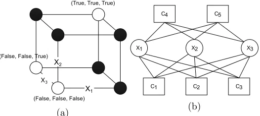
Figure 1: (a) The set of all possible assignments to 3 variables. The solutions to the 3-SAT problem of Equation (2) are in white circles. (b) The factor-graph correspond-ing to the 3-SAT problem of Equation (2). Here each factor prohibits a scorrespond-ingle assignment.
The constraint corresponding to the first clause takes the value 1, except for
x={T rue, T rue, F alse}, in which case it is equal to 0. The set of solutions for this
prob-lem is given by S =
(T rue, T rue, T rue), (F alse, F alse, F alse), (F alse, F alse, T rue) . Figure 1 shows the solutions as well as the corresponding factor graph.2
1.2 Belief Propagation-guided Decimation
Belief Propagation (Pearl, 1988) is a recursive update procedure that sends a sequence of messages from variables to constraints (νi→I) and vice-versa (νI→i)
νi→I(xi) ∝
Y
J∈∂i\I
νJ→i(xi) (3)
νI→i(xi) ∝
X
xI\i∈X∂I\i
CI(xI) Y
j∈∂I\i
νj→I(xj) (4)
where J ∈∂i\I refers to all the factors connected to variable xi, except for factor CI.
Similarly the summation in Equation (4) is over X∂I\i, means we are summing out all xj
that are connected toCI (i.e.,xj s.t. j∈I\i) except for xi.
The messages are typically initialized to a uniform or a random distribution. This re-cursive update of messages is usually performed until convergence—i.e., until the maximum change in the value of all messages, from one iteration to the next, is negligible (i.e., below some small ). At any point during the updates, the estimated marginal probabilities are given by
b
µ(xi) ∝ Y J∈∂i
νJ→i(xi). (5)
In a factor graph without loops, each BP message summarizes the effect of the (sub-tree that resides on the) sender-side on the receiving side.
Example 3 Applying BP to the 3-SAT problem of Equation (2) takes 20 iterations to converge (i.e., for the maximum change in the marginals to be below = 10−9). Here the message, νC1→1(x1), fromC1 to x1 is
νC1→1(x1) ∝
X
x2,3
C1(x1,2,3)ν2→C1(x2)ν3→C1(x3)
and similarly, the message in the opposite direction, ν1→C1(x1), is defined as
ν1→C1(x1) ∝ νC2→1(x1)νC3→1(x1)νC4→1(x1)νC5→1(x1).
Here BP gives us the following approximate marginals: µb(x1 =T rue) =µb(x2=T rue) =
.319andµb(x3 =T rue) =.522. From the set of solutions, we know that the correct marginals
are µb(x1 =T rue) = bµ(x2 = T rue) = 1/3 and µb(x3 = T rue) = 2/3. The error of BP is
caused by influential loops in the factor-graph of Figure 1(b). Here the error is rather small; it can be arbitrarily large in some instances or BP may not converge at all.
The time complexity of BP updates of Equation (3) and Equation (4), for each of the messages exchanged between i and I, are O(|∂i| |Xi|) and O(|XI|) respectively. We may
reduce the time complexity of BP by synchronously updating all the messagesνi→I ∀I ∈∂i
that leave node i. For this, we first calculate the beliefs µb(xi) using Equation (5) and
produce eachνi→I using
νi→I(xi) ∝ b µ(xi)
νI→i(xi)
. (6)
Note than we can substitute Equation (4) into Equation (3) and Equation (5) and only keep variable-to-factor messages. After this substitution, BP can be viewed as a fixed-point iteration procedure that repeatedly applies the operator
Φ({νi→I}),{Φi→I({νj→J}j∈∆i,J∈∂i\I})}i,I∈∂ito the set of messages in hope of reaching a
fixed point—that is
νi→I(xi) ∝
Y
J∈∂i\I
X
X∂J\i
CJ(xJ)
Y
j∈∂J\i
νj→J(xj) , Φi→I({νj→J}j∈∆i,J∈∂i\I)(xi) (7)
and therefore Equation (5) becomes
b
µ(xi) ∝
Y
I∈∂i
X
X∂I\i
CI(xI)
Y
j∈∂I\i
νj→I(xj) (8)
where Φi→I denotes individual message update operators. We let operator Φ(.) denote the
1.2.1 Decimation
The decimation procedure can employ BP (or SP) to solve a CSP. We refer to the cor-responding method as BP-dec (or SP-dec). After running the inference procedure and obtaining µb(xi), ∀i, the decimation procedure uses a heuristic approach to select the most
biased variables (or just a random subset) and fixes these variables to their most biased values (or a randomxib ∼µb(xi)). If it selects a fractionρ of remaining variables to fix after
each convergence, this multiplies an additional log1
ρ(N) to the linear (in N) cost
3 for each iteration of BP (or SP). The following algorithm 1 summarizes BP-dec with a particular scheduling of updates:
input : factor-graph of a CSP
output: a satisfying assignment x∗ if an assignment was found. unsatisfied
otherwise
1 initialize the messages
2 N ← Ne (set of all variable indices)
3 while Ne is not empty do// decimation loop
4
5 repeat// BP loop
6
7 foreachi∈Ne do
8 calculate messages{νI→i}I∈∂i using Equation (4)
9 if {νI→i}I∈∂i are contradictory then return:unsatisfied
10 calculate marginalµb(xi) using Equation (5)
11 calculate messages{νi→I}I∈∂i using Equation (3) or Equation (6)
12 untilconvergence
13 selectB ⊆Ne using{ b
µ(xi)}i∈ e
N 14 fixx∗j ←argx
jmaxµb(xj) ∀j∈ B
15 reduce the constraints{CI}I∈∂j for everyj∈ B return:x∗ = (x∗1, . . . , x∗N)
Algorithm 1:Belief Propagation-guided Decimation (BP-dec)
The condition of line 9 is satisfied iff the product of incoming messages to node i is 0 for all xi ∈ Xi. This means that neighboring constraints have strict disagreement about
the value of xi and the decimation has found a contradiction. This contradiction can happen because, either (I) there is no solution for the reduced problem even if the original problem had a solution, or (II) the reduced problem has a solution but the BP messages are inaccurate.
Example 4 To apply BP-dec to previous example, we first calculate BP marginals, as shown in the example above. Here bµ(x1) and µb(x2) have the highest bias. By fixing the 3. Assuming the number of edges in the factor graph are in the order ofN. In general, using synchronous update of Equation (6) and assuming a constant factor cardinality, |∂I|, the cost of each iteration is
value ofx1 toF alse, the SAT problem of Equation (2) collapses to
SAT(x{2,3})|x1=F alse = (¬x2∨x3)∧(¬x2∨ ¬x3).
BP-dec applies BP again to this reduced problem, which give µb(x2 =T rue) =.14 (note
here that µ(x2 = T rue) = 0) and µb(x3 = T rue) = 1/2. By fixing x2 to F alse, another
round of decimation yields a solution x∗ = (F alse, F alse, T rue).
1.3 Gibbs Sampling as Message Update
Gibbs Sampling (GS) is a Markov Chain Monte Carlo (MCMC) inference procedure (An-drieu et al., 2003) that can produce a set of samples xb[1], . . . ,xb[L] from a given PGM. We
can then recover the marginal probabilities, as empirical expectations
b
µL(xi) ∝
1
L L
X
n=1
δ(bx[n]i, xi). (9)
Our algorithm only considers a single particlexb=xb[1]. GS starts from a random initial statexb
(t=0) and at each time-step t, updates each b
xi by sampling from:
b
x(it) ∼ µ(xi) ∝
Y
I∈∂i
CI(xi,xb (t−1)
∂I\i ) (10)
If the Markov chain satisfies certain basic properties (Robert and Casella, 2005), x(∞)i
is guaranteed to be an unbiased sample from µ(xi) and therefore our marginal estimate,
b
µL(xi), becomes exact as L→ ∞.
In order to interpolate between BP and GS, we establish a correspondence between a particle in GS and a set of variable-to-factor messages—i.e., bx⇔ {νi→I(.)}i,I∈∂i. Here all
the messages leaving variablexi are equal to aδ-function defined based onxib
νi→I(xi) = δ(xi,bxi) ∀I ∈∂i.
We define the random GS operator Ψ = {Ψi}i and rewrite the GS update of
Equa-tion (10) as
νi→I(xi) , Ψi({νj→J(xj)}j∈∆i,J∈∂i)(xi) = δ(xbi, xi) (11)
wherexib is sampled from
b
xi ∼ µb(xi) ∝ Y
J∈∂i
CI(xi,bx∂I\i)
∝ Y
I∈∂i
X
X∂I\i
CI(xI) Y
j∈∂I\i
νj→I(xj). (12)
2. Perturbed Belief Propagation
Here we introduce an alternative to decimation that does not require repeated application of inference. The idea is to use a linear combination of BP and GS operators (Equation 7 and Equation 11) to update the messages
Γ({νi→I}),γ Ψ({νi→I}) + (1−γ)Φ({νi→I}).
The Perturbed BP operator Γ ={Γi→I}i,I∈∂i updates each message by calculating the
outgoing message according to BP and GS operators and linearly combines them to get the final message. During T iterations of Perturbed BP, the parameter γ is gradually and linearly changed from 0 towards 1. Algorithm 2 below summarizes this procedure.
input : factor graph of a CSP, number of iterations T
output: a satisfying assignment x∗ if an assignment was found. unsatisfied
otherwise
1 initialize the messages
2 γ ←0
3 N ← Ne (set of all variable indices)
4 for t= 1 toT do
5 foreach variable xi do
6 calculateνI→i using Equation (4)∀I ∈∂i
7 if {νI→i}I∈∂i are contradictory then return:unsatisfied
8 calculate marginals bµ(xi) using Equation (12)
9 calculate BP messagesνi→I using Equation (3) or Equation (6) ∀I ∈∂i.
10 samplexbi∼bµ(xi)
11 combine BP and Gibbs sampling messages:
νi→I ← γ νi→I + (1−γ) δ(xi,bxi)
12 γ←γ+ T1−1
return:x∗ ={x∗1, . . . , x∗N}
Algorithm 2:Perturbed Belief Propagation
In step 7, if the product of incoming messages is 0 for all xi ∈ Xi for some i, different
neighboring constraints have strict disagreement aboutxi; therefore this run of Perturbed BP will not be able to satisfy this CSP. Since the procedure is inherently stochastic, if the CSP is satisfiable, re-application of the same procedure to the problem may avoid this specific contradiction.
2.1 Experimental Results on Benchmark CSP
This section compares the performance of BP-dec and Perturbed BP on benchmark CSPs. We considered CSP instances from XCSP repository (Roussel and Lecoutre, 2009; Lecoutre, 2013), without global constraints or complex domains.4
We used a convergence threshold of = .001 for BP and terminated if the threshold was not reached after T = 10×210 = 10,240 iterations. To perform decimation, we sort the variables according to their bias and fix ρ fraction of the most biased variables in each iteration of decimation. This fraction, ρ, was initially set to 100%, and it was divided by 2 each time BP-dec failed on the same instance. BP-dec was repeatedly applied using the reducedρ, at most 10 times, unless a solution was reached (that isρ=.1% at final attempt). For Perturbed BP, we set T = 10 at the starting attempt, which was increased by a factor of 2 in case of failure. This was repeated at most 10 times, which means Perturbed BP used T = 10,240 at its final attempt. Note that Perturbed BP at most uses the same number of iterations as the maximum iterations per single iteration of decimation in BP-dec.
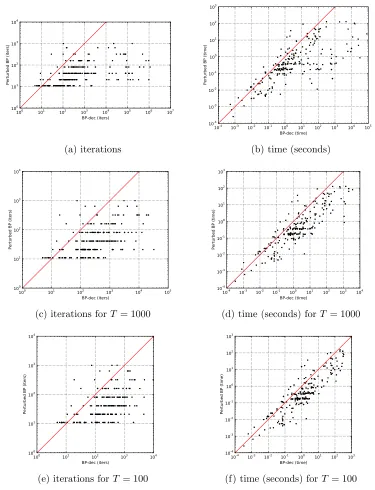
Figure 2(a,b) compares the time and iterations of BP-dec and Perturbed BP for success-ful attempts where both methods satisfied an instance. The result for individual problem-sets is reported in the appendix.
Empirically, we found that Perturbed BP both solved (slightly) more instances than BP-dec (284 vs 253), and was (hundreds of times) more efficient: while Perturbed BP required only 133 iterations on average, BP-dec required an average of 41,284 iterations for successful instances.
We also ran BP-dec on all the benchmarks with maximum number of iterations set to
T = 1000 and T = 100 iterations. This reduced the number of satisfied instances to 249 for T = 1000 and 247 for T = 100, but also reduced the average number of iterations to 1570 and 562 respectively, which are still several folds more expensive than Perturbed BP. Figure 2(c-f) compare the time and iterations used by BP-dec in these settings with that of Perturbed BP, when both methods found a satisfying assignment. See the appendix for a more detailed report on these results.
3. Critical Phenomena in Random CSPs
Random CSP (rCSP) instances have been extensively used in order to study the properties of combinatorial problems (Mitchell et al., 1992; Achioptas and Sorkin, 2000; Krzakala et al., 2007) as well as in analysis and design of algorithms (e.g., Selman et al., 1994; M´ezard et al., 2002). Random CSPs are closely related to spin-glasses in statistical physics (Kirkpatrick and Selman, 1994; Fu and Anderson, 1986). This connection follows from the fact that the Hamiltonian of these spin-glass systems resembles the objective functions in many combinatorial problems, which decompose to pairwise (or higher order) interactions, allowing for a graphical representation in the form of a PGM. Here message passing methods, such as belief propagation (BP) and survey propagation (SP), provide consistency conditions on locally tree-like neighborhoods of the graph.
The analogy between a physical system and computational problem extends to their critical behavior where computation relates to dynamics (Ricci-Tersenghi, 2010). In
100 101 102 103 104 105 106 107 BP-dec (iters) 100 101 102 103 104
Perturbed BP (iters)
(a) iterations
10-4 10-3 10-2 10-1 100 101 102 103 104 105 BP-dec (time) 10-4 10-3 10-2 10-1 100 101 102 103
Perturbed BP (time)
(b) time (seconds)
100 101 102 103 104 105 BP-dec (iters) 100 101 102 103 104
Perturbed BP (iters)
(c) iterations forT = 1000
10-4 10-3 10-2 10-1 100 101 102 103 104 BP-dec (time) 10-4 10-3 10-2 10-1 100 101 102 103
Perturbed BP (time)
(d) time (seconds) forT = 1000
100 101 102 103 104 BP-dec (iters) 100 101 102 103 104
Perturbed BP (iters)
(e) iterations forT = 100
10-4 10-3 10-2 10-1 100 101 102 103 BP-dec (time) 10-4 10-3 10-2 10-1 100 101 102 103
Perturbed BP (time)
(f) time (seconds) forT = 100
puter science, this critical behavior is related to the time-complexity of algorithms employed to solve such problems, while in spin-glass theory this translates to dynamics of glassy state, and exponential relaxation times (M´ezard et al., 1987). In fact, this connection has been used to attempt to prove the conjecture that P is not equal toN P (Deolalikar, 2010).
Studies of rCSP, as a critical phenomena, focus on the geometry of the solution space as a function of the problem’s difficulty, where rigorous (e.g., Achlioptas and Coja-Oghlan, 2008; Cocco et al., 2003) and non-rigorous (e.g., cavity method of M´ezard and Parisi, 2001, 2003) analyses have confirmed the same geometric picture.
When working with large random instances, a scalar α associated with a problem in-stance, a.k.a. control parameter—for example, the clause to variable ratio in SAT—can characterize that instance’s difficulty (i.e., larger control parameter corresponds to a more difficult instance) and in many situations it characterizes a sharp transition from satisfia-bility to unsatisfiasatisfia-bility (Cheeseman et al., 1991).
Example 5 (Random κ-SAT) Randomκ-SAT instance withN variables and M =αN constraints are generated by selecting κ variables at random for each constraint. Each constraint is set to zero (i.e., unsatisfied) for a single random assignment (out of2κ). Here α is the control parameter.
Example 6 (Random q-COL) The control parameter for a random q-COL instances with N variables and M constraints is its average degree α = 2NM. We consider Erd˝ os-R´eny random graphs and generate a random instance by sequentially selecting two distinct variables out ofN at random to generate each ofM edges. For largeN, this is equivalent to selecting each possible factor with a fixed probability, which means the nodes have Poisson degree distribution P(|∂i|=d)∝e−ααd.
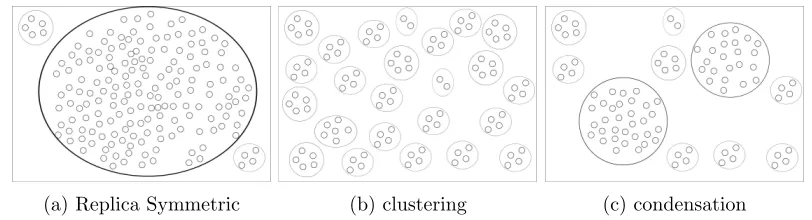
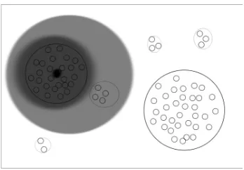
While there are tight bounds for some problems (e.g., Achlioptas et al., 2005), finding the exact location of this transition for different CSPs is still an open problem. Besides transition to unsatisfiability, these analyses has revealed several other (phase) transitions (Krzakala et al., 2007). Figure 3(a)-(c) shows how the geometry of the set of solutions changes by increasing the control parameter.
Here we enumerate various phases of the problem for increasing values of the control parameter: (a) In the so-called Replica Symmetric (RS) phase, the symmetries of the set of solutions (a.k.a. ground states) reflect the trivial symmetries of problem w.r.t. variable domains. For example, forq-COL the set of solutions is symmetric w.r.t. swapping all red and blue assignment. In this regime, the set of solutions form a giant cluster (i.e., a set of neighboring solutions), where two solutions are considered neighbors when their Ham-ming distance is one (Achlioptas and Coja-Oghlan, 2008) or non-divergent with number of variables (M´ezard and Parisi, 2003). Local search methods (e.g., Selman et al., 1994) and BP-dec can often efficiently solve random CSPs that belong to this phase.
(b) In clustering or dynamical transition (1dRSB5), the set of solutions decomposes into an exponential number of distant clusters. Here two clusters are distant if the Ham-ming distance between their respective members is divergent (e.g., linear) in the number
(a) Replica Symmetric (b) clustering (c) condensation
Figure 3: A 2-dimensional schematic view of how the set of solutions of CSP varies as we increase the control parameter α from (a) replica symmetric phase to (b) clus-tering phase to (c) condensation phase. Here small circles represent solutions and the bigger circles represent clusters of solutions. Note that this view is very simplistic in many ways; for example, the total number of solutions and the size of clusters should generally decrease from (a) to (c).
of variables. (c) In the condensation phase transition (1sRSB6), the set of solutions con-denses into a few dominant clusters. Dominant clusters have roughly the same number of solutions and they collectively contain almost all of the solutions. While SP can be used even within the condensation phase, BP usually fails to converge in this regime. However each cluster of solutions in the clustering and condensation phase is a valid fixed-point of BP, which is called a “quasi-solution” of BP. (d) A rigidity transition (not included in Figure 3) identifies a phase in which a finite portion of variables are fixed within dominant clusters. This transition triggers an exponential decrease in the total number of solutions, which leads to (e) unsatisfiability transition.7 This rough picture summarizes first order Replica Symmetry Breaking’s (1RSB) basic assumptions (M´ezard and Montanari, 2009).
From a geometric perspective, the intuitive idea behind Perturbed BP, is to perturb the messages towards a solution. However, in order to achieve this, we need to initialize the messages to a proper neighborhood of a solution. Since these neighborhoods are not initially known, we resort to stochastic perturbation of messages to make local marginals more biased towards a subspace of solutions. This continuous perturbation of all messages is performed in a way that allows each BP message to re-adjust itself to the other perturbations, more and more focusing on a random subset of solutions.
3.1 1RSB Postulate and Survey Propagation
Large random graphs are locally tree-like, which means the length of short loops are typically in the order of log(N) (Janson et al., 2001). This ensures that, in the absence of long-range correlations, BP is asymptotically exact, as the set of messages incoming to each node or factor are almost independent. Although BP messages remain uncorrelated until the condensation transition (Krzakala et al., 2007), the BP equations do not completely characterize the set of solutions after the clustering transition. This inadequacy is indicated
6. 1sRSB is short for 1st order static Replica Symmetry Breaking.
by the existence of a set of several valid fixed points (rather than a unique fixed-point) for BP, each of which corresponds to a quasi-solution. For a better intuition, consider the cartoons of Figures 3(b) and (c). During the clustering phase (b),xi andxj (corresponding
to thexand yaxes) are not highly correlated, but they become correlated during and after condensation (c). This correlation between variables that are far apart in the PGM results in correlation between the BP messages. This violates BP’s assumption that messages are uncorrelated, which results in BP’s failure in this regime.
1RSB’s approach to incorporating this clustering of solutions into the equilibrium condi-tions is to define a new Gibbs measure over clusters. Lety⊂ S denote a cluster of solutions and Y be the set of all such clusters. The idea is to treat Y the same as we treatedX, by defining a distribution
µ(y) ∝ |y|m ∀y∈ Y (13)
where m ∈ [0,1], called the Parisi parameter (M´ezard et al., 1987), specifies how each cluster’s weight depends on its size. This implicitly defines a distribution overX
µ(x) ∝ X
y3x
µ(y) (14)
N.b.,m= 1 corresponds to the original distribution (Equation (1)).
Example 7 Going back to our simple 3-SAT example, y(1) = {(T rue, T rue, T rue)} and y(2) = {(F alse, F alse, F alse), (F alse, F alse, T rue)} are two clusters of solutions. Using m= 1, we have
µ({{T rue, T rue, T rue}}) = 1/3 and µ({{F alse, F alse, F alse},{F alse, F alse, T rue}}) = 2/3. This distribution over clusters reproduces the distribution over solutions—i.e.,µ(x) = 1/3∀x∈ S. On the other hand, usingm= 0, produces a uniform distribution over clusters, but it does not give us a uniform distribution over the solutions.
This meta-construction for µ(y) can be represented using an auxiliary PGM. One may use BP to find marginals over this PGM; here BP messages are distributions over all BP messages in the original PGM, as each cluster is a fixed-point for BP. This requirement to represent a distribution over distributions makes 1RSB practically intractable. In general, each original BP message is a distribution overXi and it is difficult to define a distribution over this infinite set. However this simplifies if the original BP messages can have limited values. Fortunately if we apply max-product BP to solve a CSP, instead of sum-product BP (of Equations (3) and (4)), the messages can have a finite set of values.
Max-Product BP: Our previous formulation of CSP was using sum-product BP. In general, max-product BP is used to find the Maximum a Posteriori (MAP) assignment in a PGM, which is a single assignment with the highest probability. In our PGM, the MAP assignment is a solution for the CSP. The max-product update equations are
ηi→I(xi) = QJ∈∂i\IηJ→i(xi) = Λi→I( {ηJ→i}J∈∂i\I )(xi) (15)
ηI→i(xi) = maxX∂I\iCI(xI)
Q
j∈∂I\iηj→I(xj) = ΛI→i( {ηj→I}j∈∂I\i )(xi) (16)
b
µ(xi) = Q
where Λ = {Λi→I,ΛI→i}i,I∈∂I is the max-product BP operator and Λi represents the
marginal estimate as a function of messages. Note that here messages and marginals are not distributions. We initialize νi→I(xi) ∈ {0,1}, ∀I, i ∈ ∂I, xi ∈ Xi. Because of the way
constraints and update equations are defined, at any point during the updates we have
νi→I(xi) ∈ {0,1}. This is also true for bµ(xi). Here any of νi→I(xi) = 1, νI→i(xi) = 1
or µb(xi) = 1, shows that value xi is allowed according to a message or marginal, while
0 forbids that value. Note that µb(xi) = 0 ∀xi ∈ Xi iff no solution was found, because
the incoming messages were contradictory. The non-trivial fixed-points of max-product BP define quasi-solutions in 1RSB phase, and therefore define clusters y.
Example 8 If we initialize all messages to 1 for our simple 3-SAT example, the final marginals over all the variables are equal to 1, allowing all assignments for all variables. However beside this trivial fixed-point, there are other fixed points that correspond to two clusters of solutions.
For example, considering the cluster {(F alse, F alse, F alse),(F alse, F alse, T rue)}, the following{ηi→I} (and their corresponding {ηI→i} define a fixed-point for max-product BP:
η1→I(T rue) =µb1(T rue) = 0 η1→I(F alse) =bµ1(F alse) = 1 ∀I ∈∂1
η2→I(T rue) =µb2(T rue) = 0 η2→I(F alse) =bµ2(F alse) = 1 ∀I ∈∂2
η3→I(T rue) =µb3(T rue) = 1 η3→I(F alse) =bµ3(F alse) = 1 ∀I ∈∂3
Here the messages indicate the allowed assignments within this particular cluster of solu-tions.
3.1.1 Survey Propagation
Here we define the 1RSB update equations over max-product BP messages. We skip the explicit construction of the auxiliary PGM that results in SP update equations, and confine this section to the intuition offered by SP messages. Braunstein et al. (2005) and M´ezard and Montanari (2009) give details on the construction of the auxiliary-PGM. Ravanbakhsh and Greiner (2014) present an algebraic perspective on SP. Maneva et al. (2007) provide a different view on the relation of BP and SP for the satisfiability problem and Kroc et al. (2007) present empirical study of SP as applied to SAT.
Let Yi = 2|Xi| be the power-set8 of Xi. Each max-product BP message can be seen as
a subset of Xi that contains the allowed states. Therefore Yi as its power-set contains all
possible max-product BP messages. Each messageνi→I : Yi →[0,1] in the auxiliary PGM
defines adistribution over original max-product BP messages.
Example 9 (3-COL) Xi={1,2,3} is the set of colors and
Yi ={{},{1},{2},{3},{1,2},{2,3},{1,3},{1,2,3}}. Here yi ={} corresponds to the case where none of the colors are allowed.
Applying sum-product BP to our auxiliary PGM gives entropic SP(m) updates as:
νi→I(yi)∝ |yi|m
X
{ηJ→i}J∈∂i\I
δ(yi,Λi→I({ηJ→i}J∈∂i\I))
Y
J∈∂i\I
νJ→i(ηJ→i) (18)
νI→i(yi)∝ |yi|m
X
{ηj→I}j∈∂I\i
δ(yi,ΛI→i({ηj→I}j∈∂I\i))
Y
j∈∂I\i
νj→I(ηj→I) (19)
νi→I({}) := νI→i({}) := 0 ∀i, I∈∂i (20)
where the summations are over all combinations of max-product BP messages. Here the
δ-function ensures that only the set of incoming messages that satisfy the original BP equations make contributions. Since we only care about the valid assignments andyi={}
forbids all assignments, we ignore its contribution (Equation 20).
Example 10 (3-SAT) Consider the SP message ν1→C1(y1) in the factor graph of
Fig-ure 1b. Here the summation in Equation (18) is over all possible combinations of incoming max-product BP messages ηC2→1, . . . , ηC5→1. Since each of these messages can assume one
of the three valid values—e.g., ηC2→1(x1)∈ { {T rue},{F alse},{T rue, F alse} }—for each
particular assignment of y1, a total of |{{T rue},{F alse},{T rue, F alse}}||∂1\C1|= 34
pos-sible combinations are enumerated in the summations of Equation (18). However only the combinations that form a valid max-product message update have non-zero contribution in calculating ν1→C1(y1). These are basically the messages that appear in a max-product fixed
point as discussed in Example 8.
Each of original messages corresponds to a different sub-set of clusters and m (from Equation (13)) controls the effect of each cluster’s size on its contribution. At any point, we can use these messages to estimate the marginals ofµb(y) defined in Equation (13) using
b
µ(yi) ∝ |yi|m
X
{ηJ→i}J∈∂i
δ(yi, Λi( {ηJ→i}J∈∂i) )
Y
J∈∂i
νJ→i(ηJ→i). (21)
This also implies a distribution over the original domain, which we slightly abuse nota-tion to denote by
b
µ(xi) ∝
X
yi3xi
b
µ(yi). (22)
The term SP usually refers to SP(0)—that is m = 0—where all clusters, regardless of their size, contribute the same amount to µ(y). Now that we can obtain an estimate of marginals, we can employ this procedure within a decimation process to incrementally fix some variables. Here either µb(xi) or µb(yi) can be used by the decimation procedure to fix
the most biased variables. In the former case, a variable yi is fixed to y∗i = {x∗i} when x∗i = argximaxµb(xi). In the latter case, y
∗
i = argyimaxµb(yi). Here we use SP-dec(S) to
refer to the former procedure (that uses µb(xi) to fix variables to a single value) and use
can choose to fix a cluster toyi={T rue, F alse}in addition to the options ofyi ={T rue}
and yi = {F alse}, available to SP-dec(S). However, for larger domains (e.g., q-COL),
SP-dec(C) has a clear advantage. For example in 3-COL, SP-dec(C) may choose to fix a cluster to yi ={1,2} while SP-dec(S) can only choose between yi ∈ {{1},{2},{3}}. This
significant difference is also reflected in their comparative success-rate on q-COL.9 (See Table 1 in Section 3.3.)
During the decimation process, usually after fixing a subset of variables, the SP marginals
b
µ(xi) become uniform, indicating that clusters of solutions have no preference over particu-lar assignments of the remaining variables. The same happens when we apply SP to random instances in RS phase. At this point (a.k.a. paramagnetic phase), a local search method or BP-dec can often efficiently find an assignment to the variables that are not yet fixed by decimation. Note that both SP-dec(C) and SP-dec(S) switch to local search as soon as all
b
µ(xi) become close to uniform.
The computational complexity of each SP update of Equation (19) isO(2|Xi|−1)|∂I|as for
each particular valueyi, SP needs to consider every combination of incoming messages, each
of which can take 2|Xi|values (minus the empty set). Similarly, using a naive approach the
cost of update of Equation (18) isO(2|Xi|−1)|∂i|. However by considering incoming messages
one at a time, we can perform the same exact update in O(|∂i|22|Xi|). In comparison to
the cost of BP updates, we see that SP updates are substantially more expensive for large
|Xi|and |∂I|.10
3.2 Perturbed Survey Propagation
The perturbation scheme that we use for SP is similar to what we did for BP. Let
Φi→I( {νj→J}j∈∆i,(J∈∂i)\I) ) denote the update operator for the message from variableyi
to factor CI. This operator is obtained by substituting Equation (19) into Equation (18) to get a single SP update equation. LetΦ({νi→I}i,I∈∂i) denote the aggregate SP operator,
which appliesΦi→I to update each individual message.
We perform Gibbs sampling from the “original” domain X using the implicit marginal of Equation (22). We denote this random operator by Ψ={Ψi}i, defined by
νi→I(yi) = Ψi({νj→J}j∈∆i,J∈∂i ) , δ(yi,{bxi}) wherebxi ∼µb(xi)
where the second argument of theδ-function is a singleton set, containing a sample from the estimate of marginal. Now, define the Perturbed SP operator as the convex combination of SP and either of the GS operator above:
Γ({νi→I}) , γΨ({νi→I}) + (1−γ)Φ({νi→I}).
Similar to perturbed BP, during iterations of Perturbed SP, γ is gradually increased from 0 to 1. If perturbed SP reaches the final iteration, the samples from the implicit
9. Previous applications of SP-dec toq-COL by Braunstein et al. (2003) used a heuristic for decimation that is similar SP-dec (C).
10. Note that our representation of distributions is over-complete—that is we are not using the fact that the distributions sum to one. However even in their more compact forms, for general CSPs, the cost of each SP update remains exponentially larger than that of BP (in|Xi|,|∂I|). However if the factors are sparse
marginals represent a satisfying assignment. The advantage of this scheme to SP-dec is that perturbed SP does not require any further local search. In fact we may apply Γ to CSP instances in the RS phase as well, where the solutions form a single giant cluster. In contrast, applying SP-dec, to these instances simply invokes the local search method.
To demonstrate this, we applied Perturbed SP(S) to benchmark CSP instances of Table 2 in which the maximum number of elements in the factor was less than 10. Here Perturbed SP(S) solved 80 instances out of 202 cases, while Perturbed BP solved 78 instances.
3.3 Experiments on random CSP
We implemented all the methods above for general factored CSP using the libdai code base (Mooij, 2010). To our knowledge this is the first general implementation of SP and SP-dec. Previous applications of SP-dec toκ-SAT andq-COL (Braunstein et al., 2003; Mulet et al., 2002; Braunstein et al., 2002) were specifically tailored to just one of those problems.
Here we report the results onκ-SAT forκ∈ {3,4}andq-COL forq∈ {3,4,9}. We used the procedure discussed in the examples of Section 3 to produce 100 random instances with
N = 5,000 variables for each control parameter α. We report the probability of finding a satisfying assignment for different methods (i.e., the portion of 100 instances that were satisfied by each method). For coloring instances, to help decimation, we break the initial symmetry of the problem by fixing a single variable to an arbitrary value.
For BP-dec and SP-dec, we use a convergence threshold of = .001 and fix ρ = 1% of variables per iteration of decimation. Perturbed BP and Perturbed SP use T = 1000 iterations. Decimation-based methods use a maximum ofT = 1000 iterations per iteration of decimation. If any of the methods failed to find a solution in the first attempt, T was increased by a factor of 4 at most 3 times (so in the final attempt: T = 64,000). To avoid blow-up in run-time, for BP-dec and SP-dec, only the maximum iteration, T, during the first iteration of decimation, was increased (this is similar to the setting of Braunstein et al. (2002) for SP-dec). For both variations of SP-dec (see Section 3.1.1), after each decimation step, if maxi,xiµ(xi)−
1
|Xi| < .01 we consider the instance para-magnetic, and run BP-dec
(with T = 1000,=.001 and ρ= 1%) on the simplified instance.
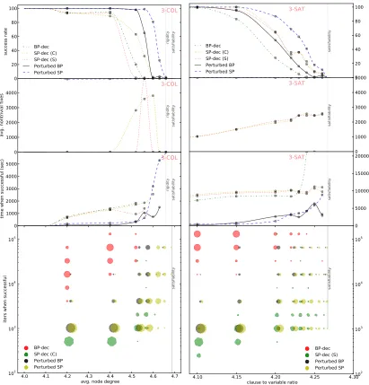
Figure 4(first row) visualizes the success rate of different methods on 100 instances of 3-SAT (right) and 3-COL (left). Figure 4(second row) reports the number of variables that are fixed by SP-dec(C) and (S) before calling BP-dec as local search. The third row shows the average amount of time that is used to find a satisfying solution. This does not include the failed attempts. For SP-dec variations, this time includes the time used by local search. The final row of Figure 4 shows the number of iterations used by each method at each level of difficulty over the successful instances. Here the area of each disk is proportional to the frequency of satisfied instances with that particular number of iterations for each control parameter and inference method11.
Here we make the following observations:
• Perturbed BP is much more effective than BP-dec, while remaining ten to hundreds of times more efficient.
• As the control parameter grows larger, the chance of requiring more iterations to satisfy the instance increases for all methods.
• Although computationally very inefficient, BP-dec is able to find solutions for in-stances with larger control parameters than suggested by previous results (e.g., M´ezard and Montanari, 2009).
• For many instances where SP-dec(C) and (S) use few iterations, the variables are fixed to a trivial cluster yi = Xi, which allows all assignments. This is particularly
pronounced for 3-COL, where up to α = 4.4 the non-trivial fixes remains zero and therefore the success rate up to this point is solely due to BP-dec.
• While for 3-SAT, SP-dec(C) and SP-dec(S) have a similar performance, for 3-COL, SP-dec(C) significantly outperforms SP-dec(S).
Table 1 reports the success-rate as well as the average of total iterations in thesuccessful
attempts of each method. Here the number of iterations for SP-dec(C) and (S) is the sum of iterations used by the method and the following local search. We observe that Perturbed BP can solve most of the easier instances using only T = 1000 iterations (e.g., see Perturb BP’s result for 3-SAT at α= 4.1, 3-COL atα= 4.2 and 9-COL atα= 33.4).
Table 1 also supports our speculation in Section 3.1.1 that SP-dec(C) is in general preferable to SP-dec(S), in particular when applied to the coloring problem.
The most important advantage of Perturbed BP over SP-dec and Perturbed SP is that Perturbed BP can be applied to instances with large factor cardinality (e.g., 10-SAT) and large variable domains (e.g., 9-COL). For example for 9-COL, the cardinality of each SP message is 29 = 512, which makes SP-dec and Perturbed SP impractical. Here BP-dec is not even able to solve a single instance around the dynamical transition (as low asα= 33.4) while Perturbed BP satisfies all instances up to α = 34.1.12 Besides the experimental re-sults reported here, we have also used perturbed BP to efficiently solve other CSPs such as K-Packing, K-set-cover and clique-cover within the context of min-max inference (Ravan-bakhsh et al., 2014).
3.4 Discussion
It is easy to check that, for m = 1, SP updates produce sum-product BP messages as an average case; that is, the SP updates (equations 18, 19) reduce to that of sum-product BP (equations 3, 4) where
νi→I(xi) ∝
X
yi3xi
νi→I(yi)
This suggests that the BP equation remains correct wherever SP(1) holds, which has lead to the belief that BP-dec should perform well up to the condensation transition (Krzakala et al., 2007). However in reaching this conclusion, the effect of decimation was ignored. More
BP-dec SP-dec(C) SP-dec(S) Perturbed BP Perturbed SP Problem ctrl param α a vg. iters. success rate a vg. iters. success rate a vg. iters. success rate a vg. iters. success rate a vg. iters. success rate 3-SAT
3.86 dynamical and condensation transition
4.1 85405 99% 102800 100% 96475 100% 1301 100% 1211 100% 4.15 104147 83% 118852 100% 111754 96% 5643 95% 1121 100% 4.2 93904 28% 118288 65% 113910 64% 19227 53% 3415 87% 4.22 100609 12% 112910 33% 114303 36% 22430 28% 8413 69% 4.23 123318 5% 109659 36% 107783 36% 18438 16% 9173 58% 4.24 165710 1% 126794 23% 118284 19% 29715 7% 10147 41% 4.25 N/A 0% 123703 9% 110584 8% 64001 1% 14501 18% 4.26 37396 1% 83231 6% 106363 5% 32001 3% 22274 11% 4.268 satisfiability transition
4-SAT
9.38 dynamical transition 9.547 condensation transition
9.73 134368 8% 119483 32% 120353 35% 25001 43% 11142 86% 9.75 168633 5% 115506 15% 96391 21% 36668 27% 9783 68% 9.78 N/A 0% 83720 9% 139412 7% 34001 12% 11876 37% 9.88 rigidity transition
9.931 satisfiability transition
3-COL
4 dynamical and condensation transition
4.2 24148 93% 25066 94% 24634 94% 1511 100% 1151 100% 4.4 51590 95% 52684 89% 54587 93% 1691 100% 1421 100% 4.52 61109 20% 68189 63% 54736 1% 7705 98% 2134 98% 4.56 N/A 0% 63980 32% 13317 1% 28047 65% 3607 99% 4.6 N/A 0% 74550 2% N/A 0% 16001 1% 18075 81% 4.63 N/A 0% N/A 0% N/A 0% 48001 3% 29270 26% 4.66 rigidity transition
4.66 N/A 0% N/A 0% N/A 0% N/A 0% 40001 2% 4.687 satisfiability transition
4-COL
8.353 dynamical transition
8.4 64207 92% 72359 88% 71214 93% 1931 100% 1331 100% 8.46 dynamical transition
8.55 77618 13% 60802 13% 62876 9% 3041 100% 5577 100% 8.7 N/A 0% N/A 0% N/A 0% 50287 14% N/A 0% 8.83 rigidity transition
8.901 satisfiability transition
9-COL
33.45 dynamical transition
33.4 N/A 0% N/A N/A N/A N/A 1061 100% N/A N/A 33.9 N/A 0% N/A N/A N/A N/A 3701 100% N/A N/A 34.1 N/A 0% N/A N/A N/A N/A 12243 100% N/A N/A 34.5 N/A 0% N/A N/A N/A N/A 48001 6% N/A N/A 35.0 N/A 0% N/A N/A N/A N/A N/A 0% N/A N/A 39.87 rigidity transition
43.08 condensation transition 43.37 satisfiability transition
Figure 5: This schematic view demonstrates the clustering during condensation phase. Here assume horizontal and vertical axes correspond to x1 and x2. Considering the whole space of assignments, x1 and x2 are highly correlated. The formation of this correlation between distant variables on a PGM breaks BP. Now assume that Perturbed BP messages are focused on the largest shaded ellipse. In this case the correlation is significantly reduced.
recent analyses (Coja-Oghlan, 2011; Montanari et al., 2007; Ricci-Tersenghi and Semerjian, 2009) draw a similar conclusion about the effect of decimation: At some point during the decimation process, variables form long-range correlations such that fixing one variable may imply an assignment for a portion of variables that form a loop, potentially leading to contradictions. Alternatively the same long-range correlations result in BP’s lack of convergence and error in marginals that may lead to unsatisfying assignments.
Perturbed BP avoids the pitfalls of BP-dec in two ways: (I)Since many configurations have non-zero probability until the final iteration, Perturbed BP can avoid contradictions by adapting to the most recent choices. This is in contrast to decimation in which variables are fixed once and are unable to change afterwards. A backtracking scheme suggested by Parisi (2003) attempts to fix the same problem with SP-dec. (II) We speculate that simultaneous bias of all messages towards sub-regions over which the BP equations remain valid, prevents the formation of long-range correlations between variables that breaks BP in 1sRSB; see Figure 5.
4. Conclusion
We considered the challenge of efficiently producing assignments that satisfy hard combi-natorial problems, such as κ-SAT and q-COL. We focused on ways to use message passing methods to solve CSPs, and introduced a novel approach, Perturbed BP, that combines BP and GS in order to sample from the set of solutions. We demonstrated that Perturbed BP is significantly more efficient and successful than BP-dec. We also demonstrated that Perturbed BP can be as powerful as a state-of-the-art algorithm (SP-dec), in solving rCSPs while remaining tractable for problems with large variable domains and factor cardinali-ties. Furthermore we provided a method to apply the similar perturbation procedure to SP, producing the Perturbed SP process that outperforms SP-dec in solving difficult rCSPs.
Acknowledgments
We would like to thank anonymous reviewers for their constructive and insightful feedback. RG received support from NSERC and Alberta Innovate Center for Machine Learning (AICML). Research of SR has been supported by Alberta Innovates Technology Futures, AICML and QEII graduate scholarship. This research has been enabled by the use of computing resources provided by WestGrid and Compute/Calcul Canada.
References
D. Achioptas and G. Sorkin. Optimal myopic algorithms for random 3-SAT. InProceedings of 41st Annual Symposium on Foundations of Computer Science, pages 590–600. IEEE, 2000.
D. Achlioptas and A. Coja-Oghlan. Algorithmic barriers from phase transitions.
arXiv:0803.2122, March 2008.
D. Achlioptas, A. Naor, and Y. Peres. Rigorous location of phase transitions in hard optimization problems. Nature, 435(7043):759–764, June 2005. ISSN 0028-0836.
C. Andrieu, N. de Freitas, A. Doucet, and M. Jordan. An introduction to MCMC for machine learning. Machine Learning, 2003.
A. Braunstein, M. M´ezard, and R. Zecchina. Survey propagation: an algorithm for satisfi-ability. Random Structures and Algorithms, 27(2):19, 2002.
A. Braunstein, R. Mulet, A. Pagnani, M. Weigt, and R. Zecchina. Polynomial iterative algorithms for coloring and analyzing random graphs. Physical Review E, 68(3):036702, 2003.
A. Braunstein, M. M´ezard, M. Weigt, and R. Zecchina. Constraint satisfaction by survey propagation. Computational Complexity and Statistical Physics, page 107, 2005.
P. Cheeseman, B. Kanefsky, and W. Taylor. Where the really hard problems are. In
1, IJCAI’91, pages 331–337, San Francisco, CA, USA, 1991. Morgan Kaufmann Publishers Inc. ISBN 1-55860-160-0.
S. Cocco, O. Dubois, J. Mandler, and R. Monasson. Rigorous decimation-based construction of ground pure states for spin-glass models on random rattices. Physical review letters, 90(4):047205, 2003.
A. Coja-Oghlan. On belief propagation guided decimation for random k-SAT. InProceedings of the Twenty-Second Annual ACM-SIAM Symposium on Discrete Algorithms, SODA ’11, pages 957–966. SIAM, 2011.
V. Deolalikar. Deolalikar P vs NP paper, 2010. URL http://michaelnielsen.org/ polymath1/index.php?title=Deolalikar_P_vs_NP_paper.
Y. Fu and P. Anderson. Application of statistical mechanics to NP-Complete problems in combinatorial optimisation. Journal of Physics A: Mathematical and General, 19(9): 1605–1620, June 1986. ISSN 0305-4470, 1361-6447.
M. Garey and D. Johnson. Computers and Intractability: A Guide to the Theory of NP-Completeness, volume 44 of A Series of Books in the Mathematical Sciences. Freeman W., 1979. ISBN 0716710455.
A. Ihler and D. Mcallester. Particle belief propagation. In International Conference on Artificial Intelligence and Statistics, pages 256–263, 2009.
S. Janson, T. Luczak, and V. Kolchin. Random graphs.Bulletin of the London Mathematical Society, 33:363–383, 2001.
K. Kask, R. Dechter, and V. Gogate. Counting-based look-ahead schemes for constraint sat-isfaction. InPrinciples and Practice of Constraint Programming, pages 317–331. Springer, 2004.
H. Kautz, A. Sabharwal, and B. Selman. Incomplete algorithms. In Handbook of Satisfia-bility, volume 185 of Frontiers in Artificial Intelligence and Applications, pages 185–203. IOS Press, 2009. ISBN 978-1-58603-929-5.
S. Kirkpatrick and B. Selman. Critical behavior in the satisfiability of random boolean expressions. Science, 264(5163):1297–1301, 1994.
L. Kroc, A. Sabharwal, and B. Selman. Survey propagation revisited. InProceedings of the 23rd conference on Uncertainty in Artificial Intelligence, pages 217–226, 2007.
L. Kroc, A. Sabharwal, and B. Selman. Message-passing and local heuristics as decima-tion strategies for satisfiability. In Proceedings of the 2009 ACM Symposium on Applied Computing, pages 1408–1414. ACM, 2009.
F. Kschischang, B. Frey, and H. Loeliger. Factor graphs and the sum-product algorithm.
Information Theory, IEEE Transactions on, 47(2):498–519, 2001.
Ch. Lecoutre. A collection of CSP benchmark instances., October 2013. URLhttp://www. cril.univ-artois.fr/~lecoutre/benchmarks.html.
E. Maneva, E. Mossel, and M. Wainwright. A new look at survey propagation and its generalizations. Journal of the ACM, 54(4):17, 2007.
M. M´ezard and A. Montanari. Information, Physics, and Computation. Oxford, 2009.
M. M´ezard and G. Parisi. The Bethe lattice spin glass revisited. The European Physical Journal B-Condensed Matter and Complex Systems, 20(2):217–233, 2001.
M. M´ezard and G. Parisi. The cavity method at zero temperature. Journal of Statistical Physics, page 111, 2003.
M. M´ezard, G. Parisi, and M. Virasoro. Spin Glass Theory and Beyond. Singapore: World Scientific, 1987.
M. M´ezard, G. Parisi, and R. Zecchina. Analytic and algorithmic solution of random satisfiability problems. Science, 297(5582):812–815, August 2002. ISSN 0036-8075, 1095-9203.
D. Mitchell, B. Selman, and H. Levesque. Hard and easy distributions of SAT problems. In Association for the Advancement of Artificial Intelligence (AAAI), volume 92, pages 459–465, 1992.
A. Montanari, F. Ricci-tersenghi, and G. Semerjian. Solving constraint satisfaction prob-lems through belief propagation-guided decimation. In in Proceedings of the Allerton Conference on Communication, Control, and Computing, 2007.
A. Montanari, F. Ricci-Tersenghi, and G. Semerjian. Clusters of solutions and replica symmetry breaking in random k-satisfiability. Journal of Statistical Mechanics, page 04004, 2008.
J. Mooij. libDAI: A free and open source C++ library for discrete approximate inference in graphical models. Journal of Machine Learning Research, 11:2169–2173, August 2010.
R. Mulet, A. Pagnani, M. Weigt, and R. Zecchina. Coloring random graphs. Physical Review Letters, 89(26):268701, 2002.
N. Noorshams and M. Wainwright. Belief propagation for continuous state spaces: Stochas-tic message-passing with quantitative guarantees. Journal of Machine Learning Research, 14:2799–2835, 2013.
G. Parisi. A backtracking survey propagation algorithm for k-satisfiability. Arxiv preprint Condmat:0308510, page 9, 2003.
S. Ravanbakhsh and R. Greiner. Revisiting algebra and complexity of inference in graphical models. arXiv:cs/1409.7410v4, 2014.
S. Ravanbakhsh, C. Srinivasa, B. Frey, and R. Greiner. Min-max problems on factor-graphs.
Proceedings of The 31st International Conference on Machine Learning, pages 1035–1043, 2014.
F. Ricci-Tersenghi. Being glassy without being hard to solve. Science, 330(6011):1639–1640, 2010.
F. Ricci-Tersenghi and G. Semerjian. On the cavity method for decimated random constraint satisfaction problems and the analysis of belief propagation guided decimation algorithms.
Journal of Statistical Mechanics, page 9001, April 2009.
Ch. Robert and G. Casella. Monte Carlo Statistical Methods. Springer Texts in Statistics. Springer-Verlag New York, Inc., Secaucus, NJ, USA, 2005. ISBN 0387212396.
O. Roussel and Ch. Lecoutre. XML representation of constraint networks: Format XCSP 2.1. arXiv:0902.2362, 2009.
B. Selman, H. Kautz, and B. Cohen. Noise strategies for improving local search. In Asso-ciation for the Advancement of Artificial Intelligence, volume 94, pages 337–343, 1994.
L. G. Valiant. The complexity of computing the permanent. Theoretical Computer Science, 8(2):189–201, 1979.
L. Zdeborova and F. Krzakala. Phase transitions in the coloring of random graphs. Physical Review E, 76(3):031131, 2007.
Appendix A. Detailed Results for Benchmark CSP
BP-dec Perturbed BP
problem series instances #
satisfiable # satisfied a vg. time (s) a vg. iters # satisfied a vg. time (s) a vg. iters
Geometric - 100 92 77 208.63 30383 81 .70 74
Dimacs
aim-50 24 16 9 11.41 25344 14 .07 181
aim-100 24 16 8 18.2 16755 11 .15 213
aim-200 24 N/A 7 401.90 160884 6 .17 46
ssa 8 N/A 4 .60 373.25 4 .50 86
jhnSat 16 16 16 5839.86 141852 13 9.82 117
varDimacs 9 N/A 4 2.95 715 4 .12 18
QCP
QCP-10 15 10 10 43.87 30054 10 .22 51
QCP-15 15 10 3 5659.70 600741 4 9.59 530
QCP-25 15 10 0 0 0 0 0 0
Graph-Coloring
ColoringExt 17 N/A 4 .05 103 5 .04 25
school 8 N/A 0 N/A N/A 5 62.86 153
myciel 16 N/A 5 .21 59 5 .05 11
hos 13 N/A 5 27.34 606 5 10.04 37
mug 8 N/A 4 .068 313 4 .004 11
register-fpsol 25 N/A 0 N/A N/A 0 N/A N/A
register-inithx 25 N/A 0 N/A N/A 0 N/A N/A
register-zeroin 14 N/A 3 5906.16 26544 0 N/A N/A
register-mulsol 49 N/A 5 59.27 418 0 N/A N/A
sgb-queen 50 N/A 7 35.66 916 11 7.56 81
sgb-games 4 N/A 1 .91 434 1 .07 21
sgb-miles 34 N/A 4 20.86 371 2 4.20 181
sgb-book 26 N/A 5 1.72 444 5 .18 39
leighton-5 8 N/A 0 N/A N/A 0 N/A N/A
leighton-15 28 N/A 0 N/A N/A 1 106.46 641
leighton-25 29 N/A 2 304.49 1516 2 94.11 241
All Interval Series series 12 12 2 4.78 11319 7 1.85 520
Job Shop
e0ddr1 10 10 9 707.74 9195 5 37 257
e0ddr2 10 10 5 3640.40 26544 7 74.49 366
ewddr2 10 10 10 10871.96 48053 9 21.24 72
Schurr’s Lemma - 10 N/A 1 39.89 120152 2 .97 100
Ramsey Ramsey 3 8 N/A 1 .01 61 4 .75 283
Ramsey 4 8 N/A 2 12941.51 561300 7 7.39 81
Chessboard Coloration - 14 N/A 5 35.51 3111 5 .66 27
Hanoi - 3 3 3 .48 12 3 .52 14
Golomb Ruler Arity 3 8 N/A 2 1.39 103 2 19.78 660
Queens queens 8 8 7 3.30 159 8 2.43 57
Multi-Knapsack mknap 2 2 2 2.44 6 2 4.41 10
Driver - 7 7 5 10.14 1438 5 4.74 274
Composed 25-10-20 10 10 8 1.62 695 5 .17 38
Langford lagford-ext 4 2 0 N/A N/A 1 .002 10
lagford 2 22 N/A 4 .67 127 10 11.64 10
lagford 3 20 N/A 0 N/A N/A N/A N/A N/A