Neyman-Pearson Classification under High-Dimensional
Settings
Anqi Zhao [email protected]
Department of Statistics Harvard University
Yang Feng [email protected]
Department of Statistics Columbia University
Lie Wang [email protected]
Department of Mathematics
Massachusetts Institute of Technology
Xin Tong [email protected]
Department of Data Sciences and Operations Marshall Business School
University of Southern California
Editor:Hui Zou
Abstract
Most existing binary classification methods target on the optimization of the overall clas-sification risk and may fail to serve some real-world applications such as cancer diagnosis, where users are more concerned with the risk of misclassifying one specific class than the other. Neyman-Pearson (NP) paradigm was introduced in this context as a novel sta-tistical framework for handling asymmetric type I/II error priorities. It seeks classifiers with a minimal type II error and a constrained type I error under a user specified level. This article is the first attempt to construct classifiers with guaranteed theoretical perfor-mance under the NP paradigm in high-dimensional settings. Based on the fundamental Neyman-Pearson Lemma, we used a plug-in approach to construct NP-type classifiers for Naive Bayes models. The proposed classifiers satisfy the NP oracle inequalities, which are natural NP paradigm counterparts of the oracle inequalities in classical binary classifica-tion. Besides their desirable theoretical properties, we also demonstrated their numerical advantages in prioritized error control via both simulation and real data studies.
Keywords: classification, high-dimension, Naive Bayes, Neyman-Pearson (NP) paradigm, NP oracle inequality, plug-in approach, screening
1. Introduction
A few common notations are introduced to facilitate our discussion. Let (X, Y) be a random pair whereX ∈ X ⊂IRdis a vector of features and Y ∈ {0,1}indicates X’s class label. A
classifier φ:X → {0,1}is a mapping fromX to{0,1}that assignsXto one of the classes. A
classification loss function is defined to assign a “cost” to each misclassified instanceφ(X)6=
Y, and theclassification error is defined as the expectation of this loss function with respect to the joint distribution of (X, Y). We will focus our discussion on the 0-1 loss function 1I{φ(X)6=Y}throughout the paper, where 1I(·) denotes the indicator function. Denote by IP and IE the generic probability distribution and expectation, whose meaning depends on specific contexts. The classification error isR(φ) = IE1I{φ(X)6=Y}= IP{φ(X)6=Y}. The law of total probability allows us to decompose it into a weighted average of type I error
R0(φ) = IP{φ(X)6=Y|Y = 0}and type II error R1(φ) = IP{φ(X)6=Y|Y = 1}as
R(φ) = IP(Y = 0)R0(φ) + IP(Y = 1)R1(φ). (1.1) With the advent of high-throughput technologies, classification tasks have experienced an exponential growth in the feature dimensions throughout the past decade. The funda-mental challenge of “high dimension, low sample size” has motivated the development of a plethora of classification algorithms for various applications. While dependencies among features are usually considered a crucial characteristic of the data (Ackermann and Strim-mer, 2009), and can effectively reduce classification errors under suitable models and relative data abundance (Shao et al., 2011; Cai and Liu, 2011; Fan et al., 2012; Mai et al., 2012; Witten and Tibshirani, 2012), independence rules, with their superb scalability, become a rule of thumb when the feature dimension grows faster than the sample size (Hastie et al., 2009; James et al., 2013). Despite Naive Bayes models’ reputation of being “simplistic” by ignoring all dependency structure among features, they lead to simple classifiers that have proven worthy on high-dimensional data with remarkably good performances in nu-merous real-life applications. Taking the classical model setting of two-class Gaussian with a common covariance matrix, Bickel and Levina (2004) showed the superior performance of Naive Bayes models over (naive implementation of) the Fisher linear discriminant rule un-der broad conditions in high-dimensional settings. Fan and Fan (2008) further established the necessity of feature selection for high-dimensional classification problems by showing that even independence rules can be as poor as random guessing due to noise accumulation. Featuring both independence rule and feature selection, the (sparse) Naive Bayes model remains a good choice for classification when the sample size isfairly limited.
1.1 Asymmetrical priorities on errors
Most existing binary classification methods target on the optimization of the overall risk (1.1) and may fail to serve the purpose when users’ relative priorities over type I/II errors differ significantly from those implied by the marginal probabilities of the two classes. A representative example of such scenario is the diagnosis of serious disease. Let 1 code the healthy class and 0 code the diseased class. Given that usually
IP(Y = 1)IP(Y = 0),
case incurs only extra cost of additional tests while failing to detect the disease endangers a life.
The neuroblastoma dataset introduced by Oberthuer et al. (2006) provides a perfect illustration of such intuition. The dataset contains gene expression profiles on d= 10707 genes from 246 patients in a German neuroblastoma trial, among which 56 are high-risk (labeled as 0) and 190 are low-risk (labeled as 1). We randomly selected 41 ‘0’s and 123 ‘1’s as our training sample (such that the proportion of ‘0’s is about the same as that in the entire dataset), and tested the resulting classifiers on the rest 15 ‘0’s and 67 ‘1’s. The average error rates of PSN2 (to be proposed; implemented here at significance level 0.05), Gaussian Naive Bayes (nb), penalized logistic regression (pen-log), and Support Vector Machine (svm) over 1000 random splits are summarized in Table 1. All procedures except
Table 1: Average error rates over 1000 random splits for neuroblastoma dataset. Error Type PSN2 nb pen-log svm
type I (0 as 1) .038 .304 .529 .375 type II (1 as 0) .761 .162 .103 .092
PSN2led to high type I errors, and are thus considered unsatisfactory given the more severe consequences of missing a diseased instance than vice versa.
One existing solution to asymmetric error control iscost-sensitive learning, which assigns two different costs as weights of the type I/II errors (Elkan, 2001; Lin et al., 2002; Zadrozny et al., 2003). Despite many merits and practical values of this framework, limitations arise in applications when there is no consensus over how much costs to be assigned to each class, or more fundamentally, whether it is morally acceptable to assign costs in the first place. Also, when users have a specific target for type I/II error control, cost-sensitive learning does not fit. Other methods aiming for small type I error include the Asymmetric Support Vector Machine (Wu et al., 2008), and thep-value for classification (D¨umbgen et al., 2008). However, the former has no theoretical guarantee on errors, while the latter treats all classes as of equal importance.
1.2 Neyman-Pearson (NP) paradigm and NP oracle inequalities
Neyman-Pearson (NP) paradigm was introduced as a novel statistical framework for tar-geted type I/II error control. Assume type I error R0 as the prioritized error type, this paradigm seeks to control R0 under a user specified level α with R1 as small as possible. The oracle is thus
φ∗ ∈ argmin R0(φ)≤α
R1(φ), (1.2)
where the significance level α reflects the level of conservativeness towards type I error. Given φ∗ is unattainable in the learning paradigm, the best within our capability is to construct a data dependent classifier ˆφthat mimics it.
Nowak (2005) derived several results for traditional statistical learning such as PAC bounds or oracle inequalities. By combining type I and type II errors in sensible ways, Scott (2007) proposed a performance measure for NP classification. More recently, Blanchard et al. (2010) developed a general solution to semi-supervised novelty detection by reducing it to NP classification. Other related works include Casasent and Chen (2003) and Han et al. (2008). A common issue with methods in this line of literature is that they all follow an empirical risk minimization (ERM) approach, and use some forms of relaxed empirical type I error constraint in the optimization program. As a result, all type I errors can only be proven to satisfy some relaxed upper bound. Take the framework set up by Cannon et al. (2002) for example. Given ε0 >0, they proposed the program
min φ∈H,Rˆ0(φ)≤α+ε0/2
ˆ
R1(φ),
where H is a set of classifiers with finite Vapnik-Chervonenkis dimension, and ˆR0, ˆR1 are the empirical type I and type II errors respectively. It is shown that with high probability, the solution ˆφ to the above program satisfies simultaneously: i) the type I error R0( ˆφ) is bounded from above by α+ε0, and ii) the type II errorR1( ˆφ) is bounded from above by
R1(φ∗) +ε1 for someε1 >0.
Rigollet and Tong (2011) is a significant departure from the previous NP classification literature. This paper argues that a good classifier ˆφunder the NP paradigm should respect the chosen significance level α, rather than some relaxation of it. More precisely, two NP oracle inequalitiesshould be satisfied simultaneously with high probability:
(I) the type I error constraint is respected, i.e., R0( ˆφ)≤α.
(II) the excess type II errorR1( ˆφ)−R1(φ∗) diminishes with explicit rates (w.r.t. sample size).
Recall that, for a classifier ˆh, the classical oracle inequality insists that with high probability
the excess riskR(ˆh)−R(h∗) diminishes with explicit rates, (1.3)
whereh∗(x) = 1I(η(x)≥1/2) is the Bayes classifier, in whichη(x) =E[Y|X=x] = IP(Y =
1|X = x) is the regression function of Y on X (see Koltchinskii (2008) and references within). The two NP oracle inequalities defined above can be thought of as a generalization of (1.3) that provides a novel characterization of classifiers’ theoretical performances under the NP paradigm.
1.3 Plug-in approaches
Plug-in methods in classical binary classification have been well studied in the literature, where the usual plug-in target is the Bayes classifier 1I(η(x) ≥ 1/2). Earlier works gave rise to pessimism of the plug-in approach to classification. For example, under certain assumptions, Yang (1999) showed plug-in estimators cannot achieve excess risk with rates faster than O(1/√n), while direct methods can achieve rates up to O(1/n) undermargin assumption (Mammen and Tsybakov, 1999; Tsybakov, 2004; Tsybakov and van de Geer, 2005; Tarigan and van de Geer, 2006). However, it was shown in Audibert and Tsybakov (2007) that plug-in classifiers 1I(ˆηn≥1/2) based on local polynomial estimators can achieve rates faster thanO(1/n), with a smoothness condition on η and the margin assumption.
The oracle classifier under the NP paradigm arises from its close connection to the Neyman-Pearson Lemma in statistical hypothesis testing. Hypothesis testing bears strong resemblance to binary classification if we assume the following model. LetP1andP0be two known probability distributions onX ⊂IRd. Assume thatY ∼Bern(ζ) for someζ ∈(0,1), and the conditional distribution of X given Y is PY. Given such a model, the goal of statistical hypothesis testing is to determine if we should reject the null hypothesis thatX
was generated from P0. To this end, we construct a randomized test φ : X → [0,1] that rejects the null with probability φ(X). Two types of errors arise: type I error occurs when
P0 is rejected yet X ∼ P0, and type II error occurs when P0 is not rejected yet X ∼ P1. The Neyman-Pearson paradigm in hypothesis testing amounts to choosingφthat solves the following constrained optimization problem
maximize IE[φ(X)|Y = 1], subject to IE[φ(X)|Y = 0]≤α ,
where α ∈ (0,1) is the significance level of the test. A solution to this constrained opti-mization problem is called a most powerful test of level α. The Neyman-Pearson Lemma gives mild sufficient conditions for the existence of such a test.
Lemma 1.1 (Neyman-Pearson Lemma). Let P1 and P0 be two probability measures with densitiesp andq respectively, and denote the density ratio asr(x) =p(x)/q(x). For a given significance level α, let Cα be such that P0{r(X) > Cα} ≤ α and P0{r(X) ≥ Cα} ≥ α. Then, the most powerful test of level α is
φ∗(X) =
1 if r(X)> Cα, 0 if r(X)< Cα,
α−P0{r(X)>Cα}
P0{r(X)=Cα} if r(X) =Cα.
Under mild continuity assumption, we take the NP oracle
φ∗(x) = φ∗α(x) = 1I{p(x)/q(x)≥Cα} = 1I{r(x)≥Cα}. (1.4)
as our plug-in target for NP classification. With kernel density estimates ˆp, ˆq, and a proper estimate of the threshold level Cbα, Tong (2013) constructed a plug-in classifier
1I{pˆ(x)/qˆ(x) ≥ Cbα} that satisfies both NP oracle inequalities with high probability when
1.4 Contribution
In the big data era, NP classification framework faces the same curse of dimensionality as its classical counterpart. Despite its wide potential applications, this paper is thefirst attempt
to construct performance-guaranteed classifiers under the NP paradigm in high-dimensional settings. Based on the Neyman-Pearson Lemma, we employ Naive Bayes models and pro-pose a computationally feasible plug-in approach to construct classifiers that satisfy the NP oracle inequalities. We also improve the detection condition, a critical theoretical assump-tion first introduced in Tong (2013), for effective threshold level estimaassump-tion that grounds the good NP properties of these classifiers. Necessity of the new detection condition is also discussed. Note that classifiers proposed in this work are not straightforward extensions of Tong (2013): kernel density estimation is now applied in combination with feature selection, and the threshold level is estimated in a more precise way by order statistics that require only moderate sample size — while Tong (2013) resorted to the Vapnik-Chervonenkis the-ory and required sample size much bigger than what is available in most high-dimensional applications.
The rest of the paper is organized as follows. Two screening based plug-in NP-type classifiers are presented in Section 2, where theoretical properties are also discussed. Per-formance of the proposed classifiers is demonstrated in Section 3 by both simulation studies and real data analysis. We conclude in Section 4 with a short discussion. The technical proofs are relegated to the Appendix.
2. Methods
In this section, we first introduce several notations and definitions, with a focus on the
detection condition. Then we present the plug-in procedure, together with its theoretical properties.
2.1 Notations and definitions
We introduce here several notations adapted from Audibert and Tsybakov (2007). For
β > 0, denote by bβc the largest integer strictly less than β. For any x, x0 ∈ R and any
bβc times continuously differentiable real-valued function g(·) on R, we denote by gx its Taylor polynomial of degree bβc at point x. For L > 0, the (β, L,[−1,1])-H¨older class of functions, denoted by Σ(β, L,[−1,1]), is the set of functions g : [−1,1] → R that are
bβc times continuously differentiable and satisfy, for any x, x0 ∈ [−1,1], the inequality
|g(x0)−gx(x0)| ≤L|x−x0|β.The (β, L,[−1,1])-H¨older class of density is defined as
PΣ(β, L,[−1,1]) =
f : f ≥0,
Z
f = 1, f ∈Σ(β, L,[−1,1])
.
We will use β-valid kernels (kernels of order β, Tsybakov (2009)) for all the kernel estimation throughout the theoretical discussion, the definition of which is as follows.
Definition 2.1. Let K(·) be a real-valued function onRwith support [−1,1]. The function
K(·) is a β-valid kernel if it satisfies RK = 1, R|K|v <∞ for any v≥1, R
|t|β|K(t)|dt <
We assume that all the β-valid kernels considered in the theoretical part of this paper are constructed from Legendre polynomials, and are thus Lipschitz and bounded, satisfying the kernel conditions for the important technical Lemma A.6.
Definition 2.2 (margin assumption). A function f(·) is said to satisfy margin assumption of order γ¯ with respect to probability distribution P at the level C∗ if there exists a positive constant M0, such that for any δ ≥0,
P{|f(X)−C∗| ≤δ} ≤ M0δγ¯.
This assumption was first introduced in Polonik (1995). In the classical binary clas-sification framework, Mammen and Tsybakov (1999) proposed a similar condition named “margin condition” by requiring most data to be away from the optimal decision boundary. In the classical classification paradigm, definition 2.2 reduces to the “margin condition” by taking f = η and C∗ = 1/2, with {x : |f(x)−C∗| = 0} = {x : η(x) = 1/2} giving the decision boundary of the Bayes classifier. On the other hand, unlike the classical paradigm where the optimal threshold level is known and does not need an estimate, the optimal threshold level Cα in the NP paradigm is unknown and needs to be estimated, suggesting the necessity of having sufficient data around the decision boundary to detect it well. This concern motivated the following condition improved from Tong (2013).
Definition 2.3 (detection condition). A functionf(·) is said to satisfy detection condition of orderγ
− with respect toP (i.e., X ∼P) at level(C
∗, δ∗) if there exists a positive constant
M1, such that for any δ∈(0, δ∗),
P{C∗ ≤f(X)≤C∗+δ} ≥ M1δ γ −
.
A detection condition works as an opposite force to the margin assumption, and is basically an assumption on the lower bound of probability. Though we take here a power function ofδ as the lower bound, so that it is simple and aesthetically similar to the margin assumption, any increasing function u(·) ofδ on R+ with lim
x→0+u(x) = 0 should be able to serve the purpose. The version of detection condition we would use to establish the NP inequalities for the (to be) proposed classifiers takes f = r,C∗ =Cα, and P = P0 (recall thatP0 is the conditional distribution ofX given Y = 0).
Now we argue why such a condition is necessary to achieve the NP oracle inequalities. Consider the simpler case where the density ratio r is known, and we only need a proper estimate of the threshold levelCbα. If there is nothing like the detection condition (Definition
2.3 involves a power function, but the idea is just to have any kind of lower bound), we would have, for someδ >0,
P0{Cα ≤r(X)≤Cα+δ} = 0. (2.1) In getting the threshold estimate Cbα of ˆφ(x) = 1I{r(x) ≥Cbα}, we can not distinguish any
threshold level betweenCα and Cα+δ. In particular, it is possible that
b
Cα > Cα+δ/2.
R1( ˆφ)−R1(φ∗) =P1{Cα < r(X)<Cbα}> P1{Cα < r(X)< Cα+δ/2},
where the last quantity can be positive. Therefore, the second NP oracle inequality (dimin-ishing excess type II error) does not hold for ˆφ. Since some detection condition is necessary in this simpler case, it is certainly necessary in our real setup.
Note that Definition 2.3 is a significant improvement of the detection condition formu-lated in Tong (2013), which requires
P{C∗−δ ≤f(X)≤C∗} ∧P{C∗≤f(X)≤C∗+δ} ≥ M1δ γ −
.
We are able to drop the lower bound for the first piece due to an improved layout of the proofs. Intuitively, our new detection condition ensures an upper bound onCbα. But we do
not need an extra condition to get a lower bound of Cbα, because of the type I error bound
requirement (see the proof of Proposition 2.4 for details). One example that satisfies the current condition but violate that in Tong (2013) is cited in the Appendix.
2.2 Neyman-Pearson plug-in procedure
Suppose the sampling scheme is fixed as follows.
Assumption 1. Assume the training sample containsni.i.d. observationsS1 ={U
1,· · ·, Un} from class 1 with density p, andm i.i.d. observationsS0={V
1,· · ·, Vm} from class 0 with density q. Given fixed n1, n2,m1, m2 and m3 such that n1+n2 =n, m1+m2+m3=m, we further decompose S1 and S0 into independent subsamples as: S1 = S1
1 ∪ S21, and
S0 =S0
1 ∪ S20∪ S30, where |S11|=n1, |S21|=n2, |S10|=m1, |S20|=m2, |S30|=m3.
The sample splitting idea has been considered in the literature, such as in Meinshausen and B¨uhlmann (2010) and Robins et al. (2006). Given these samples, we introduce the following plug-in procedure.
Definition 2.4. Neyman-Pearson plug-in procedure
Step 1 Use S1
1, S21, S10, and S20 to construct a density ratio estimate rˆ. The specific use of each subsample will be introduced in Section 2.4.
Step 2 Given ˆr, choose a threshold estimateCbα from the setrˆ(S30) ={rˆ(Vi+m1+m2)}mi=13.
Denote by ˆr(k)(S0
3) thek-th order statistic of ˆr(S30),k∈ {1,· · · , m3}. The corresponding plug-in classifier by setting Cbα = ˆr(k)(S30) is
ˆ
φk(x) = 1I{rˆ(x)≥rˆ(k)(S30)}. (2.2) A generic procedure for choosing the optimal kwill be given in Section 2.3.
2.3 Threshold estimate Cbα
For any arbitrary density ratio estimate ˆr, we employ a proper order statistic ˆr(k)(S0 3) to estimate the thresholdCα, and establish a probabilistic upper bound for the type I error of
ˆ
Proposition 2.1. For any arbitrary density ratio estimateˆr, letφˆk(x) = 1I{rˆ(x)≥ˆr(k)(S30)}. It holds for any δ∈(0,1)and k∈ {1,· · · , m3} that
IP{R0( ˆφk)> δ} ≤ Beta.cdfk, m3+1−k(1−δ) , (2.3)
where Beta.cdfk, m3+1−k(·)is thecdfof Beta(k, m3+1−k). The inequality becomes equality when F0,ˆr(t) =P0{rˆ(X)≤t} is continuous almost surely.
In view of the above proposition, a sufficient condition for the classifier ˆφk to satisfy NP Oracle Inequality (I) at tolerance level δ3∈(0,1) is thus
Beta.cdfk, m3+1−k(1−α) ≤ δ3. (2.4) Despite the potential tightness of (2.3), we are not able to derive an explicit formula for the minimum kthat satisfies (2.4). To get an explicit choice for k, we resort to concentration inequalities for an alternative.
Proposition 2.2. For any arbitrary density ratio estimateˆr, letφˆk(x) = 1I{rˆ(x)≥ˆr(k)(S30)}. It holds for any δ3 ∈(0,1) andk∈ {1,· · · , m3} that
IP{R0( ˆφk)> g(δ3, m3, k)} ≤ δ3, (2.5) where
g(δ3, m3, k) =
m3+ 1−k
m3+ 1 +
s
k(m3+ 1−k)
δ3(m3+ 2)(m3+ 1)2
. (2.6)
Let K = K(α, δ3, m3) ={k ∈ {1,· · ·, m3} :g(δ3, m3, k) ≤α}. Proposition 2.2 implies that k ∈ K(α, δ3, m3) is a sufficient condition for the classifier ˆφk to satisfy NP Oracle Inequality (I). The next step is to characterize K and choose some k ∈ K, so that ˆφk has small excess type II error. Clearly, we would like to find the smallest element in K.
Proposition 2.3. The minimum k∈ {1,· · ·, m3+ 1} that satisfies g(δ3, m3, k)≤α is
kmin(α, δ3, m3) = d(m3+ 1)Aα,δ3(m3)e, (2.7)
where dze denotes the smallest integer larger than or equal to z, and
Aα,δ3(m3) =
1 + 2δ3(m3+ 2)(1−α) +
p
1 + 4δ3(1−α)α(m3+ 2) 2{δ3(m3+ 2) + 1}
.
Moreover,
1. Aα,δ3(m3)∈(1−α,1).
2. rˆ(kmin(α,δ3,m3))(S0
3) is asymptotically the empirical (1−α)-th quantile of F0,ˆr in the sense that
lim m3→∞
kmin(α, δ3, m3)
m3
= lim m3→∞
3. For any m3 ≥4/(αδ3), we have kmin(α, δ3, m3)≤m3, and thus
K(α, δ3, m3) = {kmin(α, δ3, m3), kmin(α, δ3, m3) + 1, . . . , m3}. Introduce shorthand notationskmin=kmin(α, δ3, m3), ˆr(k)= ˆr(k)(S30), andCbα= ˆr(min{k
min,m3}). We will take
ˆ
φ(x) = 1I{rˆ(x)≥Cbα} =
1I{rˆ(x)≥ˆr(kmin)}, if kmin≤m3, 1I{rˆ(x)≥ˆr(m3)}, if kmin=m3+ 1
(2.8)
as the default NP plug-in classifier for any arbitrary ˆr. An alternative threshold estimate that also guarantees type I error bound is derived in the Appendix C. Assumem3 ≥4/(αδ3) for the rest of the theoretical discussion. It follows from Proposition 2.3 that kmin ≤ m3, and thus Cbα= ˆr(k
min), ˆφ= ˆφ(kmin) with guaranteed type I error control.
Remark 2.1. Note thatlimm3→∞kmin/dm3(1−α)e= 1. Thus, choosing the kmin-th order
statistic of rˆ(S0
3) as the threshold can be viewed as a modification to the classical approach of estimating the1−α quantile ofF0,ˆr by thedm3(1−α)e-th order statistic of rˆ(S30). Recall that the oracle Cα is actually the 1−α quantile of distribution F0,r,so the intuition is that
b
Cα is asymptotically (whenm3→ ∞) equivalent to the1−α quantile ofF0,ˆr,which in turn converges (when n1, n2, m1, m2 → ∞) to Cα as the 1−α quantile of F0,r under moderate conditions.
Lemma 2.1. Let α, δ3 ∈(0,1). In addition to Assumption 1, suppose ˆr be such thatF0,ˆr is continuous almost surely. Then for any δ4 ∈(0,1)and m3 ≥4/(αδ3), the distance between
R0( ˆφ) (φˆas defined in (2.8)) and R0(φ∗) can be bounded as IP{|R0( ˆφ)−R0(φ∗)|> ξα,δ3,m3(δ4)} ≤ δ4,
where
ξα,δ3,m3(δ4) =
s
kmin(m3+ 1−kmin) (m3+ 2)(m3+ 1)2δ4
+Aα,δ3(m3)−(1−α) + 1
m3+ 1
. (2.9)
If m3≥max(δ−23 , δ −2
4 ), we haveξα,δ3,m3(δ4)≤(5/2)m −1/4 3 .
Proposition 2.4. Let α, δ3, δ4 ∈(0,1). In addition to assumptions of Lemma 2.1, assume that the density ratior satisfies the margin assumption of order ¯γ at levelCα (with constant
M0) and detection condition of orderγ−at level(Cα, δ∗)(with constantM1), both with respect to distributionP0. Ifm3≥max{4/(αδ3), δ−23 , δ−24 ,(25M1δ∗
γ −
)−4}, the excess type II error of the classifier φˆ defined in (2.8) satisfies with probability at least1−δ3−δ4,
R1( ˆφ)−R1(φ∗)
≤ 2M0
(
|R0( ˆφ)−R0(φ∗)|
M1
)1/γ−
+ 2krˆ−rk∞
1+¯γ
+Cα|R0( ˆφ)−R0(φ∗)|
≤ 2M0
"
2 5m
1/4 3 M1
−1/γ−
+ 2kˆr−rk∞
#1+¯γ
+Cα
2 5m
1/4 3
−1
Given the above proposition, we can control the excess type II error as long as the uni-form deviation of density ratio estimatekrˆ−rk∞is controlled. In the following subsection, we will introduce estimates ˆr and provide bounds forkrˆ−rk∞.
2.4 Density ratio estimate rˆ
Denote the marginal densities of class 1 and 0 aspj andqj (j= 1,· · ·, d) respectively, Naive Bayes models for the density ratio take the form
r(x) = d
Y
j=1
pj(xj)
qj(xj)
, wherexj is thej-th component ofx .
The subsamples S1
1 = {Ui}ni=11 , S21 = {Ui+n1} n2
i=1, S10 = {Vi}i=1m1 and S20 = {Vi+m1} m2 i=1 are used to construct (nonparametric/parametric) estimates of pj and qj forj= 1,· · · , d. Nonparametric estimate of the density ratio. For marginal densities pj and qj, we apply kernel estimates ˆpj(xj) = {(n1+n2)h1}−1Pni=11+n2K
U
i,j−xj
h1
, and ˆqj(xj) =
{(m1 +m2)h0}−1Pmi=11+m2K
V
i,j−xj
h0
, where K(·) is the kernel function, h1, h0 are the bandwidths, and Vi,j and Ui,j denote the j-th component of Vi and Ui respectively. The resulting nonparametric estimate is
ˆ
rN(x) = d
Y
j=1 ˆ
pj(xj) ˆ
qj(xj)
. (2.10)
Parametric estimate of the density ratio. Assume the two-class Gaussian model
X|Y = 0∼ N(µ0,Σ) andX|Y = 1∼ N(µ1,Σ),where Σ = diag(σ21,· · ·, σ2d). We estimate
µ0,µ1 and Σ using their sample versions ˆµ0, ˆµ1 and ˆΣ. Under this model, the density ratio function is given by
rP(x) = exp
µ1−µ00
Σ−1x+1 2(µ
0)0Σ−1µ0−1 2(µ
1)0Σ−1µ1
,
and the corresponding parametric estimate is
ˆ
rP(x) = exp
ˆ
µ1−µˆ00Σˆ−1x+1 2(ˆµ
0)0Σˆ−1µˆ0−1 2(ˆµ
1)0Σˆ−1µˆ1
. (2.11)
2.5 Screening-based density ratio estimate and plug-in procedures
For “high dimension, low sample size” applications, complex models that take into account all features usually fail; even Naive Bayes models that ignore feature dependency might lead to poor performance due to noise accumulation (Fan and Fan, 2008). A common solution in these scenarios is to first study marginal relations between the response and each of the features (Fan and Lv, 2008; Li et al., 2012). By selecting the most important individual features, we greatly reduce the model size, and other models can be applied after this screening step. We now introduce screening based variants of ˆrN and ˆrP. Let Fj0 and
introduced in Section 2.1 is now decomposed into a screening substep and an estimation substep.
Nonparametric Screening-based NP Naive Bayes (NSN2) classifier Step 1.1 Select features using S0
1 andS11 as follows:
b Aτ =
n
1≤j≤d:kFˆj0−Fˆj1k∞≥τ
o
, (2.12)
whereτ >0 is some threshold level, and
ˆ
Fj0(xj) = 1
m1 m1
X
i=1
1I(Vi,j ≤xj), Fˆj1(xj) = 1
n1 n1
X
i=1
1I(Ui,j ≤xj) (2.13)
are the empiricalcdfs.
Step 1.2 UseS0
2 andS21 to construct kernel estimates ofqj andpj forj∈Abτ. The density
ratio estimate is given by
ˆ
rNS(x) = Y j∈Abτ
ˆ
pj(xj) ˆ
qj(xj)
.
Step 2 Given ˆrNS, useS0
3 to get a threshold estimate (ˆrSN)(kmin) as in (2.8). The resulting NSN2 classifier is
ˆ
φNSN2(x) = 1I
ˆ
rNS(x)≥(ˆrNS)(kmin) . (2.14) Parametric Screening-based NP Naive Bayes (PSN2) classifier
The PSN2 procedure is similar to NSN2, except the following two differences. In Step 1.1, features are now selected based on t-statistics (Aeτ represent the index set of the selected
features). In Step 1.2, pj,qj forj∈Aeτ follow two-class Gaussian model, and the resulting
parametric screening-based density ratio estimate is
ˆ
rSP(x) = Y j∈Aeτ
˜
pj(xj) ˜
qj(xj)
.
The corresponding PSN2 classifier is thus given by ˆ
φPSN2(x) = 1I
ˆ
rSP(x)≥(ˆrSP)(kmin) . (2.15) We assume the domains of all pj and qj to be [−1,1] for all the following theoretical discussion. We will prove NP oracle inequalities for ˆφNSN2, and those for ˆφPSN2 can be developed similarly. Recall that by Proposition 2.4, we need an upper bound forkrˆSN−rk∞. Necessarily, performance of the screening step should be studied. To this end, we assume that only a small fraction of thedfeatures have marginal differentiating power.
Assumption 2. There exists a signal set A ⊂ {1,· · · , d} with size |A|=sd such that
The following proposition shows that Step 1.1 achieves exact recovery (Abτ = A) with
high probability for some properly chosenτ.
Proposition 2.5 (exact recovery). Let δ1 ∈ (0,1). In addition to Assumptions 1 and 2, suppose n1 ∧m1 ≥ 8D−2log(4d/δ1). Then for any τ ∈ [∆0, D−∆0], where ∆0 =
q
log(4d/δ1) 2n1 +
q
log(4d/δ1)
2m1 , the screening substep Step 1.1 (2.12) satisfies IP(Abτ =A)≥1−δ1.
Now we are ready to control the uniform deviation of density ratio estimate given in Step 1.2.
Assumption 3. The marginal densitiespj, qj ∈ PΣ(β, L,[−1,1]) for all j= 1,· · ·, d, and there exists µ
−>0 such that pj, qj ≥µ− for all j∈ A. There exists some constant ¯
C >0,
such that krk∞ ≤C¯, and there is a uniform absolute upper bound for kp(l)j k∞ and kqj(l)k∞ for j ∈ A and l∈[0,bβc]. Moreover, the kernel K in the nonparametric density estimates is β-valid and L0-Lipschitz.
Smoothness conditions (Assumption 3) and the margin assumption were used together in the classical classification literature. However, it is not entirely obvious why Assumption 3 does not render the detection condition redundant. We refer interested readers to Appendix B for more detailed discussion.
Let Cj1 and Cj0 be the constants C in Lemma A.6 when applied to pj and qj respec-tively. Assumption 3 ensures the existence of absolute constants C1 ≥ supj∈ACj1 and
C0 ≥supj∈ACj0.
Proposition 2.6 (uniform deviation of density ratio estimate). Under Assumptions 1
-3, for any δ1, δ2 ∈ (0,1), if n1 ∧m1 ≥ 8D−2log(4d/δ1),
q
log(2n2s/δ2)
n2h1 ≤ min(1, µ/C 1),
q
log(2m2s/δ2)
m2h0 ≤ min(1, µ/C
0), and the screening threshold τ is specified as in Proposition 2.5, we have
IP krˆSN−rk∞≤T ≥ 1−δ1−δ2, (2.16) where T =BeBkrk∞ with
B = s
C1
q
log(2n2s/δ2) n2h1
µ−C1qlog(2n2s/δ2) n2h1
+
C0
q
log(2m2s/δ2) m2h0
µ−C0qlog(2m2s/δ2) m2h0
.
Moreover, assume that n2 ∧m2 ≥ 1/δ2, |A| = s ≤ (n2 ∧m2)
β
2(β+1), and the bandwidths
h1 = (logn2/n2) 1
2β+1 and h
0 = (logm2/m2) 1
2β+1, then there exists an absolute constant
C2>0 such that
IP
"
krˆNS−rk∞≤C2s
(
logn2
n2
β
2β+1 +
logm2
m2
β
2β+1
)#
The condition|A|=s≤(n2∧m2)
β
2(β+1) in the above proposition ensures that the upper bound of the uniform deviation diminishes as sample sizes n2, m2 go to infinity. Now we are in a position to present the theorem finale of NSN2.
Theorem 2.1(NP Oracle Inequalities for ˆφNSN2). In addition to Assumptions 1 - 3, assume
the density ratio r satisfies the margin assumption of order ¯γ at level Cα and detection condition of order γ
− at level (Cα, δ
∗), both with respect to P
0. For any given δ1, δ2, δ3, δ4 ∈ (0,1), let the NSN2 classifier φˆNSN2 be defined as in (2.14), with the screening threshold
τ specified as in Proposition 2.5 and kernel bandwidths h1 = (logn2/n2) 1
2β+1 and h 0 = (logm2/m2)
1
2β+1, and rˆS
N be such that F0,ˆrS
N = P0{ˆr
S
N ≤ t} is continuous almost surely. For subsample sizes that satisfy n1∧m1 ≥8D−2log(4d/δ1), n2∧m2 ≥max{δ2−1, s
2(β+1)
β },
q
log(2n2s/δ2)
n2h1 ≤min(1, µ/C
1), qlog(2m2s/δ2)
m2h0 ≤min(1, µ/C 0), and m3 ≥ max{4/(αδ3), δ−23 , δ
−2
4 ,(25M1δ ∗−γ
)−4}, there exists an absolute constant C >˜ 0
such that with probability at least 1−δ1−δ2−δ3−δ4, (I ) R0( ˆφNSN2) ≤ α ,
(II) R1( ˆφNSN2)−R1(φ∗) ≤ C˜
m
−(1 4∧
1+¯γ
4−γ )
3 +s1+¯γ
logn2
n2
β2(1+¯β+1γ)
+s1+¯γ
logm2
m2
β2(1+¯β+1γ)
.
Theorem 2.1 establishes the NP oracle inequalities for ˆφNSN2. To help understand the conditions of this theorem, recall that Assumption 1 is about sample splitting, Assumption 2 is on minimal signal strength for active feature set, Assumption 3 is on marginal densities and kernels in nonparametric estimates, and the margin assumption and detection condition describe the neighbourhood of the oracle decision boundary. Note that the subsample sizes
n1 and m1 do not enter the upper bound for the excess type II error explicitly. Instead, we have size requirements on them so that the important features are kept with high probability 1−δ1 in the screening substep. The tolerance parameterδ2 arises from the nonparametric estimation of densities, the parameter δ3 is for the tolerance on violation of type I error bound, and δ4 arises from controlling |R0( ˆφNSN2)−R0(φ∗)|.
3. Numerical investigation
In this section, we analyze two simulated examples and two real datasets to demonstrate the performance of our newly proposed NSN2 and PSN2 classifiers, in comparison with their corresponding non-screening counterparts (denoted as NN2and PN2 respectively) as well as three popular methods under the classical framework: Gaussian Naive Bayes (nb), penalized logistic regression (pen-log), and Support Vector Machine (svm). We use R package “e1071” for nb and svm, and the R package “glmnet” for pen-log. Note that for fair comparison, we also include a pre-screening step for nb and svm under the high-dimensional settings. To facilitate the presentation, we summarize the four Neyman-Pearson Naive Bayes classifiers in Table 2.
Table 2: A summary of the four Neyman-Pearson Naive Bayes classifiers.
Screening-based Non-screening
Non-parametric φˆNSN2(x) = 1I
ˆ
rNS(x)≥(ˆrNS)(kmin) φˆNN2(x) = 1I
ˆ
rN(x)≥(ˆrN)(kmin) Parametric φˆPSN2(x) = 1I
ˆ
rS
P(x)≥(ˆrSP)(kmin) φˆPN2(x) = 1I
ˆ
rP(x)≥(ˆrP)(kmin)
takem1 = min{10 log(4d/δ1), m/4}1I(screening),n1= min{10 log(4d/δ1), n/2}1I(screening),
m2 =bm/2c −m1,n2=n−n1, andm3=m− bm/2c.
Due to the absence of information with respect to the true p and q, the theoretical screening cutoff that achieves exact recovery is not feasible in practice. We resort to an empirical permutation-based approach (Fan et al., 2011) as a substitute. Specifically, the screening substep in NSN2 is executed as follows:
1. Combine S0
1 and S11 into {(Xi, Yi)}i=1m1+n1, where Xi ∈ S10∪ S11, and Yi is Xi’s class label.
2. Calculate the marginalD-statistic for each feature:
Dj =kFˆj0−Fˆj1k∞, j= 1,2,· · · , d , where ˆF0
j(x) =
P
i:Yi=01I(Xi,j ≤xj) and ˆF
1 j(x) =
P
i:Yi=11I(Xi,j ≤xj).
3. Letπ={π(1),· · ·, π(m1+n1)} be a random permutation of{1,· · ·,(m1+n1)}. For
j= 1,· · ·, d, computeDnullj =kFˆj0,null−Fˆj1,nullk∞, where ˆFj0,null(xj) =Pi:Yπ(i)=01I(Xi,j ≤
xj), ˆFj1,null(xj) =Pi:Yπ(i)=11I(Xi,j ≤xj).
4. For some pre-specified Q ∈ [0,1], let ω(Q) be the Q-th quantile of {Dnullj : j = 1,· · · , d}and select Ab={j:Dj ≥ω(Q)}. Here, Qis a tuning parameter that keeps
the percentage of noise features that pass the screening around 1−Q.
The same permutation idea is applied to the screening substep of PSN2. Q is set at 0.95 throughout this section.
3.1 Simulation
Samples in both simulated examples are generated from the model
p(x) = d
Y
j=1
pj(xj), q(x) = d
Y
j=1
qj(xj)
3.1.1 Example 1: normals with different means
Assume the two-class conditional densities p ∼ N(0.5(1010,00d−10)0, Id) and q ∼ N(0d, Id) whereIdis the identity matrix. At significance levelα= 0.05,the oracle type I/II risks are
R0(φ∗α) = 0.05 and R1(φ∗α) = 0.53 respectively.
We first evaluate the screening performance of PSN2 and NSN2 with results presented in Table 3. Both t-statistic (in PSN2) and D-statistic (in NSN2) are able to pick up most of the true signals while keeping the false positive rates at around 1−Q.
Table 3: Average screening performance summarized over 1000 independent replications at sample sizesm=n= 400 andQ= 0.95 with standard errors in parentheses.
# of selected features # of missed signals # of false positive d t-stat D-stat t-stat D-stat t-stat D-stat 10 9.11 (1.14) 8.11 (1.63) 0.89 (1.14) 1.89 (1.63) 0 (0) 0 (0) 100 14.64 (3.46) 12.43 (3.38) 0.78 (0.90) 2.00 (1.39) 5.43 (3.17) 4.43 (2.77) 1000 59.99 (9.77) 58.82 (9.87) 0.48 (0.66) 1.14 (1.05) 50.47 (9.71) 49.96 (9.78)
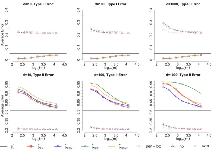
We then move on to evaluate the trend of type I and type II errors as the sample size increases in Figure 1. All the Neyman-Pearson based classifiers have type I error approaching α from below as sample size increases and they have similar type I errors at each sample size. However, nb, pen-log and svm all lead to a type I error larger than α.
By enlarging the second row of Figure 1, one would observe the differences in type II errors among PN2, PSN2, NN2, NSN2. In the case of d = 10 when all features are signals, PN2 performs the best throughout all sample sizes since it assumes the correct model without the unnecessary screening substep. When sample size is small, PSN2 outperforms NN2, but NN2 gradually catches up on larger samples. In the case of d = 100, screening helps PSN2 to take the lead at low sample sizes. The advantage of screening fades off as the sample size increases. In the case of d = 1000, PSN2 dominates all other three classifiers throughout the sample size range we investigate.
Overall, the advantage of PSN2 over NSN2, and PN2 over NN2 are uniform across all dimensions and sample sizes. This is consistent with the intuition that when the data are from a two-class Gaussian model, the parametric methods lead to more efficient estimators than nonparametric counterparts.
3.1.2 Example 2: normal vs. mixture normal
Normality assumption is violated in the second example. Assume p ∼ 0.5N(a,Σ) +
0.5N(−a,Σ) and q ∼ N(0d, Id), wherea= (√3101010,00d−10)0, Σ =
10−1I10 0 0 Id−10
. At
significance levelα= 0.05,the oracle type I/II risks areR0(φα∗) = 0.05 andR1(φ∗α) = 0.027 respectively.
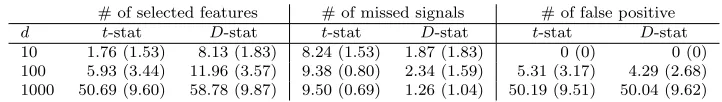
The performance of the screening substep of PSN2 and NSN2 is shown in Table 4. While both screening methods keep the false positive rates at around 1−Q, the parametric screening method (PSN2) with t-statistic misses almost all signals. This is not surprising sincet-statistics rank features by differences in means and the two groups have exactly the same marginal mean and variance across all dimensions.
Table 4: Average screening performance summarized over 1000 independent replications at sample sizesm=n= 400 andQ= 0.95 with standard errors in parentheses.
# of selected features # of missed signals # of false positive d t-stat D-stat t-stat D-stat t-stat D-stat 10 1.76 (1.53) 8.13 (1.83) 8.24 (1.53) 1.87 (1.83) 0 (0) 0 (0) 100 5.93 (3.44) 11.96 (3.57) 9.38 (0.80) 2.34 (1.59) 5.31 (3.17) 4.29 (2.68) 1000 50.69 (9.60) 58.78 (9.87) 9.50 (0.69) 1.26 (1.04) 50.19 (9.51) 50.04 (9.62)
Figure 2: Average error rates of ˆφ’s over 1000 independent replications for each combination of (d, m, n). Error rates are computed as the average of 1000 independent testing data points from each class in each replication, and then average over replications.
well on non-normal data. Their difference in type II error performances are similar as in Example 1.
From the two simulation examples, it is clear that the screening-based NSN2 and PSN2 exhibit advantages over their non-screening counterparts under high-dimensional settings. When the normality assumption is violated, and the sample sizes are reasonably large for efficient kernel estimates, NSN2 prevails over PSN2 . As a rule of thumb, for high-dimensional classification problems that emphasize type I error control, we recommend NSN2 if the sample size is relatively large and PSN2 otherwise.
3.2 Real data analysis
3.2.1 p53 mutants dataset
The p53 mutants dataset (Danziger et al., 2006) containsd= 5407 attributes extracted from biophysical experiments for 16772 mutant p53 proteins, among which 143 are determined as “active” and the rest as “inactive” via in vivo assays.
All 143 active samples and the first 1500 inactive samples are included in our analysis. We treat the active class as class 0 and aimed to control the error of missing an active under
α = 0.05. This dataset is split into a training set with 100 observations from the active class and 1000 observations from the inactive class, and a testing set with the remaining observations. PSN2 is used as the representative of our proposed methods, as the class 0 sample size is small for nonparametric methods. The average type I and type II errors over 1000 random splits are shown in Table 5. Compared with pen-log, nb and svm, PSN2 performs much better in controlling the type I error.
Table 5: Average errors over 1000 random splits with standard errors in parentheses. α= 0.05,δ1 = 0.05,Q= 0.95, andδ3 = 0.1.
PSN2 pen-log nb svm
type I .019 (.028) .162 (.060) .054 (.035) .275 (.189)
type II .461 (.291) .010 (.004) .384 (.427) .344 (.457)
3.2.2 Email spam dataset
Now, we consider an e-mail spam dataset available athttps://archive.ics.uci.edu/ml/ datasets/Spambase, which contains 4601 observations with 57 features, among which 2788 are class 0 (non-spam) and 1813 are class 1 (spam). We first standardize each feature and add 5000 synthetic features consisting of independentN(0,1) variables to make the problem more challenging. The augmented data has n= 4601 observations with d= 5057 features. This augmented dataset is split into a training set with 1000 observations from each class and a testing set with the remaining observations. We use NSN2 since the sample size is relatively large. The average type I and type II errors over 1000 random splits are shown in Table 6.
To evaluate the flexibility of NSN2 in terms of prioritized error control, we also report the performance when the priority is switched to control the type II error below α= 0.05. The results in Table 6 demonstrate that NSN2 is able to control either type I or type II error depending on the specific need of the practitioner.
4. Discussion
Table 6: Average errors over 1000 random splits with standard errors in parentheses. α= 0.05,δ1= 0.05,Q= 0.95, andδ3 = 0.05. The suffix after NSN2 indicates the type of error it targets to control underα.
NSN2-R0 NSN2-R1 pen-log nb svm type I .019 (.007) .488 (.078) .064 (.007) .423 (.024) .099 (.012)
type II .439 (.057) .020 (.009) .133 (.015) .058 (.010) .174 (.016)
It is also worthwhile to study the non-probabilistic approaches under high-dimensional NP paradigm. Methods of potential interest include theknearest neighbor (Weiss et al., 2010) and the centroid based classifiers (Tibshirani et al., 2002; Hall et al., 2010). However, the NP oracle inequalities are likely to be replaced by a new theoretical formulation for these methods.
A benefit of the present approach is that, for any given estimator ˆr, we have a uniform method to determine the proper threshold level in the plug-in classifiers. However, it would be interesting to develop new ways to estimate the threshold level Cα that is adaptive to the particular method used to approximate the density ratio r. Another future work is to study the theoretical properties of the permutation based choice of the threshold for the screening step.
Acknowledgements
The authors would like to thank the Editor and two anonymous referees for constructive comments. This research is partially supported by NSF CAREER grant DMS-1554804 (Feng), Lenfest Junior Faculty Development Grant from Columbia University (Feng), NSF grant DMS-1613338 (Tong), and NIH grant GM120507 (Tong).
Appendix A. Technical Lemmas and Proofs
Let Bin.cdfn, p(·) denote thecdfof Bin(n, p), and Beta.cdfa, b(·) denote thecdfof Beta(a, b).
The following lemma proves a duality between the beta and binomial distributions.
Lemma A.1 (Beta-binomial duality). For any p∈[0,1]and k∈ {1, . . . , n}, it holds that
1−Bin.cdfn, p(k−1) = Beta.cdfk, n+1−k(p).
Proof of Lemma A.1. Let U1, . . . , Un be n i.i.d. Uniform[0,1]. For any p ∈[0,1], let Np =
Pn
i=11I{Ui≤p} denote the number ofUi’s that are less or equal to p. Given IP(1I{Ui ≤p}= 1) = IP(Ui ≤p) = p , 1I{Ui ≤p} ∼ Bern(p) ∀i ,
we have Np ∼Bin(n, p), and therefore
On the other hand, let U(k) denote the k-th order statistic of {Ui}ni=1. It follows from the definition of order statistics that
{Np≥k} = {at leastk ofU1, . . . , Un are less or equal to p} =
U(k) ≤p . (A.2) Combining (A.1) with (A.2) yields
1−Bin.cdfn,p(k−1) = IP (Np≥k) = IP U(k)≤p
= Beta.cdfk, n+1−k(p) ,
where the last equality follows from U(k) ∼ Beta(k, n+ 1−k) (k = 1, . . . , n) as a direct implication of R´enyi’s representation. This completes the proof.
Lemma A.2. Let Z be a random variable from cdfF. We have
PF{F(Z)< δ} ≤ δ , PF {F(Z)> δ} ≥ 1−δ ∀δ∈[0,1]. (A.3)
For continuous F, the inequality becomes equality as
PF{F(Z)< δ} = δ , PF {F(Z)> δ} = 1−δ ∀δ∈[0,1]. (A.4)
.
Proof. Lett1 = min{t:F(t)≥δ}. Given the right continuity ofF, it can be easily proved by contradiction that i)F(t1−) =F(t1) =δ ifF is continuous at t1, and ii)F(t1−)< δ≤
F(t1) if F is discontinuous at t1. Thus,
PF{F(Z)< δ} = PF(Z < t1) = F(t1−) ≤ δ .
Likewise, let t2 = inf{t:F(t)> δ}. We have i) F(t2−) =F(t2) =δ ifF is continuous at
t2, and ii) F(t2−)< δ≤F(t2) if F is discontinuous att2. As a result,
PF{F(Z)> δ} = PF {Z ≥t2} = 1−PF{Z < t2} ≥ 1−δ . This completes the proof.
Lemma A.3. Let S ={Zi}ni=1 be a set n i.i.d. random variables from distribution F, and let Z(k) denote its k-th order statistic (k= 1, . . . , n). For any δ ∈(0,1), the probability of a new, independent realization Z from F to be greater than Z(k) satisfies
IPPF Z > Z(k)| S
> δ ≤ 1−Bin.cdfn,1−δ(k−1), (A.5) IP
PF Z > Z(k)| S
< δ ≥ 1−Bin.cdfn,δ(n−k) = Bin.cdfn,1−δ(k−1).(A.6)
The inequalities become equalities if F is continuous.
Proof of Lemma A.3. Rewrite the left-hand side of (A.5) as
IP
PF Z > Z(k) | S
> δ = IP
1−PF Z ≤Z(k)| S
> δ
= IP1−F(Z(k))> δ = IP
To bound the probability of{F(Z(k))<1−δ}, let N1−δ = Pni=11I{F(Zi)<1−δ} denote the
number ofF(Zi)’s that are less than 1−δ. It follows fromF(Z(1))≤F(Z(2))≤. . .≤F(Z(n)) that
F(Z(k))<1−δ =
F(Z(i))<1−δ , i= 1, . . . , k = {N1−δ≥k} , IP
F(Z(k))<1−δ = IP (N1−δ≥k) . (A.8) Letτ =PF {F(Z1)<1−δ}denote the success probability ofN1−δ as a binomial. It follows from (A.3) that τ ≤ 1−δ. Given Bin.cdfn,p(k−1) being decreasing in p for any fixed n and k, we have
IP (N1−δ ≥k) = 1−Bin.cdfn,τ(k−1) ≤1−Bin.cdfn,1−δ(k−1) (A.9) as a result of The equalities hold for continuous F. Connecting (A.7), (A.8), and (A.9) together yields
IPPF Z > Z(k) | S
> δ = IPF(Z(k))<1−δ = IP (N1−δ≥k)
≤ 1−Bin.cdfn,1−δ(k−1).
Likewise, let M1−δ = Pni=11I{F(Zi)>1−δ} be a binomial random variable with size n and
success rate τ0 = PF{F(Zi)>1−δ} ≥ δ that represents the number ofF(Zi)’s that are greater than 1−δ. The left-hand side of (A.6) can be rewritten as
IP
PF Z > Z(k)| S
< δ = IP
F(Z(k))>1−δ
= IP
F(Z(i))>1−δ , i=k, . . . , n = IP{M1−δ≥n+ 1−k} = 1−IP{M1−δ ≤n−k} = 1−Bin.cdfn,τ0(n−k)
≥ 1−Bin.cdfn, δ(n−k). (A.10)
This completes the proof.
Proof of Proposition 2.1. Letting Zi= ˆri,n=m3 in Lemma (A.3) yields IP{R0( ˆφk)> δ} ≤ 1−Bin.cdfm3,1−δ(k−1). This, together with Lemma A.1, completes the proof.
Lemma A.4. For random variable Z ∼Beta(a, b), and any >0,we have
IP{Z >(1 +)IEZ}<IP(|Z−IEZ|> IEZ)< b
−2
(a+b+ 1)a. (A.11)
Proof of Lemma A.4. By Chebyshev inequality,
IP(|Z−IEZ|> IEZ)≤ var(Z)
(IEZ)2 =
ab
(a+b)2(a+b+ 1)
a a+b
−2
= b
Proof of Proposition 2.2. Let B be a realization from Beta(k, m3+ 1−k). It follows from Proposition 2.1 that
IP{R0( ˆφk)> g(δ3, m3, k)} ≤ Beta.cdfk,m3+1−k{1−g(δ3, m3, k)}
= IP{B ≤1−g(δ3, m3, k)} = IP{1−B ≥g(δ3, m3, k)} for any k∈ {1,· · · , m3}and ˆr, with 1−B ∼Beta(m3+ 1−k, k). Letting a=m3+ 1−k,
b=k, and =k1/2{δ3(m3+ 2)(m3+ 1−k)}−1/2 in Lemma A.4 yields IP{R0( ˆφk)> g(δ3, m3, k)} ≤ δ3,
where
g(δ3, m3, k) = (1 +)
m3+ 1−k
m3+ 1
= m3+ 1−k
m3+ 1 +
s
k(m3+ 1−k)
δ3(m3+ 2)(m3+ 1)2
.
This completes the proof.
Proof of Proposition 2.3. By some basic algebra we have
Aα,δ3(m3)−(1−α) =
−1 + 2α+p1 + 4δ3(1−α)α(m3+ 2) 2{δ3(m3+ 2) + 1}
>0,
Aα,δ3(m3)−1 =
−1−2δ3(m3+ 2)α+
p
1 + 4δ3(1−α)α(m3+ 2) 2{δ3(m3+ 2) + 1}
<0,
and
g(δ3, m3, k) =
m3+ 1−k
m3+ 1 +
s
k(m3+ 1−k)
δ3(m3+ 2)(m3+ 1)2
≤α
⇔
k−(1−α)(m3+ 1)≥0,
{δ3(m3+ 2) + 1}
k m3+1
2
− {1 + 2δ3(m3+ 2)(1−α)}
k m3+1
+δ3(m3+ 2)(1−α)2≥0
⇔ k≥(m3+ 1) max{1−α, Aα,δ3(m3)}
⇔ k≥(m3+ 1)Aα,δ3(m3). Thus,
kmin(α, δ3, m3) =d(m3+ 1)Aα,δ3(m3)e
∈[(m3+ 1)Aα,δ3(m3),(m3+ 1)Aα,δ3(m3) + 1] . Since Aα,δ3(m3)→1−α, asm3 → ∞,it follows from sandwich rule that
lim m3→∞
kmin(α, δ3, m3)
m3
= lim m3→∞
We have kmin(α, δ3, m3)∈ K(α, δ3, m3) (⇔kmin(α, δ3, m3)≤m3) as long as (m3+ 1)Aα,δ3(m3) + 1 ≤ m3 ⇔ (1−α ≤) Aα,δ3(m3) ≤
m3−1
m3+ 1
. (A.12)
For any ∆∈(0, α), a sufficient condition for (A.12) is
m3−1
m3+ 1
≥1−∆, Aα,δ3(m3)≤1−∆, which can be further simplified as
m3≥ 2
∆−1, m3 ≥x ∗−
2,
where
x∗ = −2∆
2−α2+ 2α∆ + ∆ + (1−2α)∆ +α2 2(α−∆)2δ
3
= ∆(1−∆) (α−∆)2δ 3 is the positive root of the quadratic equation
(α−∆)2δ32x2+δ3 2∆2+α2−2α∆−∆
x−∆(1−∆) = 0.
Thus, a sufficient condition for (A.12) is
m3 ≥max
∆(1−∆) (α−∆)2δ
3
−2, 2
∆−1
.
Setting ∆ =α/2 yields
max
∆(1−∆) (α−∆)2 ·
1
δ3
−2, 2
∆−1
= max
2−α αδ3
−2,4 α −1
≤ 4
αδ3
.
Therefore, m3 ≥4/(αδ3) guarantees (A.12) andkmin(α, δ3, m3) ∈ K(α, δ3, m3). This com-pletes the proof.
Proof of Lemma 2.1. Introduce shorthand notation letA=Aα,δ3(m3) (defined in Proposi-tion 2.3) andα1 = (m3+1−kmin)/(m3+1) for simplicity of exposition. For anyB1, B2∈IR+, we have
{|R0( ˆφ)−α|> B1+B2} ⊂ {|R0( ˆφ)−α1|> B1} ∪ {|α1−α|> B2}, and thus
IP{|R0( ˆφ)−α|> B1+B2|rˆ}
≤ IP{|R0( ˆφ)−α1|> B1|rˆ}+ IP (|α1−α|> B2 |rˆ)
≤ kmin(m3+ 1−kmin)
(m3+ 2)(m3+ 1)2
where the last inequality follows from applying Lemma A.4 toR0( ˆφ) which follows Beta(m3+ 1−kmin, kmin) for m3 ≥ 4/(αδ3) and continuous Frˆ due to Lemma A.3. It follows from Proposition 2.3 that
|α−α1| ≤ A−(1−α) + 1
m3+ 1
. (A.14)
LettingB1 =
q
kmin(m3+1−kmin)
(m3+2)(m3+1)2δ4 and B2=A−(1−α) + 1
m3+1 in (A.13) yields
IP{|R0( ˆφ)−α|> ξα,δ3,m3(δ4)|rˆ}
≤ δ4+ 1I{|α1−α|> A−(1−α) + 1
m3+ 1
}
= δ4
for any arbitrary ˆr. This, together with the independence between S0
3 and ˆr (as a function of (S0
1,S11,S20,S21)) yields
IP{|R0( ˆφ)−α|> ξα,δ3,m3(δ4)} ≤ δ4.
To establish an upper bound for ξα,δ3,m3(δ4), note that
ξα,δ3,m3(δ4) =
s
kmin(m3+ 1−kmin) (m3+ 2)(m3+ 1)2δ4
+−1 + 2α+
p
1 + 4δ3(1−α)α(m3+ 2) 2{δ3(m3+ 2) + 1}
+ 1
m3+ 1
≤ s
(m3+ 1)2/4 (m3+ 2)(m3+ 1)2δ4
+ 1
2{δ3(m3+ 2) + 1} +
p
1 +δ3(m3+ 2) 2{δ3(m3+ 2) + 1}
+ 1
m3+ 1
< 1
2√m3δ4
+ 1
2m3δ3
+ 1
2√m3δ3 + 1
m3
.
When m3 ≥max(δ3−2, δ −2
4 ), we have
ξα,δ3,m3(δ4)< 1
2m1/43
+ 1
2m1/23
+ 1
2m1/43
+ 1
m3
= 1
m1/43 1 +
1
2m1/43 +
1
m3/43
!
< 5/2 m1/43 =
2 5m
1/4 3
−1
.
Proof of Proposition 2.4. Let G∗ ={r < Cα} and Gb ={r <ˆ Cbα}, the excess type II error
can be decomposed as:
P1(Gb)−P1(G∗)
=
Z
b G
dP1−
Z
G∗
dP1 =
Z
b G
p qdP0−
Z
G∗
p q dP0
=
Z
b G
(r−Cα)dP0+CαP0(Gb)− Z
G∗
(r−Cα)dP0−CαP0(G∗) =
Z
b G\G∗
(r−Cα)dP0−
Z
G∗\Gb
(r−Cα)dP0+Cα{P0(Gb)−P0(G∗)}
=
Z
b G\G∗
|r−Cα|dP0+
Z
G∗\Gb
|r−Cα|dP0+Cα{R0(φ∗)−R0( ˆφ)}. (A.15)
It follows from Lemma 2.1 that whenm3 ≥max{αδ43, δ3−2, δ4−2,(25M1δ∗ γ −
)−4},
ξα,δ3,m3(δ4)≤ 5 2m
−1/4
3 ≤M1(δ∗) γ −
,
ξα,δ3,m3(δ4)
M1
1/γ− ≤δ∗.
Introduce shorthand notations ∆R0 = |R0(φ∗)−R0( ˆφ)|, E0 = {∆R0 < ξα,δ3,m3(δ4)}, and
T =krˆ−rk∞. On the event E0,
∆R0
M1
1/γ− ≤
ξα,δ3,m3(δ4)
M1
1/γ− ≤ δ∗.
By the detection condition, we have
∆R0 ≤ P0{Cα< r(X)< Cα+ (∆R0/M1) 1/γ−
}.
Note that
P0{r(X)≥Cα+ (∆R0/M1) 1/γ−
}= R0(φ∗)−P0{Cα < r(X)< Cα+ (∆R0/M1) 1/γ−
}
≤ R0(φ∗)−∆R0
≤ R0( ˆφ) = P0{rˆ(X)>Cbα}
≤ P0{r(X) +T ≥Cbα} = P0{r(X)≥Cbα−T}.
Thus, we have Cbα≤Cα+ (∆R0/M1)
1/γ−
+T, and
b
G\G∗= {r≥Cα,r <ˆ Cbα}={r≥Cα,r < Cˆ α+ (∆R0/M1)
1/γ−
+T} ∩ {r <ˆ Cbα}
={Cα+ (∆R0/M1) 1/γ−
+ 2T ≥r ≥Cα,r < Cˆ α+ (∆R0/M1) 1/γ−
+T} ∩ {ˆr <Cbα}
⊂ {Cα+ (∆R0/M1) 1/γ−
+ 2T ≥r ≥Cα}.
Therefore, the margin assumption implies
P0(Gb\G∗) ≤ P0{Cα+ (∆R0/M1) 1/γ−
+ 2T ≥r≥Cα}
≤ M0{(∆R0/M1) 1/γ−
Hence on the event E0,
Z
b G\G∗
|r−Cα|dP0 ≤ {(∆R0/M1) 1/γ−
+ 2T}P0(Gb\G∗) ≤ M0{(∆R0/M1)
1/γ−
+ 2T}1+¯γ.
We will bound R
G∗\Gb|r−Cα|dP0 on the eventE1 ={R0( ˆφ)≤α}. Note that
P0(r≥Cα) =α≥R0( ˆφ) =P0(ˆr ≥Cbα)≥P0(r≥Cbα+krˆ−rk∞) =P0(r≥Cbα+T).
The above chain implies thatCbα≥Cα−T. Therefore,
G∗\Gb={r < Cα,rˆ≥Cbα}
={r < Cα, r≥r−ˆr+Cbα}
⊂ {r < Cα, r≥Cbα−T} ⊂ {Cα−2T ≤r ≤Cα}.
Hence on the event E1,
Z
G∗\ b G
|r−Cα|dP0≤2T·P0(Cα−2T ≤r≤Cα)≤M0(2T)1+¯γ,
where the last inequality follows from the margin assumption. Then it follows from (A.15) that on the event E0∩ E1,
R1( ˆφ)−R1(φ∗) ≤ M0
" |
∆R|
M1
1/γ−
+ 2T
#1+¯γ
+M0(2T)1+¯γ+Cα|R0( ˆφ)−R0(φ∗)|
≤ 2M0
"
ξα,δ3,m3(δ4)
M1
1/γ−
+ 2T
#1+¯γ
+Cα·ξα,δ3,m3(δ4).
From Lemma 2.1, we know that the event E0 occurs with probability at least 1−δ4. By Proposition 2.2 and Proposition 2.3 we know eventE1occurs with probability at least 1−δ3, soE0∩ E1 occurs with probability at least 1−δ3−δ4. This completes the proof.
Proof of Proposition 2.5. Define event
Eδ1 = d
\
j=1
{kFˆj1−Fj1k∞< δ11} ∩ {kFˆj0−Fj0k∞< δ10},
whereδ11 =
q
log(4d/δ1) 2n1 and δ
0 1 =
q
log(4d/δ1)
2m1 .On the eventEδ1, for anyj∈ A,
kFˆj0−Fˆj1k∞≥ kFj0−Fj1k∞− kFj0−Fˆj0k∞− kFj1−Fˆj1k∞
≥D− kFj0−Fˆj0k∞− kFj1−Fˆj1k∞
For anyj6∈ A,
kFˆj0−Fˆj1k∞≤ kFj0−Fˆj0k∞+kFj0−Fj1k∞+kFj1−Fˆj1k∞ =kFj0−Fˆj0k∞+kFj1−Fˆj1k∞
< δ01+δ11.
Since n1 ≥ 8D−2log(4d/δ1) and m1 ≥8D−2log(4d/δ1), δ01 +δ11 ≤ D−δ10−δ11. As a result, on the eventEδ1,any τ ∈
δ10+δ11, D−δ01−δ11
would lead toAbτ =A. Therefore,
IP(Abτ =A)≥ IP(Eδ1)
≥ 1−
d
X
j=1
n
IP(kFˆj1−Fj1k∞≥δ11) + IP(kFˆj0−Fj0k∞≥δ10)
o
≥ 1−δ1,
where the last inequality follows from applying Lemma A.5 to Fj0 and Fj1 forj= 1,· · · , d. This completes the proof.
Proof of Proposition 2.6. Define event
E= \
j∈A
{klog ˆpj−logpjk∞< Bj1} ∩ {klog ˆqj−logqjk∞< Bj0},
where
Bj1 =
Cj1
q
log(2n2s/δ2) n2h1
µ−Cj1
q
log(2n2s/δ2) n2h1
, Bj0=
Cj0
q
log(2m2s/δ2) m2h0
µ−Cj0
q
log(2m2s/δ2) m2h0
.
Let B1 = supj∈ABj1 and B0 = supj∈ABj0, we have B ≥ s(B0 +B1). On the event
{Abτ =A} ∩ E,we have
log ˆrNS(x) = X j∈Ab
logpˆj(xj) ˆ
qj(xj)
= X
j∈A
log ˆpj(xj)−
X
j∈A
log ˆqj(xj).
Therefore,
klog ˆrSN−logrk∞ = k
X
j∈A
log ˆpj −
X
j∈A
log ˆqj −
X
j∈A
logpj+
X
j∈A
logqjk∞
≤ X
j∈A
(klog ˆpj−logpjk∞+klog ˆqj−logqjk∞)
≤ X
j∈A
(B1+B0) ≤ B .
On the event{Abτ =A} ∩ E, it follows from Lagrange’s mean value theorem that for anyx,
there exists somewx between log ˆrSN(x) and logr(x) such that
|rˆSN(x)−r(x)| = |elog ˆrNS(x)−elogr(x)| = ewx|log ˆrS
N(x)−logr(x)|
where the last inequality follows from the fact that
wx≤max(logr(x),log ˆrNS(x))≤max(klogrk∞,klog ˆrNSk∞)≤ klogrk∞+B . Thus,krˆSN−rk∞≤T , and we have
IP krˆSN−rk∞≤T ≥ IP({Abτ =A} ∩ E) ≥ IP(Abτ =A) + IP(E)−1
= IP(Abτ =A)−IP(Ec). (A.16)
By Proposition 2.5, we have
IP(Abτ =A) ≥ 1−δ1. (A.17)
Also, it follows from Lemma A.6 that
IP klog ˆpj−logpjk∞> Bj1
∨IP klog ˆqj−logqjk∞> Bj0
≤ δ2/(2s). Therefore,
IP(Ec) ≤ (2s)δ2/(2s) = δ2. (A.18) Plugging (A.17) and (A.18) back to (A.16) yields (2.16). Moreover, because s≤n2∧m2, it follows from Lemma A.6 that there exists some ¯C2>0, such that
B ≤ C¯2s
(
logn2
n2
2ββ+1
+
logm2
m2
2ββ+1)
.
Moreover, sinces≤(n2∧m2)
β
2(β+1), the above bound implies thatB is bounded from above by some absolute constant. Also note that krk∞ is bounded from above, so there exists an absolute constant C2 >0, such that
T =BeBkrk∞≤C2s
(
logn2
n2
2ββ+1
+
logm2
m2
2ββ+1)
.
This completes the proof.
Proof of Theorem 2.1. Combining Propositions 2.2, 2.3, 2.4 and 2.6,
IPR0( ˆφNSN2)≤α, R1( ˆφNSN2)≤R1(φ∗) +W
≥1−δ1−δ2−δ3−δ4, where
W = 2M0
"
2 5m
1/4 3 M1
−1/γ−
+ 2C2s
(
logn2
n2
2ββ+1
+
logm2
m2
2ββ+1)#1+¯γ
+ Cα
2 5m
1/4 3
−1
.
Lemma A.5(Dvoretzky-Kiefer-Wolfowitz inequality(Dvoretzky et al., 1956)). Let X1,X2,
· · ·,Xnbe real-valued i.i.d. random variables withcdfF(·), and letFˆn(x) =n−1Pni=11I(Xi≤
x). For anyt >0, it holds that
IP(kFˆn−Fk∞≥t) ≤ 2e−2nt 2
.
Or, for any givenδ ∈(0,1),
IP(kFˆn−Fk∞≥
r
log(2/δ)
2n ) ≤ δ . (A.19)
Lemma A.6. Given a density function p∈ PΣ(β, L,[−1,1]), construct its kernel estimate ˆ
p(x) = (nh)−1Pn
i=1K
Xi−x
h
from i.i.d. sample {Xi}ni=1, where the kernel K is β-valid
and L0-Lipschitz, and the bandwidth h = (logn/n)2β1+1. For any δ ∈(0,1), as long as the
sample size n is such that
q
log(n/δ)
nh < min(1, µ/C), where C =
√
48c1 + 32c2 + 2Lc3 +
L0 +L + ˜CP
1≤|l|≤bβcl!1, in which c1 = kpk∞kKk 2
2, c2 = kKk∞+kpk∞+R |K||t|βdt,
c3 =
R
|K||t|βdt, and C˜ is such that C˜ ≥ sup
1≤|l|≤bβcsupx∈[−1,1]|p(l)(x)|, and µ(>0) is a lower bound of p, we have
IP (klog ˆp−logpk∞≥U) ≤ δ , (A.20)
where U = C q
log(n/δ)
nh
µ−C q
log(n/δ)
nh
. When n≥1/δ, we have U ≤C1(logn/n)
β
2β+1 for some absolute
constant C1.
Proof. LetE1 ={kpˆ−pk∞≤C
q
log(n/δ)
nh }. On the eventE1, since
q
log(n/δ)
nh <min(1, µ/C), we have
min(p(x0),pˆ(x0))≥min(p(x0), p(x0)− kpˆ−pk∞)≥µ− kpˆ−pk∞>0.
It then follows from Lagrange’s mean value theorem that for any fixedx0,there exists some
wx0 between ˆp(x0) andp(x0),
|log ˆp(x0)−logp(x0)|= wx−10 |pˆ(x0)−p(x0)|
≤ [min{pˆ(x0), p(x0)}]−1|pˆ(x0)−p(x0)| ≤
kpˆ−pk∞
µ− kpˆ−pk∞
.
As a result, it holds on eventE1 that
klog ˆp−logpk∞ ≤
C
q
log(n/δ) nh
µ−C
q
log(n/δ) nh
= U ,
and
IP(klog ˆp−logpk∞≤U)≥IP(kpˆ−pk∞≤C
r
log(n/δ)
nh )≥1−δ ,
where the last inequality follows from Lemma A.1 in Tong (2013) (the special case of
d = 1). Finally when n ≥ 1/δ, we have U = C q
log(n/δ)
nh
µ−C q
log(n/δ)
nh
≤ C1(logn/n)
β
2β+1 for some