Input Output Kernel Regression: Supervised and Semi-Supervised Structured Output Prediction with Operator-Valued Kernels

Input Output Kernel Regression: Supervised and

Semi-Supervised Structured Output Prediction with

Operator-Valued Kernels

C´eline Brouard [email protected]

Helsinki Institute for Information Technology HIIT Department of Computer Science, Aalto University 02150 Espoo, Finland

IBISC, Universit´e d’ ´Evry Val d’Essonne 91037 ´Evry cedex, France

Marie Szafranski [email protected]

ENSIIE & LaMME, Universit´e d’ ´Evry Val d’Essonne, CNRS, INRA 91037 ´Evry cedex, France

IBISC, Universit´e d’ ´Evry Val d’Essonne 91037 ´Evry cedex, France

Florence d’Alch´e-Buc [email protected]

LTCI, CNRS, T´el´ecom ParisTech Universit´e Paris-Saclay

46, rue Barrault 75013 Paris, France IBISC, Universit´e d’ ´Evry Val d’Essonne 91037 ´Evry cedex, France

Editor:Koji Tsuda

Abstract

In this paper, we introduce a novel approach, called Input Output Kernel Regression (IOKR), for learning mappings between structured inputs and structured outputs. The approach belongs to the family of Output Kernel Regression methods devoted to regres-sion in feature space endowed with some output kernel. In order to take into account structure in input data and benefit from kernels in the input space as well, we use the Re-producing Kernel Hilbert Space theory for vector-valued functions. We first recall the ridge solution for supervised learning and then study the regularized hinge loss-based solution used in Maximum Margin Regression. Both models are also developed in the context of semi-supervised setting. In addition we derive an extension of Generalized Cross Validation for model selection in the case of the least-square model. Finally we show the versatility of the IOKR framework on two different problems: link prediction seen as a structured output problem and multi-task regression seen as a multiple and interdependent output problem. Eventually, we present a set of detailed numerical results that shows the relevance of the method on these two tasks.

1. Introduction

Many real world applications involve objects with an explicit or implicit discrete structure. Texts, images and videos in document processing and retrieval as well as genes and proteins in computational biology are all examples of implicit structured data that we may want to use as inputs or outputs in a prediction system. Besides these structured objects, structured output prediction can also concern multiple outputs linked by some relationship that is rele-vant to take into account. Surprisingly, although a lot of attention has been paid to learning from structured inputs for now two decades, this problem, often referred asstructured output learning, has emerged relatively recently as a field of interest in statistical learning. In the literature, structured output prediction has been addressed from two main angles. A first angle consists indiscriminative learning algorithmsthat provide predictions by maximizing a scoring function over the output space. Conditional Random Fields (Lafferty et al., 2001) and their extension to kernels (Lafferty et al., 2004) were first proposed for discriminative modeling of graph-structured data and sequence labeling. Other discriminative learning al-gorithms based on maximum margin such as structured SVM (Tsochantaridis et al., 2004,

2005), Maximum Margin Markov Networks (M3N) (Taskar et al., 2004) or Maximum

Mar-gin Regression (Szedmak et al., 2005) have then be developed and thoroughly studied. A common approach to those methods consists in defining a linear scoring function based on the image of an input-output pair by a joint feature map. Both methods, either based on Conditional Random Fields or maximum-margin techniques, are costly to train and gener-ally assume that the output set_Y is discrete. Keeping the idea of a joint feature map over inputs and outputs, a generative method called Joint Kernel Support Estimation has been recently proposed (Lampert and Blaschko, 2009). In this approach, a one-class SVM is used to learn the support of the joint-probability densityp(x, y). More recently, another angle to

structured output prediction, that we calledOutput Kernel Regression(OKR), has emerged

In this work, we therefore propose to extend the methodology of Output Kernel Re-gression to another large family of nonparametric reRe-gression tools that allows to tackle structured data in the input space as well as in the output space. Moreover we will show that this new family of tools is useful in a semi-supervised context. Called Input Output Kernel Regression, this novel family for structured output prediction from structured inputs relies on Reproducing Kernel Hilbert Spaces (RKHS) for vector-valued functions with the following specification: the output vector belongs to some output feature space associated to a chosen output kernel, as introduced in the works of Brouard et al. (2011) and Brouard (2013). Let us recall that in the case of scalar-valued functions, the RKHS theory offers a flexible framework for penalized regression as witnessed by the abundant literature on the subject (Wahba, 1990; Pearce and Wand, 2006). A penalized regression problem is seen as a minimization problem in a functional space built on an input scalar-valued ker-nel. Depending the nature of the prediction problem, appropriate penalties can be defined and representer theorem can be proven, facilitating the minimization problem to be further solved. In the RKHS theory, regularization constraint on the geometry of the probability distribution of labeled and unlabeled data can also be added to perform semi-supervised regression (Belkin et al., 2006). When functions are vector-valued, the adequate RKHS the-ory makes use of operator-valued kernels (Pedrick, 1957; Senkene and Tempel’man, 1973; Micchelli and Pontil, 2005). Operator-valued kernels have already been proposed to solve problems of multi-task regression (Evgeniou et al., 2005; Baldassarre et al., 2012), struc-tured classification (Dinuzzo et al., 2011), vector autoregression (Lim et al., 2013) as well as functional regression (Kadri et al., 2010). The originality of this work is to consider that the output space is a feature space associated to a chosen output kernel. This new approach not only enhances setting of pattern recognition tasks by requiring to pay attention on both input and output sets but also opens new perspectives in machine learning. It encompasses in a unique framework kernel-based regression tools devoted to structured inputs as well as structured outputs.

1.1 Related Works

In Brouard et al. (2011), the vector-valued RKHS theory was used to address the output kernel regression problem in the semi-supervised setting. This approach was applied to the link prediction problem. By working in the framework of RKHS theory for vector-valued functions, we extended the manifold regularization framework introduced by Belkin et al. (2006) to functions with values in a Hilbert space. We have also shown that the first step of KDE (Cortes et al., 2005) is a special case of IOKR using a particular operator-valued kernel.

In parallel of Brouard et al. (2011), Minh and Sindhwani (2011) generalized the manifold regularization framework proposed by Belkin et al. (2006) for semi-supervised learning to vector-valued functions.

1.2 Contributions

We introduce Input Output Kernel Regression (IOKR), a novel class of penalized regression problems based on the definition of an output scalar-valued kernel and an input operator-valued kernel. This article is an extended version of Brouard et al. (2011), that addresses more generally the problem of structured output prediction. In this work, we present several novel contributions regarding the RKHS theory for functions with values in a Hilbert space. We present the representer theorem for vector-valued functions in the semi-supervised set-ting. Based on this representer theorem, we study two particular models obtained using

two different loss functions: theIOKR-ridgemodel introduced in Brouard et al. (2011) and

a new model called IOKR-margin. This model extends the Maximum Margin Regression

(MMR) framework introduced by Szedmak et al. (2005) to operator-valued kernels and to the semi-supervised setting. In this paper, we also put the reformulation of Kernel Depen-dency Estimation proposed by Cortes et al. (2005) into perspective in the Output Kernel Regression framework. We present the solutions corresponding to decomposable kernels. In the case of the least-squared loss function, we describe a new tool for model selection, which was first introduced in Brouard (2013). The selection of the hyperparameters is done by estimating the averaged error obtained with leave-one-out cross-validation as a closed-form solution. We show the versatility of the IOKR framework on two different problems: link prediction and multi-task regression. Finally, we present numerical results obtained with IOKR on these two tasks.

1.3 Organization of the Paper

This paper is organized as follows. In Section 2, we introduce the Input Output Kernel Regression approach and show how it can be used to solve structured output prediction problems. In Section 3 we describe the RKHS theory devoted to vector-valued function and present our contributions to this theory in the supervised and semi-supervised settings. We also present in this section models based on decomposable operator-valued kernels. We then show in Section 4 that, in the case of the least-squares loss function, the leave-one-out criterion can be estimated by a closed-form solution. In Section 5, we describe how Input Output Kernel Regression (IOKR) can be used to solve two structured prediction problems, which are link prediction and multi-task learning. In Section 6, we present the results obtained with IOKR on these two problems.

The notations used in this paper are summarized in Table 1.

2. From Output Kernel Regression to Input Output Kernel Regression

We consider the general regression task consisting in learning a mapping between an input

set _X and an output set _Y. We assume that both _X and _Y are sample spaces and that

Sn={(xi, yi), i= 1...n} is an i.i.d. sample drawn from the joint probability lawP defined

Meaning Symbol

number of labeled examples `

number of unlabeled examples n

input set _X

set of labeled examples X`

union of the labeled and unlabeled sets _X`+n

output set _Y

input scalar kernel κx:X × X →R

output scalar kernel κy :Y × Y →R

input feature space _Fx

output feature space Fy

input feature map ϕx :X → Fx

output feature map ϕy :Y → Fy

set of bounded operators from an Hilbert spaceF to itself B(F)

set of bounded operators from_F to an Hilbert space_{G B}(_F,_G)

operator-valued kernel _Kx:X × X → B(Fy)

reproducing kernel Hilbert space ofKx H,HKx

canonical feature map of_Kx φx :X → B(Fy,H)

gram matrix of_Kx on X` and X`+n KX`,KX`+n

gram matrix ofκx on X` and X`+n KX`, KX`+n

gram matrix ofκy onY` KY`

graph Laplacian L

matrix vectorization vec

Kronecker product ⊗

Hadamard product (element-wise product) _◦

Table 1: Notations used in this paper

graphs, nodes in a graph, or simply vectors of interdependent variables. It is realistic

to assume that one can build a similarity κy : Y × Y → R between the elements of the

output set _Y, such that κy takes into account the inherent structure of the elements of Y

and has the properties of a positive definite kernel. Then, due to the Moore-Aronszajn theorem (Aronszajn, 1950), there exists a Hilbert space Fy, called a feature space, and a

corresponding functionϕy :Y → Fy, called afeature mapsuch that:

∀(y, y0)_{∈ Y × Y}, κy(y, y0) =hϕy(y), ϕy(y0)iFy.

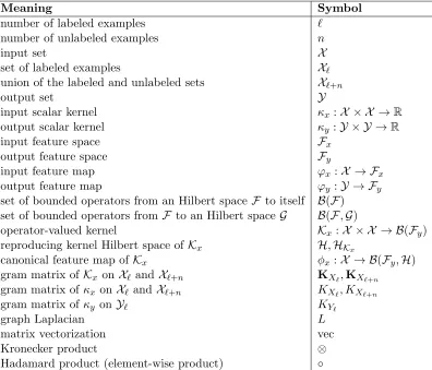
The regression problem betweenX andY can be decomposed into two tasks (see Figure 1):

• the first task is to learn a functionh from the setX to the Hilbert spaceFy

• the second one is to define or learn a function f from _Fy toY to provide an output

in the set Y.

We call the first task, Output Kernel Regression (OKR), referring to previous works

Fy

f

h

X

Y

ϕ

_y

Figure 1: Schema of the Output Kernel Regression approach.

pre-image problem. In this paper, we develop a general theoretical and practical framework for the OKR task, allowing to deal with structured inputs as well as structured outputs. To illustrate our approach, we have chosen two structured output learning tasks which do not

require to solve a pre-image problem. One is multi-task regressionfor which the dimension

of the output feature space is finite, and the other one islink predictionfor which prediction

in the original set _Y is not required. However, the approach we propose can be combined

with pre-image solvers now available on the shelves. The interested reader may want to refer to Honeine and Richard (2011) or Kadri et al. (2013) to benefit from existing pre-image algorithms to solve structured output learning tasks.

In this work, we propose to build a family of models and learning algorithms devoted to Output Kernel Regression that present two additional properties compared to OK3-based methods: namely, models are able to take into account structure in input data and can be learned within the framework of penalized regression, enjoying various penalties including smoothness penalties for semi-supervised learning. To achieve this goal, we choose to use

kernels both in the input and output spaces. As the models have values in a feature

space and not inR, we turn to the vector-valued reproducing kernel Hilbert spaces theory

(Pedrick, 1957; Senkene and Tempel’man, 1973; Burbea and Masani, 1984) to provide a general framework for penalized regression of nonparametric vector-valued functions. In that theory, the values of kernels are operators on the output vectors which belong to some Hilbert space. Introduced in machine learning by the seminal work of Micchelli and Pontil (2005) to solve multi-task regression problems, operator-valued kernels (OVK) have then been studied under the angle of their universality (Caponnetto et al. (2008); Carmeli et al. (2010)) and developed in different contexts such as structured classification (Dinuzzo et al., 2011), functional regression (Kadri et al., 2010), link prediction (Brouard et al., 2011) or semi-supervised learning (Minh and Sindhwani, 2011; Brouard et al., 2011). With operator-valued kernels, models of the following form can be constructed:

∀x∈ X, h(x) =

n

X

i=1

Kx(x, xi)ci, ci∈ Fy, xi∈ X, (1)

extending nicely the usual kernel-based models devoted to real-valued functions.

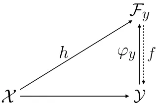
In the case of IOKR, the output Hilbert space _Fy is defined as a feature space related

to a given output kernel. Note that there exists different pairs (feature space, feature

Fy

g

f

h

X

Y

Fy

g

f

h

X

Y

Fx

φ

x

ϕ

_x

ϕ

_y

ϕ

y

B

(

_F

_y

,

_H

)

Figure 2: Diagrams describing Kernel Dependency Estimation (KDE) on the left and Input Output Kernel Regression (IOKR) on the right.

κy(y, y0) = (yTy0 +c)p: we can choose the finite feature space defined by the different

monomes of the coordinates of a vector y or we can choose the RKHS associated with

the polynomial kernel. This choice will open doors to different output feature spaces Fy,

leading to different definitions of the input operator-valued kernel _Kx and thus to different

learning problems. Omitting the choice of the feature map associated to _Fy, we therefore

need to define a triplet (κy,Fy,Kx) as a pre-requisite to solve the structured output learning

task. By explicitly requiring to define an output kernel we emphasize the fact that an input operator-valued kernel cannot be defined without calling into question the output space,

Fy, and therefore, the output kernelκy. We will show in Section 6 that the same structured

output prediction problem can be solved in different ways using different values for the triplet (κy,Fy,Kx).

Interestingly, IOKR generalizes Kernel Dependency Estimation (KDE), a problem that was introduced in Weston et al. (2003) and was reformulated in a more general way by

Cortes et al. (2005). If we call _Fx a feature space associated to a scalar input kernel

κx :X × X →R and ϕx :X → Fx a corresponding feature map, KDE uses Kernel Ridge

regression to learn a functionh from _X to_Fy by building a function g fromFx toFy and

composing it with the feature mapϕx (see Figure 2). The functionh is modeled as a linear

function: h(x) =W ϕx(x), where W is a linear operator from Fx toFy. The second phase

consists in computing the pre-image of the obtained prediction.

In the case of IOKR, we build models of the general form introduced in Equation (1).

Denoting φx the canonical feature map associated to the OVK Kx, which is defined as:

φx(x) = Kx(·, x), we can draw the chart depicted in Figure 2 on the right. The function

φx maps inputs fromX to B(Fy,H). Indeed the value φx(x)y =Kx(·, x)y is a function of

the RKHS_H for ally in _Fy. The model h is seen as the composition of a function g from

B(Fy,H) to the output feature spaceFy with the input feature map φx.

We can therefore see on Figure 2 how IOKR extends KDE. In Brouard et al. (2011), we have shown that we retrieve the model used in KDE when considering the following operator-valued kernel:

whereI is the identity operator from_FytoFy. Unlike KDE, that learns independently each

component of the vectors ϕy(y), IOKR takes into account the structure existing between

these components.

The next section is devoted to the RKHS theory for vector-valued functions and to our contributions to this theory in the supervised and semi-supervised settings.

3. Operator-Valued Kernel Regression

In the following, we briefly recall the main elements of the RKHS theory devoted to vector-valued functions (Senkene and Tempel’man, 1973; Micchelli and Pontil, 2005) and then present our contributions to this theory.

Let _X be a set and_Fy a Hilbert space. In this section, no assumption is needed about

the existence of an output kernelκy. We note ˜ythe vectors inFy. Given two Hilbert spaces

F and G, we note B(F,G) the set of bounded operators from F toG and B(F) the set of bounded operators from_F to itself. Given an operatorA,A∗ denotes the adjoint ofA.

Definition 1 An operator-valued kernel on X × X is a functionKx:X × X → B(Fy) that

verifies the two following conditions:

• ∀(x, x0)_{∈ X × X}, _Kx(x, x0) =Kx(x0, x)∗,

• ∀m_∈N, ∀Sm ={(xi,y˜i)}mi=1⊆ X × Fy, Pmi,j=1hy˜i,Kx(xi, xj)˜yjiFy ≥0.

The following theorem shows that given any operator-valued kernel, it is possible to build a reproducing kernel Hilbert space associated to this kernel.

Theorem 2 (Senkene and Tempel’man (1973); Micchelli and Pontil (2005)) Given an operator-valued kernel _Kx :X × X → B(Fy), there is a unique Hilbert space HKx

of functions h:_{X → F}y which satisfies the following reproducing property:

∀h_{∈ H}Kx,∀x∈ X, h(x) =Kx(x,·)h,

where _Kx(x,·) is an operator in B(HKx,Fy).

As a consequence, ∀x∈ X,∀y˜ ∈ Fy,∀h∈ HKx, hKx(·, x)˜y, hiHKx =hy˜, h(x)iFy.

The Hilbert space _HKx is called the reproducing kernel Hilbert space associated to the

kernel _Kx. This RKHS can be built by taking the closure of span{Kx(·, x)α|x ∈ X,α ∈

Fy}. The scalar product on HKx between two functions f =

Pn

i=1Kx(·, xi)αi and g =

Pm

j=1Kx(·, tj)βj, xi, tj ∈ X,αi,βj ∈ Fy,is defined as: hf, g_iHKx =

n

X

i=1

m

X

j=1

hαi,Kx(xi, tj)βjiFy.

The corresponding norm _{k · k}HKx is defined by kf k

2

HKx=hf, fiHKx. For sake of simplicity

we replace the notation_HKx by Hin the rest of the paper.

3.1 Regularization in Vector-Valued RKHS

Based on the RKHS theory for vector-valued functions, Micchelli and Pontil (2005) have proved a representer theorem for convex loss functions in the supervised case.

We noteS`={(xi,y˜i)}`i=1⊆ X × Fy the set of labeled examples and Hthe RKHS with

reproducing kernel _Kx :X × X → B(Fy).

Theorem 3 (Micchelli and Pontil (2005)) Let_L be a convex loss function, andλ1 >0 a regularization parameter. The minimizer of the following optimization problem:

argmin

h∈H J

(h) =

`

X

i=1

L(h(xi),y˜i) +λ1khk2H,

admits an expansion:

ˆ h(_·) =

`

X

j=1

Kx(·, xj)cj ,

where the coefficients cj, j= 1,· · · , `are vectors in the Hilbert space Fy.

In the following, we plug the expansion form of the minimizer into the optimization prob-lem and consider the probprob-lem of finding the coefficients cj for two different loss functions:

the least-squares loss and the hinge loss.

3.1.1 Penalized Least Squares

Considering the least-squares loss function for regularization of vector-valued functions, the minimization problem becomes:

argmin

h∈H J

(h) =

`

X

i=1

kh(xi)−y˜ik2Fy+λ1khk

2

H. (3)

Theorem 4 (Micchelli and Pontil (2005)) Letcj ∈ Fy, j = 1,· · ·, `, be the coefficients

of the expansion admitted by he minimizer ˆh of the optimization problem in Equation (3). The vectorscj ∈ Fy satisfy the equations:

`

X

i=1

(_Kx(xj, xi) +λ1δij)ci = ˜yj ,

where δ is the Kronecker symbol: δii= 1 and ∀j6=i, δij = 0.

Let c = (cj)`j=1 ∈ Fy` and ˜y = (˜yj)`j=1 ∈ Fy`. This system of equations can be

equiva-lently written (Micchelli and Pontil, 2005):

(SX`S

∗

X`+λ1I)c= ˜y,

where I denotes the identity operator from _Fy` to <sub>Fy</sub>` and SX` :H → F

`

y is the sampling

operator defined for every h _{∈ H} by: SX`h = (h(xi))

`

i=1. The expression of its adjoint S_X∗

` :F

`

y → Hof SX` for every c∈ F

`

y is given by: SX∗`c=

P`

i=1Kx(·, xi)ci. Therefore the

solution of the optimization problem in Equation (3) writes as:

hridge(x) =Kx(x,·)SX∗`(SX`S

∗

X`+λ1I)

3.1.2 Maximum Margin Regression

Szedmak et al. (2005) formulated a Support Vector Machine algorithm with vector output, called Maximum Margin Regression (MMR). The optimization problem of MMR in the supervised setting is the following:

argmin

h J

(h) =

`

X

i=1

max(0,1_{− h}y˜i, h(xi)iFy) +λ1khk

2

H. (4)

In Szedmak et al. (2005), the function h was modeled as: h(x) = W ϕx(x) +b, where

ϕx is a feature map associated to a scalar-valued kernel. In this subsection, we extend this

maximum margin based regression framework to the context of the vector-valued RKHS

theory by searching h in the RKHS_H associated to _Kx.

Similarly to SVM, the MMR problem (4) can be expressed according to a primal for-mulation that involves the optimization of h _{∈ H} and slack variablesξi ∈ R,i = 1, . . . , `, as well as its dual formulation which is expressed according to the Lagrangian parameters

α = [α1, . . . , α`]T ∈ R`. The latter leads to solve a quadratic program, for which efficient solvers exist. Both formulations are given below.

The primal form of the MMR optimization problem can be written as:

min

h∈H,{ξi∈R}`i=1

λ1khk2H+ `

X

i=1 ξi

s.t. _hy˜i, h(xi)iFy ≥1−ξi, i= 1, . . . , `

ξi≥0, i= 1, . . . , `.

The Lagrangian of the above problem is given by:

La(h,ξ,α,η) =λ1khk2H+ `

X

i=1 ξi−

`

X

i=1

αi(hKx(·, xi)˜yi, hiH−1 +ξi)− `

X

i=1 ηiξi,

withαi and ηi being Lagrange multipliers. By differentiating the Lagrangian with respect

toξi and h and setting the derivatives to zero, the dual form of the optimization problem

can be expressed as:

min

α∈R`

1 4λ1

`

X

i,j=1

αiαjhy˜i,Kx(xi, xj)˜yjiFy −

`

X

i=1 αi

s.t. 0_≤αi ≤1, i= 1, . . . , `

(5)

and the solution ˆh can be written as: ˆh(_·) = ₂1_λ 1

P`

j=1αjKx(·, xj)˜yj. Note that, similarly

to KDE, we retrieve the original MMR solution when using the following operator-valued kernel: _Kx(x, x0) =κx(x, x0)I.

3.2 Extension to Semi-Supervised Learning

In the case of real-valued functions, Belkin et al. (2006) have introduced a novel framework,

called manifold regularization. This approach is based on the assumption that the data

lie in a low-dimensional manifold. Belkin et al. (2006) have proved a representer theorem devoted to semi-supervised learning by adding a new regularization term which exploits the information of the geometric structure. This regularization term forces the target function

h to be smooth with respect to the underlying manifold. In general, the geometry of

this manifold is not known but it can be approximated by a graph. In this graph, nodes correspond to labeled and unlabeled data and edges reflect the local similarities between

data in the input space. For example, this graph can be built using k-nearest neighbors.

The representer theorem of Belkin et al. (2006) has been extended to the case of vector-valued functions in Brouard et al. (2011) and Minh and Sindhwani (2011). In the following, we present this theorem and derive the solutions for the least-squares loss function and maximum margin regression.

LetLbe a convex loss function. Given a set of`labeled examples{(xi,y˜i)}`i=1⊆ X ×Fy

and an additional set of n unlabeled examples _{xi}`i=+`n+1 ⊆ X, we consider the following optimization problem:

argmin

h∈H J

(h) =

`

X

i=1

L(h(xi),y˜i) +λ1khk2H+λ2

`+n

X

i,j=1

Wijkh(xi)−h(xj)k2Fy, (6)

where λ1, λ2 > 0 are two regularization hyperparameters and W is the adjacency matrix

of a graph built from labeled and unlabeled data. This matrix measures the similarity

between objects in the input space. We assume that the values of W are non-negative.

This optimization problem can be rewritten as:

argmin

h∈H J

(h) =

`

X

i=1

L(h(xi),y˜i) +λ1khk2H+ 2λ2

`+n

X

i,j=1

Lijhh(xi), h(xj)iFy,

where L is the graph Laplacian given by L = D−W, and D is the diagonal matrix of

general term Dii =

P`+n

j=1Wij. Instead of the graph Laplacian, other matrices, such as

iterated Laplacians or diffusion kernels (Kondor and Lafferty, 2002), can also be used.

Theorem 5 (Brouard et al. (2011); Minh and Sindhwani (2011)) The minimizer of the optimization problem in Equation (6) admits an expansion:

ˆ h(_·) =

`+n

X

j=1

Kx(·, xj)cj ,

for some vectors cj ∈ Fy, j = 1,· · · , `+n.

3.2.1 Semi-Supervised Penalized Least-Squares

Considering the least-squares cost, the optimization problem becomes:

argmin

h∈H J

(h) =

`

X

i=1

kh(xi)−y˜ik2Fy +λ1khk

2

H+ 2λ2 `+n

X

i,j=1

Lijhh(xi), h(xj)iFy. (7)

Theorem 6 (Brouard et al. (2011); Minh and Sindhwani (2011)) The coefficients cj ∈ Fy, j = 1,· · · , `+n of the expansion admitted by the minimizerhˆ of the optimization

problem (7)satisfy this equation:

Jj `+n

X

i=1

Kx(xj, xi)ci+λ1cj+ 2λ2

`+n

X

i=1 Lij

`+n

X

m=1

Kx(xi, xm)cm =Jjy˜j ,

where Jj ∈ B(Fy) is the identity operator if j≤` and the null operator if ` < j ≤(`+n).

For the proofs of Theorems 5 and 6, the reader can refer to the proofs given in the supple-mentary materials of Brouard et al. (2011) or Minh and Sindhwani (2011).

As in the supervised setting, the solution of the optimization problem (7) can be ex-pressed using the sampling operator:

hridge(x) =Kx(x,·)S∗X`+n(J J

∗_S X`+nS

∗

X`+n+λ1I+ 2λ2M SX`+nS

∗ X`+n)

−1_Jy˜,

where the operator J ∈ B(F`

y,Fy`+n) is defined for every c = (cj)`j=1 ∈ Fy` as: Jc =

(c1, . . . ,c`,0, . . . ,0). Its adjoint is defined as: J∗(cj)j`+=1n = (cj)`j=1. M is an operator in B(<sub>Fy</sub>`+n) and eachMij,i, j∈N`+n is an operator inB(Fy) equal toLijI.

3.2.2 Semi-Supervised Maximum Margin Regression

The optimization problem in the semi-supervised case using the hinge loss is the following:

argmin

h∈H J

(h) =

`

X

i=1

max(0,1_{− h}y˜i, h(xi)iFy) +λ1khk

2

H+ 2λ2

`+n

X

i,j=1

Lijhh(xi), h(xj)iFy. (8)

Theorem 7 The solution of the optimization problem (8) is given by

h(·) = 1 2B

−1

`

X

i=1

αiKx(·, xi)˜yi

!

,

where B =λ1I+ 2λ2P`+n

i,j=1LijKx(·, xi)Kx(xj,·) is an operator fromH to H, andα is the solution of

min

α∈_R`

1 4

`

X

i,j=1

αiαjhKx(·, xi)˜yi, B−1Kx(·, xj)˜yjiH− `

X

i=1 αi

s.t. 0_≤αi ≤1, i= 1, . . . , `.

(9)

3.3 Solutions when _Fy =Rd

In this subsection we consider that the dimension of _Fy is finite and equal to d. We first

introduce the following notations:

• Y˜` = (˜y1, . . . ,y˜`) is a matrix of size d×`,

• C`= (c1, . . . ,c`),C`+n= (c1, . . . ,c`+n),

• Kx_X

`= (Kx(x1, x), . . . ,Kx(x`, x))

T_,Kx

X`+n = (Kx(x1, x), . . . ,Kx(x`+n, x))

T_,

• KX` is a `×`block matrix, where each block is a d×dmatrix. The (j, k)-thblock

of KX` is equal to Kx(xj, xk),

• KX`+n is a (`+n)×(`+n) block matrix such that the (j, k)-th block of KX`+n is

equal to_Kx(xj, xk),

• I`d and I(`+n)dare identity matrices of size (`d)×(`d) and (`+n)d×(`+n)d,

• J = (I`,0) is a`×(`+n) matrix that contains an identity matrix of size`×`on the

left hand side and a zero matrix of size`_×non the right hand side,

• ⊗ denotes the Kronecker product and vec(A) denotes the vectorization of a matrix

A, formed by stacking the columns ofA into a single column vector.

In the supervised setting, the solutions for the least-squares loss and MMR can be rewritten ash(x) = (Kx_X

`)

T_C

`, whereC` is given by:

C`ridge = (λ1I`d+KX`)

−1_{vec( ˜Y}

`),

C`mmr =

1

2λ1 vec( ˜Y`diag (α)).

In the semi-supervised setting, these solutions can be written ash(x) = (Kx X`+n)

T_C `+n

where:

C`+nridge = λ1I(`+n)d+ ((J

T_{J+ 2λ2L)⊗I}

d)KX`+n −1

vec( ˜Y`J),

C`+nmmr = 2λ1I(`+n)d+ 4λ2(L⊗Id)KX`+n −1

vec( ˜Y`diag (α)J).

For MMR, the vector α is obtained by solving the following optimization problem:

min

α∈_R`

1 4vec

˜

Y`diag (α)J

T

λ1I(`+n)d+ 2λ2KX`+n(L⊗Id) −1

KX`+nvec

˜

Y`diag (α

J)₋αT1 s.t. 0_≤αi ≤1, i= 1, . . . , `.

(10)

In the case of IOKR, _Fy is the feature space of some output kernel. Its dimension may

3.4 Models for General Decomposable Kernels

In the remainder of this section we propose to derive models based on on a simple but powerful family of operator-values kernels (OVK) based on scalar-valued kernels, called decomposable kernels or separable kernels ( ´Alvarez et al., 2012; Baldassarre et al., 2012). They correspond to the simplest generalization of scalar kernels to operator-valued kernels. Decomposable kernels were first defined to deal with multi-task regression (Evgeniou et al., 2005; Micchelli and Pontil, 2005) and later, with structured multi-class classification (Din-uzzo et al., 2011). Other kernels (Caponnetto et al., 2008; ´Alvarez et al., 2012) have also been proposed: for instance, Lim et al. (2013) introduced a Hadamard kernel based on the Hadamard product of decomposable kernels and transformable kernels to deal with nonlin-ear vector autoregressive models. Caponnetto et al. (2008) proved that they are universal, meaning that an operator-valued regressor built on them is a universal approximator inFy.

Proposition 8 The class of decomposable operator-valued kernels is composed of kernels of the form:

Kx: X × X → B(Fy)

(x, x0) 7→ κx(x, x0)A

where κx :X × X →Ris a scalar-valued input kernel andA∈ B(Fy) is a positive

semidef-inite operator.

In the multi-task learning framework,_Fy =Rd is a finite dimensional output space and the

matrix A encodes the existing relations among the d different tasks. This matrix can be

estimated from labeled data or being learned simultaneously with the matrix C (Dinuzzo

et al., 2011).

In the following we assume that the dimension of_Fy is finite and equal tod: Fy =Rd.

3.4.1 Penalized Least-Squares Regression

In this section, we will use the following notations: _Fx and the functionϕx:X → Fx

corre-spond respectively to the feature space and the feature map associated to the input scalar kernel κx. We noteκx<sub>X`</sub> = (κx(x1, x), . . . , κx(x`, x))T the vector of length `containing the

kernel values between the labeled examples andxandκx_X

`+n = (κx(x1, x), . . . , κx(x`+n, x))

T_.

LetKX` andKX`+n be respectively the Gram matrices ofκx over the sets X` and X`+n. I`

denotes the identity matrix of size `.

The minimizer hof the optimization problem for the penalized least-squares cost in the

supervised setting (3) using a decomposable OVK can be expressed as:

∀x_{∈ X}, h(x) =A

`

X

i=1

κx(x, xi)ci =AC`κxX` = ((κ

x X`)

T

⊗A) vec(C`)

= ((κx<sub>X`</sub>)T ⊗A) (λ1I`d+KX`⊗A)

−1

vec( ˜Y`).

(11)

Therefore, the computation of the solutionh requires to compute the inverse of a matrix of size`d<sub>×</sub>`d. A being a real symmetric matrix, we can write the eigendecomposition ofA:

A=EΓET =

d

X

i=1

whereE= (e1, . . . ,ed) is ad×dmatrix and Γ is a diagonal matrix containing the eigenvalues

of A: Γ = diag (γ1, . . . , γd). Using the eigendecomposition of A, we can prove that the

solution ˆh(x) can be obtained by solvingdindependent problems.

Proposition 9 The minimizer of the optimization problem for the supervised penalized least squares cost (3)in the case of a decomposable operator-valued kernel can be expressed as:

∀x∈ X, hridge(x) = d

X

j=1

γjejeTjY˜`(λ1I`+γjKX`)

−1_κx

X`, (12)

and in the semi-supervised setting (7), it writes as

∀x∈ X, hridge(x) = d

X

j=1

γjejeTjY˜`J λ1I`+n+γjKX`+n(J

T_{J+ 2λ2L)}−1

κx_X`+n.

We observe that, in the supervised setting, the complexity to solve Equation (11) is equal toO((`d)3), while the complexity for solving Equation (12) is O(d3+`3).

3.4.2 Maximum Margin Regression

Proposition 10 Given _Kx(x, x0) = κx(x, x0)A, the dual formulation of the MMR

opti-mization problem (4) in the supervised setting becomes:

min

α∈R`

1 4λ1

αT( ˜Y<sub>`</sub>TAY˜`◦KX`)α−α

T₁

s.t. 0_≤αi≤1, i= 1, . . . , `

where _◦ denotes the Hadamard product, and the solution is given by:

hmmr(x) =

1 2λ1

AY˜`diag(α)κxX`.

In the semi-supervised MMR minimization problem (8), it writes as:

min

α∈R`

1 2α

T₍ d

X

i=1

γiY˜`TeieTi Y˜`◦J(2λ1I`+n+ 4λ2γiKX`+nL)

−1_K

X`+nJ

T_)α−αT₁

s.t. 0≤αi≤1, i= 1, . . . , `.

The corresponding solution is:

hmmr(x) =

1 2

d

X

j=1

γjejeTjY˜`diag (α)J λ1I`+n+ 2γjλ2KX`+nL −1

κx_X`+n.

4. Model Selection

Real-valued kernel-based models enjoy a closed-form solution for the estimate of the leave-one-out criterion in the case of kernel ridge regression (Golub et al., 1979; Rifkin and Lippert, 2007). In order to select the hyperparameters of OVK-based models with a least-squares loss presented below, we develop a closed-form solution for the leave-one-out estimate of the sum of square errors. This solution extends Allen’s predicted residual sum of squares (PRESS) statistics (Allen, 1974) to vector-valued functions. This result was first presented in french in the PhD thesis of Brouard (2013) in the case of decomposable kernels. In the following, we will use the notations used by Rifkin and Lippert (2007). We assume in this section that the dimension of_Fy is finite.

Let _S = _{(x1,y˜1), . . . ,(x`,y˜`)} be the training set composed of ` labeled points. We

defineSi_{, 1≤i≤`, as the labeled data set with thei}th _{point removed:}

Si =_{(x1,y˜1), . . . ,(xi−1,y˜i−1),(xi+1,y˜i+1), . . . ,(x`,y˜`)}.

In this section,hS denotes the function obtained when the regression problem is trained on

the entire training set S and we note hSi(x_i) the ith leave-one-out value, that is the value

at the point xi of the function obtained when the training set isSi. The PRESS criterion

corresponds to the sum of the` leave-one-out square errors:

P RESS =

`

X

i=1

ky˜i−hSi(x_i)k2_F y.

As for scalar-valued functions, we show that it is possible to compute this criterion without evaluating explicitly hSi(x_i) for i = 1, . . . , ` and for each value of the grid of

parameters.

Assuming we know hSi, we define the matrix ˜Y_{`</sub>i = (˜y<sub>1</sub>i, . . . ,y˜i<sub>`}), where the vector ˜yi_j is

given by:

˜ yi_j =

(

˜

yj ifj6=i,

hSi(x_i) ifj=i.

In the following, we show that when using ˜Y<sub>`</sub>i instead of ˜Y`, the optimal solution

corre-sponds tohSi:

`

X

j=1

ky˜i_j−hS(xj)k2Fy+λ1khSk

2

H+λ2 `+n

X

j,k=1

WjkkhS(xj)−hS(xk)k2Fy

≥X

j6=i

ky˜_ji ₋hS(xj)k2Fy+λ1khSk

2

H+λ2

`+n

X

j,k=1

WjkkhS(xj)−hS(xk)k2Fy

≥X

j6=i

ky˜_ji −hSi(x_j)k2_F

y +λ1khSik

2

H+λ2 `+n

X

j,k=1

WjkkhSi(x_j)−h_Si(x_k)k2_F y

≥

`

X

j=1

ky˜_ji ₋hSi(x_j)k2_F

y +λ1khSik

2

H+λ2 `+n

X

j,k=1

The second inequality comes from the fact that hSi is defined as the minimizer of the

optimization problem when the ith point is removed from the training set. As hSi is the

optimal solution when ˜Y` is replaced with ˜Y`i, it can be written as:

∀i= 1, . . . , `, hSi(x<sub>i</sub>) = (Kx<sub>X</sub>i `+n)

T_{Bvec( ˜Y}i

`) = (KB)i,·vec( ˜Y`i),

where K = KX`×(`+n) is the input gram matrix between the sets X` and X`+n and B = (λ1I(`+n)d+ ((JTJ+ 2λ2L)⊗Id)KX`+n)

−1_(JT _⊗I

d). (KB)i,·corresponds to the ith row of

the matrix KB and (KB)i,j is the value of the matrix corresponding to the rowiand the

columnj.

We can then derive an expression of hSi by computing the difference between h_Si(x_i)

and hS(xi):

hSi(x_i)−hS(xi) = (KB)i,·vec( ˜Y`i−Y˜`)

=

`

X

k=1

(KB)i,k(˜yik−y˜k)

= (KB)i,i(hSi(x_i)−y˜_i),

which leads to

(Id−(KB)i,i)hSi(x_i) =h_S(x_i)−(KB)_i,iy˜_i

⇒(Id−(KB)i,i)hSi(x_i) = (KB)_i,·vec( ˜Y_`)−(KB)_i,iy˜_i

⇒hSi(x_i) = (I_d−(KB)_i,i)−1

(KB)i,·vec( ˜Y`)−(KB)i,iy˜i

.

Let Loo = (hS1(x₁), . . . , h_S`(x<sub>`</sub>)) be the matrix containing the leave-one-out vector values

over the training set. The equation above can be rewritten as:

vec(Loo) = (I`d− diagb(KB))−1(KB− diagb(KB)) vec( ˜Y`),

where diagb corresponds to the block diagonal of a matrix.

The Allen’s PRESS statistic can be expressed as:

P RESS=kvec( ˜Y`)−vec(Loo)k2

=_k(I`d− diagb(KB))−1(I`d− diagb(KB)−KB+ diagb(KB)) vec( ˜Y`)k2

=_k(I`d− diagb(KB))−1(I`d−KB) vec( ˜Y`)k2.

This closed-form expression allows to evaluate the PRESS criterion without having to solve `problems involving the inversion of a matrix of size (`+n₋1)d.

5. Input Output Kernel Regression

We now have all the needed tools to approximate vector-valued functions. In this section,

we go back to IOKR and consider that _Fy is the feature space associated to some output

kernelκy :Y ×Y →R, and that vectors ˜yi now correspond to output feature vectorsϕy(yi).

κy. This choice has direct consequences on the choice of the input operator-valued kernel

Kx. Depending on the application, we might be interested for instance on choosing Fy as

a functional space to get integral operators or as the finite-dimensional Euclidean spaceRd to get matrices. It is important to notice that this reflects a radically new approach in machine learning where we usually focus on the choice of the input feature space and do not discuss a lot the output space. Moreover, the choice of a given triplet (κy,Fy,Kx) has

a great impact of the learning task both in terms of complexity in time and potentially of performance. In the following, we explain how Input Output Kernel Regression can be used to solve link prediction and multi-task problems.

5.1 Link Prediction

Link prediction is a challenging machine learning problem that has been defined recently in social networks as well as biological networks. Let us formulate this problem using the

previous notations: X =Y=U is the set of candidate nodes we are interested in. We want

to estimate some relation between these nodes, for example a social relationship between persons or some physical interaction between molecules. During the training phase we are given G` = (U`, A`), a non oriented graph defined by the subset U` ⊆ U and the adjacency

matrixA` of size`×`. Supervised link prediction is usually addressed by learning a binary

pairwise classifierf :_{U × U → {}0,1_}that predicts if there exists a link between two objects or not, from the training information G`. One way to solve this learning task is to build

a pairwise classifier. However, the link prediction problem can also be formalized as an output kernel regression task (Geurts et al., 2007a; Brouard et al., 2011).

The OKR framework for link prediction is based on the assumption that an

approxi-mation of the output kernel κy will provide valuable information about the proximity of

the objects of _U as nodes in the unknown graph defined on _U. Given that assumption, a

classifier fθ is defined from the approximation cκy by thresholding its output values:

fθ(u, u0) = sgn(cκy(u, u

0₎

−θ).

An approximation of the target output kernel κy is built from the scalar product between

the outputs of a single variable function h : _{U → F}y: κcy(u, u

0_{) = hh(u), h(u}0_)i

Fy. Using

the kernel trick in the output space therefore allows to reduce the problem of learning a pairwise classifier to the problem of learning a single variable function with output values in a Hilbert space (the output feature space _Fy).

In the case of IOKR, the function h is learnt in an appropriate RKHS by using the

operator-valued kernel regression approach presented in Section 3. In the following, we describe the output kernel and the input operator-valued kernel that we propose to use for solving the link prediction problem with IOKR.

Regarding the output kernel, we do not have a kernel κy defined on U × U in the link

prediction problem but we can define a Gram matrixKY` on the training set U`. Here, we

defineKY` from the known adjacency matrix A` of the training graph such that it encodes

the proximities in the graph between the labeled nodes. For instance, we can choose the diffusion kernel matrix (Kondor and Lafferty, 2002), which is defined as:

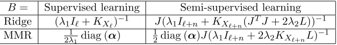
B = Supervised learning Semi-supervised learning Ridge (λ1I`+KX`)

−1 _J(λ1I

`+n+KX`+n(J

T_{J + 2λ2L))}−1

MMR _2λ1

1diag (α)

1

2diag (α)J(λ1I`+n+ 2λ2KX`+nL)

−1

Table 2: Matrix B of the models obtained using the identity decomposable kernel in the

case of different settings and loss functions.

whereLy` =D`−A` is the graph Laplacian, withD` the diagonal matrix of degrees. The

kernel trick allows to work as if we have chosen the subspace spanned by _{e1, . . . ,e`}, the

eigenvectors of the matrix KY` as a feature space with an associated feature map that

verifies:

∀i∈ {1, . . . , `}, ϕy(ui) = [√γ1ei1, . . . , √

γ`ei`]T.

The kernel κy :U × U →R, also verifies:

∀i, j∈ {1, . . . , `}, κy(ui, uj) = (KY`)i,j.

In practise, we only need to knowKY`. Regarding the operator-valued kernel, we consider

here the identity decomposable kernel:

∀(u, u0)_{∈ U × U},_Kx(u, u0) =κx(u, u0)I.

We underline that even if this kernel may seem simple, we must be aware that in this task, we do not have the explicit expressions of outputsϕy(u) and prediction inFyis not the

final target. Therefore this operator-valued kernel allows us to work properly with output Gram matrix values.

Of particular interest for us is the expression of the scalar product which is the only one we need for link prediction. When using the identity decomposable kernel, the approxima-tion of the output kernel can be written as follows:

c

κy(u, u0) =hˆh(u),ˆh(u0)iFy = (κ

u x,U`)

T_BT_K Y`Bκ

u0

x,U`, (13)

whereB is a matrix of size`×`that depends of the loss function used (see Table 2). In the semi-supervised setting, the approximated output kernel has a similar expression, where

κu

x,U`,κ

u0

x,U` are replaced by κ

u

x,U`+n,κ

u0

x,U`+n and B is a matrix of size (`+n)×`. We can

notice that we do not need to know the explicit expressions of outputs ϕy(u) to compute

this scalar product. Besides, the approximation of the scalar producthϕy(u), ϕy(u0)iFy can

be interpreted as a modified scalar product between the inputsϕx(u) andϕx(u0).

5.2 Multi-Task Learning

(Caruana, 1997; Evgeniou et al., 2005). Examples of multi-task learning problems can be found in document categorization as well as in protein functional annotation prediction. Dependencies among target variables can also be encountered in the case of multiple re-gression.

We consider here the case of learningdtasks having the same input and output domains.

Evgeniou et al. (2005) have shown that this problem is equivalent to learning a vector-valued

functionh:_{X → Y} withdcomponentshi:_{X → Y}i using the vector-valued RKHS theory.

A natural way to integrate the task relatedness with operator-valued kernels is to use the decomposable kernels introduced in Subsection 3.4: _Kx(x, x0) =κx(x, x0)A. Several values

for the matrix A have been proposed (Evgeniou et al., 2005; Sheldon, 2008; Baldassarre

et al., 2012) based on the fact that the regularization term in the RKHS associated to a

decomposable OVK can be expressed in function ofA:

khk2

H= d

X

i,j=1

A†_i,jhhi, hjiH_κx,

where† denotes the pseudoinverse and Hκx the RKHS associated to the scalar kernel κx.

In the IOKR framework, the task structure can be encoded in two different ways. We can use a decomposable OVK in input as described previously and define a regularization term that will penalize thedcomponents of the functionhaccording to the task structure. Another way is to modify the output representation by defining an output kernel that will integrate the task structure. We propose to compare the three following models to solve multi-task learning with our framework:

• Model 0: κy(y,y0) =yTy0, with the identity kernelKx(x, x0) =κx(x, x0)I,

• Model 1: κy(y,y0) =yTA1y0, with the identity kernelKx(x, x0) =κx(x, x0)I,

• Model 2: κy(y,y0) =yTy0, with the decomposable kernel Kx(x, x0) =κx(x, x0)A2.

In the first case, the different tasks are learned independently :

∀x_{∈ X},ˆh0(x) =Y`J λ1I`+n+KX`+n(J

T_{J+ 2λ}

2L)

−1 κx_X

`+n,

while in the other cases, the tasks relatedness is taken into account :

∀x_{∈ X},ˆh1(x) =

p

A1Y`J λ1I`+n+KX`+n(J

T_{J + 2λ}

2L)

−1 κx_X

`+n,

∀x_{∈ X},ˆh2(x) =

d

X

j=1

γjejeTjY`J(λ1I`+n+γjKX`+n(J

T_{J+ 2λ}

2L))−1κxX`+n,

whereγj and ej are the eigenvalues and eigenvectors ofA2.

We consider a matrix M of size d_×dthat encodes the relations existing between the

different tasks. This matrix can be considered as the adjacency matrix of a graph between

tasks. We note LM the graph Laplacian associated to this matrix. The matrices A1 and

A2 are defined as follow:

A1 =µM+ (1−µ)Id,

whereµ is a parameter in [0,1].

The matrixA2was proposed by Evgeniou et al. (2005) and Sheldon (2008) for multi-task

learning from the following regularizer:

kh2_k2H=

µ 2

d

X

i,j=1

Mijkhi2−h

j

2k 2_{+ (1}

−µ)

d

X

i=1 khi_2k2.

This regularization term forces two tasks hi₂ and hj₂ to be close to each other when the similarity valueMij is high and conversely.

6. Numerical Experiments

In this section, we present the performances obtained with the IOKR approach on two differ-ent problems: link prediction and multi-task regression. In these experimdiffer-ents, we examine the effect of the smoothness constraint through the variation of its related hyperparameter

λ2, using supervised method as a baseline. We evaluate the method in the transductive

setting, in which the goal is to predict the correct outputs for the unlabeled examples, as well as in the semi-supervised setting.

6.1 Link Prediction

For the link prediction problem, we considered experiments on three datasets: a collection of synthetic networks, a co-authorship network and a protein-protein interaction (PPI) network.

6.1.1 Protocol

For different percentages of labeled nodes, we randomly selected a subsample of nodes as labeled nodes. We split the remaining nodes in two subsets: one containing the unlabeled nodes and another containing the test nodes. Labeled interactions correspond to interac-tions between two labeled nodes. This means that when 10% of labeled nodes are selected, it corresponds to only 1% of labeled interactions. The performances were evaluated by av-eraging the areas under the ROC curve and the precision-recall curve (denoted AUC-ROC and AUC-PR) over ten random choices of the labeled set. A Gaussian kernel was used for the scalar input kernelκx. Its corresponding bandwidth σ was selected by a leave-one-out

cross-validation procedure on the training set to maximize the AUC-ROC, jointly with the hyperparameterλ1. In the case of the least-squares loss function, we used the leave-one-out estimates approach introduced in Section 4. The output kernel used is a diffusion kernel

of parameterβ. Another diffusion kernel of parameter β2 was also used for the smoothing

penalty: exp(₋β2L) =P∞i=0

(−β2L)i

i! , whereLis the Laplacian ofW. Preliminary runs have

shown that the values of β and β2 have a limited influence on the performances, we then

have set both parameters to 1. Finally we set W toKX`+n.

6.1.2 Synthetic Networks

the improvement brought by the semi-supervised method in extreme cases, i.e. when the percentage of labeled nodes is very low.

The output networks were obtained by sampling random graphs containing 700 nodes

from a Erd˝os-Renyi law with different graph densities. The graph density corresponds to

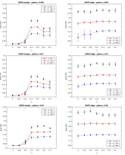
the probability of presence of edges in the graph. In this experiment we chose three densities that are representative of real network densities: 0.007, 0.01 and 0.02. For each network, we used the diffusion kernel on the full graph as output kernel and chose the diffusion parameter such that it maximizes an information criterion. To built an input kernel corresponding to a good approximation of the output kernel, we applied kernel PCA on the output kernel and derived input vectors from the truncated basis of the first components. We can control the quality of the input representation by varying the relative inertia captured by the first components. We then build a Gaussian kernel based on these inputs.

Figures 3 and 4 report respectively the averaged values and standard deviations for the AUC-ROC and AUC-PR obtained for different network densities and different percentages of labeled nodes in the transductive setting. IOKR-ridge corresponds to IOKR with a least-square loss and IOKR-margin to the hinge loss used in MMR. For these results, we used the components capturing 95% of the variance for defining the input vectors. We observe that IOKR-ridge outperforms IOKR-margin in the supervised and in the semi-supervised cases. This improvement is particularly significant for AUC-PR, especially when the network den-sity is strong and the percentage of labeled data is high. It is thus very significant for 10% and 20% of labeled data. In the supervised case, this observation can be explained by the difference between the complexities of the models. As shown in Equation (13), the solution obtained in the supervised case writes as: κ_cy(u, u0) = (κux,U`)

T_BT_K Y`Bκ

u0

x,U`. In Table 2,

we can see that the matrixB is only a diagonal matrix in the case of IOKR-margin whileB

is a full matrix for IOKR-ridge. This can also be seen in the dual optimization problem for

a general loss function (see Appendix B), where we observe that the dual variables αi are

simply collinear to the vector ˜yi for IOKR-margin. The synthetic networks may therefore

require a more complex predictor.

We observe an improvement of the performances in terms of AUC-ROC and AUC-PR for both approaches in the semi-supervised setting compared to the supervised setting. This improvement is more significant for IOKR-margin. This can be explained by the fact that the IOKR-margin models obtained in the supervised and in the semi-supervised cases do not

have the same complexity. As shown in Table 2, the matrixB of the IOKR-margin model

is a much richer matrix in the semi-supervised setting than in the supervised setting where it corresponds to a diagonal matrix. For IOKR-ridge, the improvement of the performance is only observed for low percentages of labeled data. We can therefore make the assumption that for this model, using unlabeled data increases the AUCs for low percentages of labeled data. But when enough information can be found in the labeled data, semi-supervised learning does not improve the performance. Based on these results, we can also formulate the assumption that link prediction is harder in the case of dense networks.

In Appendix C we experimented how the method behaves with perfect to noisy input features. We chose different levels of inertia (75%, 85%, 95% and 100%) for defining the input features. The results obtained with IOKR-ridge and IOKR-margin are shown in Table

8. We also include results on synthetic networks generated using mixtures of Erd˝os-Renyi

0 1e-6 1e-5 1e-4 1e-3 1e-2 1e-1 λ₂ 0.65 0.7 0.75 0.8 0.85 0.9 0.95 1 AUC-ROC

IOKR-margin - pdens = 0.007

p = 5% p = 10% p = 20%

0 1e-6 1e-5 1e-4 1e-3 1e-2 1e-1 λ₂ 0.65 0.7 0.75 0.8 0.85 0.9 0.95 1 AUC-ROC

IOKR-ridge - pdens = 0.007

p = 5% p = 10% p = 20%

0 1e-6 1e-5 1e-4 1e-3 1e-2 1e-1

λ₂ 0.65 0.7 0.75 0.8 0.85 0.9 0.95 1 AUC-ROC

IOKR-margin - pdens = 0.01

p = 5% p = 10% p = 20%

0 1e-6 1e-5 1e-4 1e-3 1e-2 1e-1

λ₂ 0.65 0.7 0.75 0.8 0.85 0.9 0.95 1 AUC-ROC

IOKR-ridge - pdens = 0.01

p = 5% p = 10% p = 20%

0 1e-6 1e-5 1e-4 1e-3 1e-2 1e-1 λ₂ 0.6 0.65 0.7 0.75 0.8 0.85 0.9 0.95 1 AUC-ROC

IOKR-margin - pdens = 0.02

p = 5% p = 10% p = 20%

0 1e-6 1e-5 1e-4 1e-3 1e-2 1e-1

λ₂ 0.6 0.65 0.7 0.75 0.8 0.85 0.9 0.95 1 AUC-ROC

IOKR-ridge - pdens = 0.02

p = 5% p = 10% p = 20%

0 1e-6 1e-5 1e-4 1e-3 1e-2 1e-1 λ₂ 0 0.05 0.1 0.15 0.2 0.25 0.3 0.35 0.4 0.45 AUC-PR

IOKR-margin - pdens = 0.007

p = 5% p = 10% p = 20%

0 1e-6 1e-5 1e-4 1e-3 1e-2 1e-1

λ₂ 0 0.05 0.1 0.15 0.2 0.25 0.3 0.35 0.4 0.45 AUC-PR

IOKR-ridge - pdens = 0.007

p = 5% p = 10% p = 20%

0 1e-6 1e-5 1e-4 1e-3 1e-2 1e-1 λ₂ 0 0.05 0.1 0.15 0.2 0.25 0.3 0.35 0.4 0.45 0.5 AUC-PR

IOKR-margin - pdens = 0.01

p = 5% p = 10% p = 20%

0 1e-6 1e-5 1e-4 1e-3 1e-2 1e-1 λ₂ 0 0.05 0.1 0.15 0.2 0.25 0.3 0.35 0.4 0.45 0.5 AUC-PR

IOKR-ridge - pdens = 0.01

p = 5% p = 10% p = 20%

0 1e-6 1e-5 1e-4 1e-3 1e-2 1e-1

λ₂ 0 0.05 0.1 0.15 0.2 0.25 0.3 0.35 0.4 0.45 AUC-PR

IOKR-margin - pdens = 0.02

p = 5% p = 10% p = 20%

0 1e-6 1e-5 1e-4 1e-3 1e-2 1e-1

λ₂ 0.05 0.1 0.15 0.2 0.25 0.3 0.35 0.4 0.45 AUC-PR

IOKR-ridge - pdens = 0.02

p = 5% p = 10% p = 20%

6.1.3 NIPS Co-authorship Network

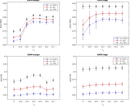
We applied our method on a co-authorship network containing information on publications of the NIPS conferences between 1988 to 2003 (Globerson et al., 2007). In this network, vertices represent authors and an edge connects two authors if they have at least one NIPS publication in common. Among the 2865 authors, we considered the ones with at least two links in the co-authorship network in order to have a significant density and try to keep close to the original data. We therefore focused on a network containing 2026 authors with an empirical link density of 0.002. Each author was described by a vector of 14036 values, corresponding to the frequency with which he uses each given word in his papers.

Figure 5 reports the averaged AUC-ROC and AUC-PR obtained on the NIPS co-authorship network in the transductive setting for different values of λ2 and different per-centages of labeled nodes. As previously, we observe that the semi-supervised approach

0 1e-6 1e-5 1e-4 1e-3 1e-2 1e-1

λ₂

0.65 0.7 0.75 0.8 0.85 0.9 0.95

AUC-ROC

IOKR-margin

p = 2.5% p = 5% p = 10%

0 1e-6 1e-5 1e-4 1e-3 1e-2 1e-1

λ₂

0.65 0.7 0.75 0.8 0.85 0.9 0.95

AUC-ROC

IOKR-ridge

p = 2.5% p = 5% p = 10%

0 1e-6 1e-5 1e-4 1e-3 1e-2 1e-1

λ₂

0.05 0.1 0.15 0.2 0.25 0.3

AUC-PR

IOKR-margin

p = 2.5% p = 5% p = 10%

0 1e-6 1e-5 1e-4 1e-3 1e-2 1e-1

λ₂

0.05 0.1 0.15 0.2 0.25 0.3

AUC-PR

IOKR-ridge

p = 2.5% p = 5% p = 10%

AUC-ROC AUC-PR

p 5% 10% 20% 5% 10% 20%

Transductive setting

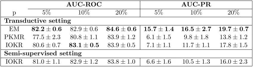
EM 87.3_±2.4 92.9_±1.7 96.4_±0.8 13.8_±4.5 22.5_±6.6 41.1_±2.5 PKMR 85.7_±4.1 92.4_±1.6 96.4_±0.4 9.7_±2.8 20.0_±4.8 38.8_±2.0 IOKR 83.6±5.9 93.6±1.0 96.5±0.4 12.0±3.0 24.5±2.9 43.7±1.9 Semi-supervised setting

IOKR 86.0_±2.7 93.3_±0.7 95.7_±1.4 7.6_±2.3 13.8_±1.7 25.3_±3.0

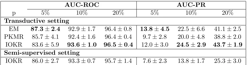
Table 3: AUC-ROC and AUC-PR obtained for the NIPS co-authorship network inference with EM, PKMR, IOKR in the transductive setting, and with IOKR in the semi-supervised setting. p indicates the percentage of labeled examples.

improves the performances compared to the supervised one for both models. For AUC-ROC values, this improvement is especially important when the percentage of labeled nodes is low. Indeed, with 2.5% of labeled nodes, the improvement can reach in average up to 0.14 points of AUC-ROC for IOKR-margin and up to 0.11 points for IOKR-ridge. As for the synthetic networks, the IOKR-ridge model outperforms IOKR-margin model in terms of AUC-ROC and AUC-PR, especially when the proportion of labeled examples is large. The explanation provided for the synthetic networks regarding the complexity of the solu-tions for IORK-margin and IOKR-ridge holds here also. In the following, we will focus on IOKR-ridge only.

We compared IOKR-ridge with two transductive approaches: the EM-based approach (Tsuda et al., 2003; Kato et al., 2005) and Penalized Kernel Matrix Regression (PKMR) (Yamanishi and Vert, 2007). These two methods regard the link prediction problem as a

kernel matrix completion problem. The EMmethod fills the missing entries of the output

Gram matrix KY by minimizing the information geometry, as measured by the

Kullback-Leibler divergence, with the input Gram matrix KX. The PKMR approach considers the

kernel matrix completion problem as a regression problem between the labeled input Gram

matrixKX`and the labeled output Gram matrixKY`. We did not compare our method with

the Link Propagation framework (Kashima et al., 2009) because this framework assumes that arbitrary interactions may be considered as labeled while IOKR requires a known subgraph. 500 examples were used for the test set and the remaining 1526 examples for the training set, which corresponds to the union of the labeled and unlabeled sets. For the labeled set we used 5%, 10% and 20% of the training examples and the left examples for the unlabeled set. We averaged the AUC over ten random partitions of the examples in labeled/unlabeled/test sets. The hyperparameters were selected by a 5-CV experiment on the labeled set for the three methods. The hyperparameters were selected separately

for the AUC-ROC and the AUC-PR. For IOKR, we selected also the λ2 parameter in this

experiment, and we sparsified the matrixW in the semi-supervised constraint using 10% of

thek-nearest-neighbors.

setting as the other methods are transductive. We observe that IOKR obtains better AUC-ROC and AUC-PR than EM and PKMR when the percentage of labeled data is greater or equal than 10%. For 5% the best performing method is the EM approach. Regarding the results of IOKR in the semi-supervised setting, we observe that the AUC-ROC results stay relatively similar compared to the transductive setting. However the AUC-PR values decrease significantly between the transductive and the semi-supervised settings. Consider-ing the proteins for which we want to predict the interactions in the continuity constraint seems to help a lot the performances in term of AUC-PR.

6.1.4 Protein-Protein Interaction Network

We also performed experiments on a protein-protein interaction (PPI) network of the yeast Saccharomyces Cerevisiae. This network was built using the DIP database (Salwinski et al., 2004), which contains protein-protein interactions that have been experimentally deter-mined and manually curated. We used more specifically the high confidence DIP core subset of interactions (Deane et al., 2002). For the input kernels, we used the annotations provided by Gene Ontology (GO) (Ashburner et al., 2000) in terms of biological processes, cellular components and molecular functions. These annotations are organized in three different ontologies. Each ontology is represented by a directed acyclic graph, where each node is a GO annotation and edges correspond to relationships between the annotations, like sub-class relationships for example. A protein can be annotated to several terms in an ontology. We chose to represent each proteinui by a vector si, whose dimension is equal to

the total number of terms in the considered ontology. If a protein ui is annotated by the

termt, then :

s(_it)=₋ln

number of proteins annotated byt

total number of proteins

.

This encoding allows to take into account the specificity of a term in the ontology. We then used these representations to built a Gaussian kernel for each GO ontology. By considering the set of proteins being annotated for each input kernel and being involved in at least one physical interaction, we obtained a PPI network containing 1242 proteins.

Based on the previous numerical results, we chose to consider only IOKR-ridge in the following experiments. We compared our approach to several supervised methods proposed for biological network inference:

• Naive (Yamanishi et al., 2004): this approach predicts an interaction between two proteins u andu0 ifκx(u, u0) is greater than a threshold θ.

• kCCA (Yamanishi et al., 2004): kernel CCA is used to detect correlations existing

between the input kernel and a diffusion kernel derived from the adjacency matrix of the labeled PPI network.

• kML (Vert and Yamanishi, 2005): kernel Metric Learning consists in learning a new

metric such that interacting proteins are close to each other, and conversely for non interacting proteins.

• OK3+ET(Geurts et al., 2006, 2007a): Output Kernel Tree with extra-trees is a tree-based method where the output is kernelized and is combined with ensemble methods.

The pairwise kernel method (Ben-Hur and Noble, 2005) was not considered here because this method requires to define a Gram matrix between pairs of nodes, which raises some practical issues in terms of computation time and storage. However we could have used an online implementation of the pairwise kernel method like the one used in Kashima et al. (2009) and thus avoid to store the large Gram matrix.

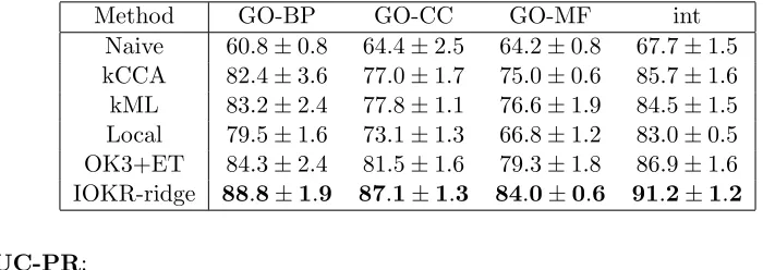
Each method was evaluated through a 5-fold cross-validation (5-CV) experiment and the hyperparameters were tuned on the training fold using a 4-CV experiment. As the local method can not be used for predicting interactions between two proteins of the test set, AUC-ROC and AUC-PR were only computed for the prediction of interactions between proteins in the test set and proteins in the training set. Input kernel matrices were defined for GO ontology and an integrated kernel, which was obtained by averaging the three input kernels, was also considered. Table 4 reports the results obtained for the comparison of the different methods in the supervised setting. We can see that output kernel regression based methods work better on this dataset than the other methods. In terms of AUC-ROC, the IOKR-ridge method obtains the best results for the four different input kernels, while for AUC-PR, OK3 with extra-trees presents better performances. We also compared the

aver-a) AUC-ROC:

Method GO-BP GO-CC GO-MF int

Naive 60.8_±0.8 64.4_±2.5 64.2_±0.8 67.7_±1.5 kCCA 82.4_±3.6 77.0_±1.7 75.0_±0.6 85.7_±1.6 kML 83.2±2.4 77.8±1.1 76.6±1.9 84.5±1.5 Local 79.5_±1.6 73.1_±1.3 66.8_±1.2 83.0_±0.5 OK3+ET 84.3_±2.4 81.5_±1.6 79.3_±1.8 86.9_±1.6 IOKR-ridge 88.8±1.9 87.1±1.3 84.0±0.6 91.2±1.2

b) AUC-PR:

Method GO-BP GO-CC GO-MF int

Naive 4.8_±1.0 2.1_±0.6 2.4_±0.4 8.0_±1.7

kCCA 7.1±1.5 7.7±1.4 4.2±0.5 9.9±0.4

kML 7.1_±1.3 3.1_±0.6 3.5_±0.4 7.8_±1.6

Local 6.0_±1.1 1.1_±0.3 0.7_±0.0 22.6_±6.6 OK3+ET 19.0±1.8 21.8±2.5 10.5±2.0 26.8±2.4 IOKR-ridge 15.3_±1.2 20.9_±2.1 8.6_±0.3 22.2_±1.6

Table 4: AUC-ROC and AUC-PR estimated by 5-CV for the yeast PPI network reconstruc-tion in the supervised setting with different input kernels (GO-BP: GO biological

processes; GO-CC: GO cellular components; GO-MF: GO molecular functions;