On the Jitter Sensitivity of an Adaptive Digital Controller: A Computational Simulation Study

On the Jitter Sensitivity of an Adaptive Digital Controller:

A Computational Simulation Study

Michael Short

, Fathi Abugchem

School of Science, Engineering and Design, Teesside University, Middlesbrough, UK

Received 09 April 2019; received in revised form 05 June 2019; accepted 20 June 2019

Abstract

In many real-time control applications, the ability to accurately track a reference trajectory with stable, pre-specified closed-loop dynamics is highly desirable. For fixed gain control systems, the detrimental impact of jitter on performance has been relatively well studied. However, research that quantifies the possible impact of jitter on the performance and relative stability of adaptive control schemes is comparatively much rarer. With technology advances now making real-time adaptive control a viable option for high-speed applications, this situation requires further investigation. In this paper, the jitter sensitivity of a digital parameter adaptive tracking control system is studied using precise software-in-the-loop computational simulations. The results obtained indicated that the adaptive controller was significantly susceptible to jitter. In particular, key metrics such as the phase margin, gain margin, settling time, overshoot and root mean square parameter and tracking errors were all significantly impacted following the introduction of 5% jitter in the controller. The obtained data are thought to be the first detailed results of this kind and present useful insights into the practical complexities when innovating adaptive real-time tracking control systems and indicate that specialized controller implementations that minimize jitter should be employed and that further analysis is warranted.

Keywords: adaptive control, digital control, digital signal processing, timing jitter

1.

Introduction

Many real-time control applications such as robotics benefit greatly from the ability to accurately track a reference trajectory with stable, pre-specified target dynamics. For digital control systems featuring fixed structure and gains, e.g. such as can be found in traditional robot controllers, the detrimental impact of jitter on performance has been relatively well studied. However, in practice, the dynamics of a controlled system may vary or change with time for one of several reasons: the nonlinearity of the plant dynamics, the use of reduced-order approximations to obtain locally linear models, and changes in the operational environment such as temperature, wear-and-tear, etc. [1-5]. This motivates the use of a variable structure or adaptive controls. For example, the dynamics of each axes of a multiple Degree-of-Freedom (DoF) robot manipulators are highly nonlinear, being coupled by the overall manipulator position, velocity, and acceleration; they are also dependent upon the payload mass, which can be variable and is highly application-dependent [4-5]. Similar effects can be found in other application domains: temperature control systems, for example, have been found to benefit from adaptive control; aircraft operate over a wide range of speeds and altitudes, their dynamics are highly nonlinear and are dependent upon velocity, acceleration, and altitude. Adaptive control is designed to cope with such variability and/or uncertainty in the dynamics of the controlled system; in general, an adaptive controller will continually update its behavior in real-time to adapt to changes in the dynamics of the plant and maintain a nominal closed-loop performance specification. Although adaptive control has

been widely studied during the past decades for applications such as the design of autopilots for high-performance aircraft, temperature control systems, wastewater treatment and motion control systems e.g. robotics, it is only with relatively recent technological and algorithmic advances that real-time adaptive control has become a viable option for high-speed embedded applications.

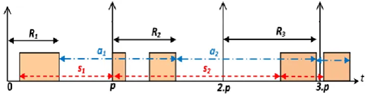
Adaptive control implementations, like all digital control implementations, may be susceptible to timing jitter. Although ideal timing models for sampling/actuation are apriori assumed for design purposes [5-6], jitter is an implementation issue that cannot be ignored in real-world implementations. There are multiple possible sources of timing jitters; a typical source of jitter is that which can be induced by an underlying real-time operating system. In a multi-tasking environment, the presence of multiple computational tasks with different (possibly time-varying) priorities can lead to task scheduler interference, as depicted in Fig. 1.

Fig. 1 Schedule-induced task execution jitter

Fig. 1 shows three instances of a periodic control task, requiring some finite computational resources for its execution (shaded area) once every p seconds. Although the task may be made ready once every p seconds without variation, due to pre-emptions from higher priority tasks that may also be pending (and possible variations in their execution times), the effective time differences between the starting time sk and completion time ak (where k is the instance number) of the execution of the different instances can be highly variable. Due to the presence of this scheduler-induced delay and jitter, the execution of task instances is not equidistant, and that the task response times Rk are not uniform. There are clearly implications for such variations if tasks are concerned with input sampling, control calculations and output refreshing in a real-time control system.

implementation is explored in much greater depth to provide such an in-depth investigation. In particular, the following two research questions are investigated: Q1: What is the impact of adding 5% random sampling jitter in a representative real-time adaptive controller on the tracking performance of the closed-loop? Q2: What is the impact of adding 5% random sampling jitter in a representative real-time adaptive controller on the relative stability of the closed loop?

In order to carry out the investigations, detailed Software-In-The Loop (SIL) simulations - using a representative digital parameter-adaptive controller and time-varying process model, have been employed. The SIL simulations were employed to compare a benchmark (no-jitter) implementation with an implementation in which a random jitter (corresponding to 5% of control period) was emulated in the control implementation. During the simulations, a number of key metrics of closed-loop performance and stability were recorded, including the phase margin, gain margin, settling time, overshoot, RMS tracking error, and RMS parameter estimation errors. The findings obtained indicate that when this level of jitter was added into the implementation, all metrics were all influenced by significant margins compared to the jitter-free implementation. In fact, the controller was only able to re-tune to meet the desired performance specification following a change of process parameters 8.75% of the time when jitter was present, as compared to 100% of the time in the jitter-free case. The results form a significant observation, as a common design suggestion for real-time digital control and signal processing is that jitter should be controlled to not more than 10% of the sample period (with the sample period chosen appropriately), to minimize the impact on the implementation [16-18]. This design suggestion may even be conservative in practice, as [19] experimentally report no adverse impacts of 10% sampling jitter in a DSP system. The results obtained in this paper suggest that this rule seems not conservative and in fact inadequate, for adaptive digital control (especially for oscillatory processes) and adaptive digital filtering implementations. In such cases, it is comparatively more important to ensure that either jitter is engineered out of an adaptive controller implementation (well below the 5% level) or additional compensation is employed. The obtained data are thought to be the first detailed simulation results of this kind and present a useful insight into the practical complexities of the advanced real-time control system and adaptive filtering implementation and innovation. The remainder of this paper is structured as follows. Section 2 presents an analysis of jitter sources in a control loop and outlines the motivation for the simulation-based approach. Section 3 describes the environment employed for the computational simulations and the configuration which was employed. Section 4 presents results, while Section 5 describes their analysis. Section 6 concludes the paper and outlines areas for future work.

2.

Theoretical Background

As mentioned in the introduction, the analysis of the effects of jitter for digitally controlled continuous plant dynamics is a non-trivial exercise, even in the Single Input/Single Output (SISO) case with time-invariant plant and deterministic jitter sources. One of the most detailed analytical models for such a situation was developed by Boje using w-domain concepts [13]. Consider the w-domain transfer function, which is obtained directly from the bilinear transform:

2 1 1 2

,

1 1 2

z wT

w z

T z wT

 

 _  _ (1)

process and disturbance outputs respectively. In addition, γu(k) represents the instantaneous control delay and γy(k) represents the instantaneous sampling delay at sample k (note that to enforce determinism, it is assumed that at each index k the relationship 0  γu(k)  γy(k) < T holds), with mean delay components u and y respectively. From Fig. 2, it can be seen that both control and sampling jitter introduce two jitter-induced noise components that depend upon products of the rate of change of control and plant signals; in addition, an additional system component D(w) is added into the forward path:

1 ( 2 )

( )

1 2

u y

w wT D w

wT

 

  

 _ (2)

Fig. 2 Approximate equivalents open-loop plant with control jitter (γu(k)) andsampling jitter (γy(k)), reproduced from [13]

These approximations are accurate to O(T) and are satisfactory when the sampling rate is high compared to the bandwidth of the continuous plant. Although the developed models provide the basis for a stability and/or performance analysis to proceed, as noted by [13]:

“In practical problems, the uncertainty in sampling instants may be caused by a combination of deterministic and random events. Finding necessary and sufficient conditions for stability is likely to be an intractable problem and sufficiency-only results may be too conservative for practical use.”

“Accurate (probabilistic or deterministic) descriptions of the jitter and plant conditions will generally not be available, and attempting to find the distributions of signal products may not be rewarding even for open loop systems. Feedback loops and the correlation between measurement and control action jitter will further complicate analysis”

motivation to employ experimental methods to determine the impacts of jitter in a closed-loop adaptive digital control system; this forms the basis for the experimental approach considered in this paper and described in the next Section.

3.

Simulation-Based Experimental Methodology

In order to provide a comparative test of performance and stability of an adaptive controller both with and without jitter, two simulation-based experiments, each of duration four hours were performed and a number of key performance metrics were either directly recorded and/or calculated from recorded data. The controller, simulation environment, recorded metrics, and experimental configuration is described in the Sections below.

3.1. Adaptive controller

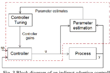
Adaptive controllers can be implemented using either direct or indirect approaches [1-3]; the latter is most commonly encountered and was chosen for the experiments. In an indirect approach, an estimation algorithm is first used to estimate the parameters of the controlled system on-line, and these parameters are used to calculate the controller gains [2]. A block diagram of the typical layout of a self-tuning indirect adaptive controller is as shown in Fig. 3. The adaptive controller in this context is formed by combining the on-line exponentially weighted recursive least squares (EW-RLS) algorithm with a discrete control law based on the direct design method proposed by Short et al. [21].

Fig. 3 Block diagram of an indirect adaptive controller

Suppose that the identified process model is given by the discrete transfer function G(z) = B(z)/A(z), where z = e(α+j)Ts is the z-transform shift operator with sample time Ts. The method proposed in [21] allows the synthesis of a predictive digital controller D(z) directly from the desired closed-loop pole specifications encoded in a design polynomial P(z). Under the assumption that B(z), the open loop numerator of the process (including the time delay and any zeros) is to be scaled and embedded in the closed-loop transfer function, the following controller design achieves the specification:

( ) (1)

( ) , with:

( ) ( ) (1)

p

p p

k A z P

D z k

P z k B z B

 

 (3)

The relation above was obtained by rearranging the characteristic equation of a process under unity negative feedback, with the scaling gain kp chosen to ensure that the closed-loop transfer function has unit gain and the controller contains an integrator. The advantages of embedding the open loop zeros of the process into the closed loop response are numerous and include the ability to adaptively track changes in the time delay without any explicit delay-estimation applied to the estimated polynomial B(z), and robustness against inverse response (unstable zeros) in the process. In the adaptive controller, the EW-RLS estimator is used to estimate the value of the process model parameters in real-time and is appropriate for use in embedded adaptive control applications in which the model dimension is not excessive. The derivation of the entire EW-RLS algorithm can be found in many previous works [22-23], and the main formulae for its implementation are:

ˆ_{( )t} ˆ_{(t 1) K t e t( ) ( )}

ˆ ( ) ( ) T( ) ( 1)

e t y t x t  t (5)

( 1) ( ) ( )

( ) ( 1) ( ) T

P t x t K t

x t P t x t

 



  (6)

1

( ) ( 1) ( ) T( ) ( 1)

P t __P t K t x t P t _ (7)

Where β(t) is the vector of estimated parameters of the system, y(t) is the current measured output of the system under consideration, x(t) is a vector of shifted previous input and output measurements of the system (regression variables), K(t) is the estimator gain vector, P(t) is the covariance matrix, e(t) is the prior residual error and  is the forgetting factor. In the experiments described in this paper, a fixed forgetting factor (of value described in Section 3.3 below) was employed. At each iteration, following the identification step to update the process parameter estimates, the controller gains were determined using equation 1 and the control signal calculated and applied. This gave a simple but effective and easily implementable means for implementing the adaptive controller.

3.2. Simulation environment

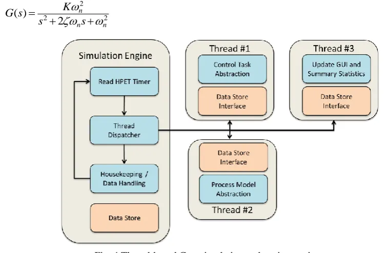
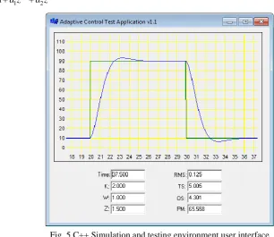
The EW-RLS estimator and the adaptive digital controller as described above were implemented in C++ code; in order to experiment with them, a software-based simulation and testing environment were required. In order to achieve this, a Windows-based PC application was created in C++ using Borland C++ Builder 6.0 © . The overall architecture of the application was as shown in Fig. 4. The main simulation engine executes in a loop and first reads a timestamp from the PC’s High-Precision Event Timer (HPET). The timestamp was then supplied to a local scheduler, which dispatched three threads at their respective start times. After dispatching the threads, some internal housekeeping was performed before looping to read the timer again. The three threads consisted of sequential code blocks concerned with updating the adaptive controller (#1), updating the time-varying process model (#2) and updating the recorded metrics and user interface (#3). Each thread exchanges data with the other threads through a small global data store. A screenshot of the test application user interface is shown in Fig. 5. In both experiments, the process to be controlled was assumed to be a 2nd order time-varying plant with static gain K, natural frequency n and damping ratio :

2

2 2

( )

2

n

n n

K

G s

s

s













Fig. 4 Thread-based C++ simulation and testing environment

system, or a chemical/thermal process. The reason for this is that such a process can model either over or underdamped behavior - along with the static gain and speed of response, of the dominant poles in the local approximation. After digitization at a given sample rate, an equivalent discrete linear model with two Auto-Regressive (AR) and two Moving Average (MA) parameters is obtained as y(t) + a1 y(t-1) + a2 y(t-2) = b1 u(t-1) + b2 u(t-2), having the discrete transfer

function:

1 2

1 2

1 2

1 2

( ) 1

b z b z G z

a z a z

 

 

 

  (9)

Fig. 5C++ Simulation and testing environment user interface

In order to obtain effective simulations, the process model was configured to have a sample rate 100 times faster than that of the controller sample rate. The process parameters were updated once every minute during the course of the experiments by making a small uniformly-distributed perturbation to each of the continuous model parameters, to achieve a drifting effect. After applying the perturbation, the continuous model was digitized to obtain the corresponding ARMA equation using the formulae provided in [24]. The upper and lower limits for gain K were 4.0 and 0.5 respectively, for natural frequency n were 4.0 and 0.5 respectively and for damping ratio  were and 2.0 and 0.1. For very high-speed applications, the natural frequency could be increased even further; however the choice of 4.0 as an upper limit was chosen to obtain an initial set of results, and further increases are left for future works. In each case, the maximum step size was set to  0.1. In total, 240 combinations of parameter values were tested in each experiment. An identical seed was employed in the random number generator to ensure consistency across parameter combinations in both experiments. During code development stages, known good practices were adhered to to minimize the risk of errors or defects impacting the simulations [25].

3.3. Experimental configuration

appropriate sampling time for the adaptive controller, the following methodology was employed. In addition to considerations on the closed-loop bandwidth and rise-time, a good rule-of-thumb is to set the sampling rate ts according to the measured open-loop rise time of the plant tr, such that ts ≤ tr/5. If this inequality is satisfied, then at least five samples will be processed by the controller during the transient period following a unit step change of the process input. A high-accuracy quadratic approximation to the rise-time of a second order system such as that above is given by [5]:

2

2.23

0.078

1.12

r

n

t







_





From which we observe that the rise time is inversely linearly proportional to the natural frequency for a fixed damping ratio, and for a fixed natural frequency, the rise time is directly proportional to the damping ratio. From Section 3.2, the maximum natural frequency (4.0) and minimum damping ratio (0.1) provide the boundary condition on the fastest rise time, which equates to tr = 0.284 seconds. The sample rate was accordingly set to T = 0.05 seconds (5.56 times the fastest rise-time) for the experiments. The process model abstraction was, therefore, run with sample rate TM = 0.0005 seconds. In the experiments, the adaptive controller was given a simple target specification for an optimally-damped pair of closed-loop poles with damping ratio  = ½ and natural frequency n = 1.303 rads/s was chosen. From basic control theory, the 99% settling time ts and peak overshoot OS of a second order system is related to these parameters according to the expressions [5]:

4.6

s n

t



_

2 1

100

OS

e



For the choices of  and n above, a 99% settling time ts = 5s and peak overshoot O/S = 4.321% are achieved by this specification. Although 95% and 98% settling times are also commonly used [5], the choice of 99% settling time and corresponding 1% settling band was made to provide for a tighter metric that may better expose any effects of jitter. The phase margin gives a measure of the relative stability of a closed loop system, and for a second-order closed-loop response is related to the damping ratio using the well-known relationship:

1

2 4

2

tan

2

1 4

PM











 

Peak Overshoot (OS) gives a measure of the damping and speed of rise-time in the closed loop design and is expressed as the maximum deviation over the final steady-state divided by the relative size of the step change in reference. The target overshoot for the choice of closed-loop damping ratio is 4.321%.

Settling Time (TS) is the time taken for the process output to achieve (and remain) within a 1% tolerance band of the commanded relative change in output. The settling time gives an indication of the closed-loop system natural frequency. The desired target for the settling time given the target closed-loop natural frequency and damping ratio is 5.000 seconds.

Phase Margin (PM) is the phase margin gives a measure of the relative stability of the closed-loop system and represents the amount of additional phase-shift that could be tolerated in the closed loop with stability still being guaranteed. The phase margin was calculated by first forming the forward-path transfer function H(z) = D(z)G(z), using the controller D(z) designed using the estimated process parameters and the process G(z) formed using the actual process parameters. The critical frequency g was then determined as the frequency satisfying |H(e-j)| = 0 dB and also having the largest negative

phase response H(e-j). Determining the frequencies satisfying the target magnitude was performed by carrying out a frequency sweep in the range 0 <  /T, i.e. up to the Nyquist frequency, followed by bisection. The phase margin (in degrees) is then given as PM = H(e-jg) + 180. If the process parameters are correctly identified, then the forward-path transfer function H(z) = D(z)G(z) effectively has the form:

1 2

1 2

1 2

1 1 2 2

( )

1 ( ) ( )

p p

p p

k b z k b z H z

p k b z p k b z

 

 

 

    (14)

Which is clearly dominated by the target closed-loop denominator polynomial P(z). Through the choice of the scaling gain kp, (14) has a static gain independent of the process gain K for a fixed  and n, as these parameters are linearly mapped to the b1 and b2 process parameters with K as a linear scale factor. Across all values of  and n, the achievable phase margin lies in the range 65.4 – 63.9.

Gain Margin (GM) is the gain margin gives a further measure of the relative stability of the closed-loop system and represents the amount of additional process gain that could be tolerated in the closed loop with stability still being guaranteed. The gain margin was calculated by determining the critical frequency g as the frequency satisfying H(e-j) =

-180 (modulo 360) having the lowest magnitude response H(e-j). The gain margin (in decibels) is then given as GM = 20 log10 (|H(e-jc)|). If the process parameters are correctly identified, then following the analysis above, across all values of 

and n, the achievable gain margin lies in the range 33.5 dB – 32.5 dB.

Root Mean Square Reference Tracking Error (eRMS): the standard deviation of the average difference (error) between the actual closed-loop response and the reference (desired) closed-loop response over the course of the 10-second step. The eRMS error gives a measure of the quality-of-fit of the closed loop response to its specification. Assuming the concerned setpoint change occurs at time tsp, then the RMS error was recorded as follows:

2 10 ( ( ) ( )) 10 sp sp t t

y t r t dt eRMS









where y(t) is the actual closed-loop response and r(t) is the reference closed-loop response obtained from the pole’s specification and the setpoint. Ideally, the target value of RMS would be zero: the larger the value of recorded eRMS, the lower the quality of control.

pRMS error gives a measure of the quality of the parameter estimates of the adaptive controller. Assuming the concerned setpoint change occurs at time tsp, then the pRMS error was recorded as follows:

2 2 2 2

1 1 2 2 1 1 2 2

10

ˆ

ˆ

_ˆ

_ˆ

( ( )

( ))

( ( )

( ))

( ( )

( ))

( ( )

( ))

10

sp

t

t

b t

b t

b t

b t

a t

a t

a t

a t

dt

pRMS

 

 





















where b1, b2, a1, and a2 are the actual process parameters from (9), and the accented equivalents are the estimated process

parameters. Ideally, the target value of pRMS would be zero: the larger the value of recorded pRMS, the lower the quality of the parameter estimates. The results obtained are described in the next Section.

4.

Simulation Results

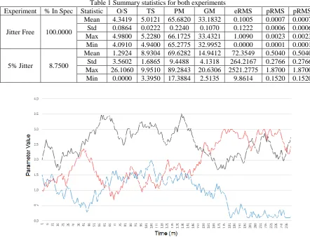
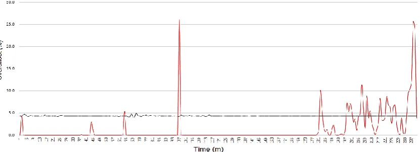
The evolution of the process parameters over the course of both experiments was as shown in Fig. 6. The recorded values of closed-loop Overshoot (OS), Settling time (TS), Phase Margin (PM), Gain Margin (GM), Root Mean Square Tracking Error (eRMS), and Root Mean Square Parameter Estimation Error (pRMS) are depicted in Figs. (7-12) for both jitter-free and 5% jitter cases. In all figures, time (in minutes) is represented on the horizontal axis, which the recorded metric value on the vertical. Note that the axes scales are identical in all comparisons save for the eRMS error, in which Fig. 11 displays log10(1+x) for each error point having value x due to the large difference in recorded values. Table 1 displays

summary statistics for each metric, including the mean, standard deviation, maximum and minimum recorded values. The Table also indicates the percentage of responses which could be considered “within specification,” i.e. having an overshoot, settling time, gain margin, and phase margin not more than 15% away from their respective target values.

Table 1 Summary statistics for both experiments

Experiment % In Spec Statistic O/S TS PM GM eRMS pRMS pRMS

Jitter Free 100.0000

Mean 4.3419 5.0121 65.6820 33.1832 0.1005 0.0007 0.0007 Std 0.0864 0.0222 0.2240 0.1070 0.1222 0.0006 0.0006 Max 4.9800 5.2280 66.1725 33.4321 1.0090 0.0023 0.0023 Min 4.0910 4.9400 65.2775 32.9952 0.0000 0.0001 0.0001

5% Jitter 8.7500

Mean 1.2924 8.9304 69.6282 14.9412 72.3549 0.5040 0.5040 Std 3.5602 1.6865 9.4488 4.1318 264.2167 0.2766 0.2766 Max 26.1060 9.9510 89.2843 20.6306 2521.2775 1.8700 1.8700 Min 0.0000 3.3950 17.3884 2.5135 9.8614 0.1520 0.1520

Fig. 7 Recorded value of closed-loop Overshoot (OS) during the two experiments (black: jitter-Free, red: 5% Jitter)

Fig. 8 Recorded value of closed-loop Settling Time (TS) during the two experiments (black: jitter-Free, red: 5% Jitter)

Fig. 9 Recorded value of Phase Margin (PM) during the two experiments (black: jitter-Free, red: 5% Jitter)

Fig. 11 Recorded value of RMS reference tracking error (black: jitter-Free, red: 5% Jitter)

Fig. 12 Recorded value of RMS parameter estimation error (black: jitter-Free, red: 5% Jitter)

5.

Observations and Discussion

Firstly, observing Fig. 6 it can be seen that a wide variety of parameter combinations were present during the experiments, with the process exhibiting both overdamped and underdamped behaviors while the natural frequency exhibits both slow and fast dynamics. The gain also fluctuates considerably, giving a complex series of process variations to fully test the adaptive controller. Turning attention now to performance issues and the impact of jitter, Fig. 7 shows that the percentage overshoot for the jitter-free implementation was consistently close to the target value (4.321%) in the absence of jitter; Table 1 confirms that the mean (4.342) was very close to the design specification, with low range (0.889) and very low standard deviation (0.086 %). Fig. 7 however also shows that in the presence of jitter, the percentage overshoot was consistently away from the target value; the mean in this case (1.292%) indicated very sluggish response on average, but with a high range (26.106) and high standard deviation (3.560%). In particular, it can be noted that the overshoot was significantly variable and mostly exceeded the specification from approx. 180 minutes into the simulation. Although some other shorter periods also proved problematic for the controller, referring to Fig. 6, this corresponds to the period with low damping present in the open-loop system.

range (6.556) and high standard deviation (8.424). Again it can be noted that the settling time was significantly variable and mostly exceeded the specification from approx. 180 minutes into the simulation. Although some other shorter periods also proved problematic for the controller, referring to Fig. 6, this again corresponds to the period with low damping present in the open-loop system. Interestingly, the period between approx. 30 and 50 minutes also exhibits a longer settling time, when the damping is at a low level (approx. < 0.5).

Concentrating now upon the phase margin, Fig. 9 shows that this metric for relative stability was consistently close to the target value (64.5) in the absence of jitter; Table 1 confirms that the mean (65.503) was very close to the design specification, with low range (1.194) and very low standard deviation (0.022). Fig. 9 again shows that the phase margin was consistently away from the target value in the presence of jitter; the mean in this case (69.628) indicated a higher stability margin on average, but with a high range (71.896) and high standard deviation (9.449). In particular, the phase margin dropped to a value as low as 17.388 towards the end of the experiment, indicating a significant lowering of the stability margin. The initial part of the experiment, up until approximately the 115th minute, featured phase margins consistently below the target value. Although the phase margin on average was increased after the introduction of jitter, a somewhat unexpected result, the variability was also increased significantly; having situations in which the phase margin could occasionally drop as low as 17% would be unacceptable 1n most circumstances, as a sudden shift in process parameters could lead to closed-loop instability.

Concentrating now upon the gain margin, Fig. 10 shows that this metric for relative stability was consistently close to the target value (32.5 dB) in the absence of jitter; Table 1 confirms that the mean (33.183 dB) was very close to the design specification, with low range (0.437 dB) and very low standard deviation (0.107 dB). Fig. 10 again shows that the gain margin was consistently away from the target value in the presence of jitter; the mean in this case (14.941 dB) indicated a lower stability margin on average, with range (18.117 dB) and high standard deviation (4.132 dB). In particular, the gain margin dropped to a value as low as 2.514 dB towards the end of the experiment, indicating a significant lowering of this stability margin at the same time as that of the phase margin. The gain margin was found to be consistently below the target value for the duration of the experiment.

Focusing now upon the RMS tracking error as shown in Fig. 11, it can be observed that without jitter the adaptive controller could consistently maintain very good performance in terms of the closed-loop step response. Table 1 confirms that the mean RMS error (0.100) was very low, with low range (1.009) and a very low standard deviation (0.122). The peak RMS error recorded was 1.009. In the presence of jitter, the RMS metric was degraded significantly as can be seen in Fig. 11. Table 1 confirms that the mean (72.355) was vastly increased, with a high range (2511.416) and high standard deviation (264.217). The peak RMS recorded, in this case, was 2521.277. Interestingly, the minimum RMS (9.861) was also significantly increased over the maximum RMS recorded without jitter. Finally, considering now the RMS parameter tracking error as shown in Fig. 12, it can be observed that without jitter the adaptive controller could consistently maintain very good performance in terms of parameter tracking. Table 1 confirms that the mean RMS error (7.4 x 10-4) was very low, with low range (2.2 x 10-3) and a very low standard deviation (5.9 x 10-4). The peak RMS error recorded was 0.002. In the presence of jitter, the RMS parameter tracking metric was degraded significantly. Table 1 confirms that the mean (0.504) was vastly increased, with a high range (1.718) and high standard deviation (0.277). The peak RMS recorded, in this case, was 1.870. Interestingly, the minimum RMS (0.152) was also significantly increased over the maximum RMS recorded without jitter.

this did not also correspond to the worst-case with respect to gain and phase margins, which occurred after approximately 233 minutes, during a period with low damping. Considering Figs. 6-8, 10, it can be noted that the overshoot, gain margin and settling time were all significantly impacted upon and displayed large variability during the period of approx. 180 minutes into the simulation until the end. As this corresponds to the period with low damping present in the open-loop system, it seems a reasonable conclusion that when the open-loop response of a process is oscillatory and underdamped, the presence of jitter leads to reductions of stability margins and unpredictable and highly variable overshoot and settling time.

In summary, considering Table 1, the tracking controller was only able to fully re-tune to meet the desired performance specification following a change of process parameters 8.75% of the time when 5% jitter was present, as compared to 100% of the time in the jitter-free case. Referring back to the two research questions posed in the introduction, the following insight can be provided. With respect to the relative stability of the closed loop, in this experiment, the addition of 5% random sampling jitter led to a gain margin which was significantly reduced (in terms of mean and worst-case) and with significantly increased variability (in terms of standard deviation). The addition of 5% random sampling jitter also led to a phase margin which was slightly increased (in terms of the mean), significantly reduced (in terms of worst-case) and with significantly increased variability (in terms of standard deviation). With respect to estimation and tracking ability of the closed loop, in this experiment the addition of 5% random sampling jitter led to parameter estimation errors which were significantly increased (in terms of mean and worst-case) and with significantly increased variability (in terms of standard deviation). The addition of 5% random sampling jitter also led to tracking errors which were significantly increased (in terms of mean and worst-case) and with significantly increased variability (in terms of standard deviation).

Relating the discussion back to the analysis of Section 2, it can be observed that as expected the impact of jitter was significantly worse when the speed of response of the system model was increased (e.g. underdamped with higher natural frequency). This reflects the fact that larger signal derivatives were present in the system output and control signals, which lead to larger jitter-dependent “noise” in the signals. In this case, the primary symptoms were a reduction in stability margins and increased clop-loop instability. In addition, when the speed of response of the system was slow (overdamped with lower natural frequency) but the process had high gain, the impact of jitter was again significantly worse. Again, larger signal derivatives were present in the system output and control signals, which also lead to larger jitter-dependent ‘noise’ in the signals. However, in this latter case, the primary symptoms were larger estimation and tracking errors. Together, these results and observations suggest that for adaptive control in the presence of jitter, the effects are highly complex to analyze and can manifest in subtly different ways depending upon the process characteristic. As mentioned in the introduction, a common design suggestion for real-time control and signal processing is to keep jitter below a level of 10% of the period for the implementation of a design. The results obtained here suggest that for adaptive control (especially for situations in which high signal derivatives may be present in the closed-loop system), this rule would prove to be inadequate, and it becomes vital to ensure that jitter is engineered out of an adaptive controller implementation in such a case. In particular, a jitter bound well below the 5% of period level would seem to be required. A suitable design for a scheduler to give low-jitter for one or more key sampling and control tasks in a resource-constrained real-time control system, along with an in-depth derivation of the required task timing analysis, can be found in [15].

6.

Conclusions

are thought to be the first empirical results of this kind and present useful insights into the practical complexities of implementing advanced real-time tracking control systems. It is suggested that where possible, designers and innovators of adaptive tracking controllers for applications such as high-speed servoing and robotics should aim to engineer low-jitter solutions from the outset of the design process. Further work will concentrate upon (1) extending the computational simulation analysis presented in this paper with the goal of providing insights into simpler noise approximations that may yield a pessimistic, but workable, analysis procedure for situations in which jitter cannot be avoided, (2) experimentally investigating the variation in performance and relative stability effects as jitter levels are varied employing real hardware and/or process plant, and (3) investigating the impacts of jitter on other advanced process control algorithms, e.g. Model Predictive Control (MPC) [26].

Conflicts of Interest

The authors declare no conflict of interest.

References

[1] K. J. Astrom and B. Wittenmark, Adaptive control, 2nded. Addison Wesley, 1995.

[2] J. S. Kumar and D. Sankar, “Implementation of adaptive embedded controller for a temperature process,” Advances in Technology Innovation, vol. 4, no. 2, pp. 94-104, March 2019.

[3] I. Nascu, I. Nascu, and G. Vlad, “Predictive adaptive control of an activated sludge wastewater treatment process,” Advances in Technology Innovation, vol. 1, no. 2, pp. 38-40, October 2016.

[4] M. Short and K. Burn, “A generic controller architecture for intelligent robotic systems,” Robotics and Computer Integrated Manufacturing, vol. 27, no. 2, pp. 292-305, 2012.

[5] R. C. Dorf and R. H. Bishop, Modern control systems, 10th ed. Englewood Cliffs, NJ: Prentice-Hall, 2004. [6] K. J. Astrom and B. Wittenmark, Computer-control systems: theory and design, 3rd ed. Prentice Hall, ISBN

0-13-314899-8, 1997.

[7] Y. Wu, G. Buttazzo, E. Bini, and A. Cervin, “Parameter selection for real-time controllers in resource-constrained systems,” IEEE Transactions on Industrial Informatics, vol. 6, no. 4, pp. 610-620, November 2010.

[8] J. Nilsson, B. Bernhardson, and B. Wittenmark, “Stochastic analysis and control of real-time systems with random time delays,” Automatica, vol. 34, no. 1, pp. 57-64, January 1998.

[9] G. Buttazzo and A. Cervin, “Comparative assessment and evaluation of jitter control methods,” Proceedings of the 15th International Conference on Real-Time Networks and Systems (RTNS), Nancy, France, 2007.

[10] A. Cervin, “Improved scheduling of control tasks,” Proceedings of the 11th Euromicro Conference on Real-Time Systems (ECRTS), York, England, June 1999, pp. 4-10.

[11] G. Buttazzo, “Research trends in real-time computing for embedded systems,” ACM SIGBED Review, vol. 3, no. 3, pp. 1-10, July 2006.

[12] A. A. Fröhlich, G. Gracioli, and J. F. Santos, “Periodic timers revisited: the real-time embedded system perspective,” Computers and Electrical Engineering, vol. 37, pp. 365-375, May 2011.

[13] E. Boje, “Approximate models for continuous-time linear systems with sampling jitter,” Automatica, vol. 41, no. 12, pp. 2091-2098, December 2005.

[14] F. Abugchem, M. Short, and D. Xu, “An experimental HIL study on the jitter sensitivity of an adaptive control system,” Proceedings of the 18th IEEE International Conference on Emerging Technologies & Factory Automation (ETFA), Italy, 2013.

[15] F. Abugchem, “A kernel level solution for jitter control in resource-constrained real-time control applications,” Ph.D. dissertation, Teesside University, UK, August 2016.

[16] M. J. Pont, Patterns for time-triggered embedded systems: building reliable applications with 8051 family of microcontrollers, Addison Wesley, 2001.

[17] A. J. Jerri, “The Shannon sampling theorem: its various extensions and applications: a tutorial review,” Proceedings of the IEEE, November 1977, vol. 65, no. 11, pp. 1565-1596.

[19] D. J. McKinnon, B. Karanayil, and C. Grantham, “Investigation of the effects of DSP timer jitter on the measurement of a PWM controlled inverter output voltage and current,” Proceedings of the 4th

IEEE International Power Electronics and Motion Control Conference, Xi’an, China, August 2004.

[20] F. Eisenbrand and T. Rothvoss, “Static-priority real-time scheduling: response time computation is NP-hard,” Proceedings of the IEEE Real-Time Systems Symposium (RTSS), Barcelona, Spain, November 2008, pp. 397-406. [21] M. Short, F. Abugchem, and U. Abrar, “Dependable control for distributed wireless control systems,” Electronics,

vol. 4, no. 4, pp. 857-878, November 2015.

[22] L. Ljung and T. Soderstrom, Theory and practice of recursive identification, MIT Press, 1983. [23] L. Ljung, System identification: theory for the user, 2nd ed. Prentice Hall, 1987.

[24] C. P. Neuman and C.S. Baradello, “Digital transfer functions for microcomputer control,” IEEE Transactions on Systems, Man and Cybernetics, vol. 9, no. 12, pp. 856-860, 1984.

[25] M. Short, “Development Guidelines for Dependable Real-Time Embedded Systems,” Proceedings of the IEEE/ACS International Conference on Computer Systems and Applications (AICCSA), Doha, Qatar, April 2008, pp. 1032 – 1039. [26] M. Short, “A simplified approach to multivariable model predictive control,” International Journal of Engineering and

Technology Innovation, vol. 5, no. 1, pp. 19-32, January 2015.

Copyright© by the authors. Licensee TAETI, Taiwan. This article is an open access article distributed under the terms and conditions of the Creative Commons Attribution (CC BY-NC) license