University of Windsor University of Windsor
Scholarship at UWindsor
Scholarship at UWindsor
Electronic Theses and Dissertations Theses, Dissertations, and Major Papers
2016
Linear-Phase FIR Digital Filter Design with Reduced Hardware
Linear-Phase FIR Digital Filter Design with Reduced Hardware
Complexity using Discrete Differential Evolution
Complexity using Discrete Differential Evolution
Muhammed Kunwar Rehan University of Windsor
Follow this and additional works at: https://scholar.uwindsor.ca/etd
Recommended Citation Recommended Citation
Rehan, Muhammed Kunwar, "Linear-Phase FIR Digital Filter Design with Reduced Hardware Complexity using Discrete Differential Evolution" (2016). Electronic Theses and Dissertations. 5763.
https://scholar.uwindsor.ca/etd/5763
Linear-Phase FIR Digital Filter
Design with Reduced Hardware
Complexity using Discrete
Differential Evolution
by
Kunwar Muhammed Rehan
A Thesis
Submitted to the Faculty of Graduate Studies
through the Department of Electrical and Computer Engineering in Partial Fulfillment of the Requirements for
the Degree of Master of Applied Science at the University of Windsor
Windsor, Ontario, Canada
2016
c
Linear-Phase FIR Digital Filter Design with Reduced Hardware Complexity using Discrete Differential Evolution
by
Kunwar Muhammed Rehan
APPROVED BY:
Dr. Guoqing Zhang
Department of Mechanical, Automotive and Materials Engineering
Dr. Huapeng Wu
Department of Electrical and Computer Engineering
Dr. Hon Keung Kwan, Advisor
Department of Electrical and Computer Engineering
Declaration of Originality
I hereby certify that I am the sole author of this thesis and that no part of this thesis has been published or submitted for publication.
I certify that, to the best of my knowledge, my thesis does not infringe upon anyones copyright nor violate any proprietary rights and that any ideas, techniques, quotations, or any other material from the work of other people included in my thesis, published or otherwise, are fully acknowledged in accordance with the standard referencing practices. Furthermore, to the extent that I have included copyrighted material that surpasses the bounds of fair dealing within the meaning of the Canada Copyright Act, I certify that I have obtained a written permission from the copyright owner(s) to include such material(s) in my thesis and have included copies of such copyright clearances to my appendix.
Abstract
Dedication
Acknowledgements
Table of Contents
Declaration of Originality iii
Abstract iv
Dedication v
Acknowledgements vi
List of Tables x
List of Figures xii
List of Acronyms xiv
1 Introduction to Digital Filter Design 1
1.1 Mathematical Representation of Digital Filters . . . 2
1.2 Filter Design Methodology and Specifications . . . 4
1.3 Motivation and Outline of Thesis . . . 8
2 Review of Filter Complexity Reduction Methods 11
2.1 Filter Complexity Reduction Technique . . . 11
2.2 Multiplierless Filter Design . . . 13
2.2.2 MCM Algorithms . . . 16
2.2.3 State of the Art . . . 20
Summary . . . 24
3 Optimization Methods 26 3.1 Selection of Optimization Method . . . 27
3.2 Linear Programming . . . 28
3.3 Differential Evolution Algorithm for Continuous Optimization . . . 31
3.4 Variations of Differential Evolution . . . 34
3.4.1 Variation in Mutation . . . 34
3.4.2 Adaptive Control Parameters . . . 34
3.5 Differential Evolution for Discrete Filter Optimization . . . 35
Summary . . . 38
4 Proposed Algorithm 39 4.1 Problem Formulation . . . 40
4.1.1 Joint Optimization Objective Function . . . 40
4.1.2 DEFDO Algorithm . . . 42
4.2 Algorithms Used In DEFDO . . . 45
4.2.1 Linear Programs Used in Filter Design . . . 45
4.2.2 Population Generation for Differential Evolution . . . 47
4.2.3 Modified RAG-n Algorithm . . . 52
4.2.4 Selection Operator for Differential Evolution . . . 53
4.2.5 Adaptive Search Space Reduction . . . 54
4.2.6 Computation Cost Reduction . . . 55
5 Design Examples and Results 59
5.1 Comparison of Variations of DE Algorithms . . . 59
5.2 Joint Optimization of Minimax Error and Hardware Complexity . . . 63
5.2.1 Empirical Determination of Filter Order and Wordlength . . . 63
5.2.2 Design Examples . . . 65
5.3 Hardware Synthesis . . . 81
5.3.1 Structure of Filter and Shift Add Network . . . 81
5.3.2 Filter Adders’ Topology . . . 81
5.4 Result Comparison . . . 86
5.4.1 Adder Cost Comparison: Approximate Methods . . . 86
5.4.2 Adder Cost Comparison: Deterministic Methods . . . 89
5.5 Design Algorithm Complexity Analysis . . . 91
Summary . . . 94
6 Conclusion and Future Scope 95 6.1 Conclusion . . . 95
6.2 Contribution of Thesis . . . 96
6.3 Future Scope . . . 97
References 99
List of Tables
1.1 Amplitude Response of Linear Phase FIR Filters . . . 5
1.2 FIR vs. IIR . . . 6
1.3 Automatic Zeros of Linear Phase FIR Filters . . . 7
3.1 Linear Program Setup . . . 30
4.1 Range of Filter . . . 44
4.2 Quantized Range of Filter . . . 49
5.1 Filter Specifications . . . 65
5.2 Emperical Determination of Filter Order and Wordlength . . . 66
5.3 Result For Filter G1 . . . 69
5.4 Result For Filter G1 . . . 70
5.5 Result For Filter Y1 . . . 71
5.6 Result For Filter Y1 . . . 72
5.7 Result For Filter A . . . 73
5.8 Result For Filter B . . . 74
5.9 Result For Filter L1. . . 76
5.10 Result For Filter C . . . 77
5.11 Band Pass and Band Stop Specifications . . . 78
5.12 Result For Band Pass Filter . . . 79
5.14 Full Adder Count for Filters . . . 86
5.15 Comparison With Approximate Methods . . . 89
5.16 Comparison With Deterministic Methods . . . 90
5.17 Time Analysis for Small Length Filters . . . 92
5.18 Design Statistics for Large Filters . . . 93
List of Figures
1.1 Filter Design Specifications. . . 6
2.1 Transposed Direct Form . . . 16
2.2 Shift and Add Network . . . 17
2.3 Filter Design Approach . . . 18
3.1 Pseudo Code for the Differential Evolution Algorithm . . . 32
3.2 Pseudo Code for Discrete Differential Evolution . . . 37
4.1 Pseudo Code for Population Generation(Small) . . . 50
4.2 Pseudo Code for Decoding to Bits . . . 50
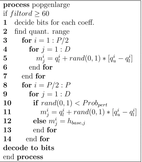
4.3 Pseudo Code for Population Generation(Large) . . . 51
4.4 Gray Encoding for Base Solution Neighborhood . . . 51
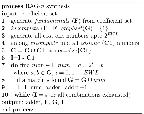
4.5 Pseudo Code for Synthesis Using RAG-n . . . 52
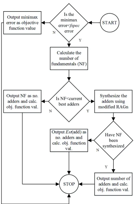
4.6 Selection Operation Flowchart . . . 54
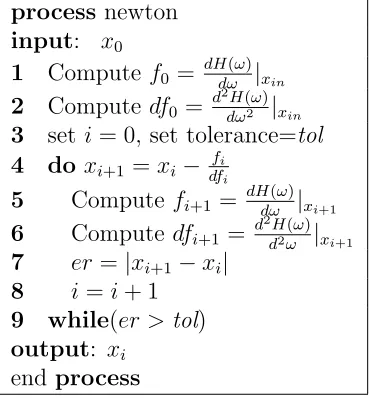
4.7 Pseudo Code for Extremal Points Using Newton’s Root Finding Algorithm 55 4.8 Pseudo Code for Newton’s Root Finding Algorithm . . . 56
4.9 Pseudo Code for Differential Evolution with Adaptive Search Space Reduc-tion and Pre-Calculated Objective FuncReduc-tion . . . 58
5.1 Convergence Curve for Different Value of F. . . 60
5.3 Convergence Curve for Adaptive and Fixed Control Parameters Before . . 61
5.4 Convergence Curve for Adaptive and Fixed Control Parameters After . . . 61
5.5 Convergence Curve for Different Variation of Mutation Operator . . . 62
5.6 Bar Graph Showing Filter Orders . . . 66
5.7 EWL vs. Filter Length for A. . . 67
5.8 EWL vs. Filter Length for B . . . 67
5.9 EWL vs. Filter Length for C . . . 68
5.10 Amplitude Response of Filter G1 (EWL=6) . . . 69
5.11 Amplitude Response of Filter G1 (EWL=7) . . . 70
5.12 Amplitude Response of Filter Y1 (EWL=9) . . . 71
5.13 Amplitude Response of Filter Y1 (EWL=10) . . . 72
5.14 Amplitude Response of Filter A . . . 73
5.15 Amplitude Response of Filter B . . . 74
5.16 Amplitude Response of Filter L1 . . . 75
5.17 Amplitude Response of Filter C . . . 75
5.18 Amplitude Response of Band Pass Filter . . . 79
5.19 Amplitude Response of Band Stop Filter . . . 80
5.20 Transposed Direct Form of Linear Phase FIR Filter with Multipliers Re-placed by Shift and Add Network . . . 81
5.21 Expanded Form of Filter G1 Synthesis . . . 82
5.22 Hardware Synthesis for Filter G1 (EWL=7) . . . 83
5.23 Synthesis of Shift Add Network for Filter Y1 (EWL=10) . . . 83
5.24 Ripple Carry Adder Topology for (a×2n+b) for n= 2 . . . . 84
5.25 Ripple Carry Adder Topology for (a×2n−b) for n= 2 . . . . 85
5.26 Comparison of Amplitude Response of Opitmal Finite Wordlength Design With Infinite Precision Parks McClellan Design for Filter A . . . 87
List of Acronyms
ACO Ant Colony Optimization
ASIC Application Specific Integrated Circuit
CR Crossover Rate
CSD Canonic Signed Digit
CSE Common Subexpression Elimination
DE Differential Evolution
DEFDO Differential Evolution Filter Design Optimization
EA Evolutionary Algorithms EWL Effective Word Length
F Mutation Factor FA Full Adder
FIR Finite Impulse Response
GA Genetic Algorithm GB Graph Based
HA Half Adder
LTI linear time invariant
MAD Maximum Adder Depth MBA Multiplier Block Adders
MCM Multiple Constant Multiplication MILP Mixed Integer Linear Programming
NPRM Normalized Peak Ripple Magnitude
PSO Particle Swarm Optimization
RAG-n Reduced Adder Graph-n
SA Structural Adders
SAN Shift and Add Network
Chapter 1
Introduction to Digital Filter Design
A digital filter is a system that alters an incoming signal in a desired way in order to extract useful information and discard undesirable components. Digital filters are used pervasively in wide ranging products. Some examples include:
• Communication Systems
• Digital Audio Systems
• Signal Processing Systems including applications in seismology, biology etc.
• Image Processing and enhancement systems
• Speech Synthesis
• Instrumentation and Control Systems
1.1
Mathematical Representation of Digital Filters
The emergence of digital technology in the 1960s opened a new world of applications. It was realized that digital filters have various advantages over their analog counterparts as
• Digital filters did not suffer from components tolerances and their response was in-variant to temperature and time.
• Digital filters could be programmed easily on digital hardware
• Digital filters were insensitive to electrical noise to a great extent
• Digital filters are very versatile in the desired responses they can produce
A digital filter can be characterized as a linear time invariant (LTI) discrete system. The LTI system can be described by a constant coefficient difference equation
y(n) =
N−1
X
k=0
a(k)x(n−k)− M
X
k=1
b(k)y(n−k)
where a(k) and b(k) are the forward tap coefficients and feedback tap coefficients respec-tively. Taking the z Transform of the above equation, and rearranging, we obtain the transfer function of the system shown in Eq. 1.1.
H(z) = Y(z) X(z) =
PN−1
k=0 a(k)z
−k
1 +PM
k=1b(k)z−k
(1.1)
From the Eq. 1.1, two sub classes of digital filters can be defined: Finite Impulse Re-sponse (FIR) filters, also called non recursive filters and Infinite Impulse ReRe-sponse (IIR) filters, also called recursive filters. Mathematically, the distinction is made for the case when poles are non existent in the transfer function. Hence, the denominator terms van-ishes and the transfer function can be written as
H(z) =
N−1
X
k=0
The above transfer function exhibits a finite length impulse response and hence is called the FIR filter transfer function.
Physically, the distinction is based on whether a feedback from the output exists or not. Recursive filters have a feedback from the output and hence possess impulse responses that are infinite in duration. A non-recursive or finite impulse response (FIR) digital filter, on the other hand, exhibits a finite duration impulse response. For an FIR filter whose impulse response of length1 N is given by h = [h
0, h1, h2· · ·hN−1]T the transfer function is found using the Z transform given by Eq. 1.2.
H(z) =
N−1
X
n=0
hnz−n (1.2)
The frequency response is defined as the transfer function evaluated atz =ejω. Hence,
the frequency response of a FIR digital filter can be written as in Eq. 1.3
H(ejω) =
N−1
X
n=0
hne−jωn (1.3)
The frequency response can be re-written as
H(ejω) =Ha(ω)θ(ω) (1.4)
where Ha(ω) = |H(ejω)| is called the magnitude response and and θ(ω) = ∠H(ejω) is
called the phase response. The group delay (τg) of the filter is defined as
τg(ω) = −
∂θ(ω)
∂ω (1.5)
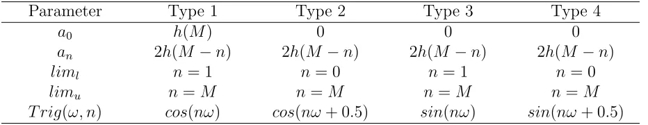
By introducing symmetry in the impulse response, a linear phase or constant group delay can be insured in an FIR filter. Based on the type of symmetry, four types of linear phase FIR filters can be categorized:
1. Type 1: The impulse response has odd number of coefficients (order of filter being even) and the coefficients are symmetric with respect to the midpoint.
2. Type 2: The impulse response has even number of coefficients (order of filter being odd) and the coefficients are symmetric with respect to the midpoint (not an actual point).
3. Type 3: The impulse response has odd number of coefficients (order of filter being even) and the coefficients are anti-symmetric with respect to the midpoint.
4. Type 4: The impulse response has even number of coefficients (order of filter being odd) and the coefficients are anti-symmetric with respect to the midpoint (not an actual point).
Due to the symmetry property of the linear phase FIR filters, their frequency response can be characterized by M + 1 unique coefficients,where M = bN−1
2 c for an N tap filter. Thus the amplitude response is given by Eq. 1.6
Ha(ω) = a0+
limu
X
liml
anT rig(nω) (1.6)
Table 1.1 shows the form of the amplitude response of linear phase FIR filters for each type of filter. The symmetric filters have a cosine term owing to the addition of the duplicate frequency response terms and the resulting cosine term due to the Euler’s formula. Anti-symmetric terms have a sine term due to the subtraction of the duplicate terms.
1.2
Filter Design Methodology and Specifications
Table 1.1: Amplitude Response of Linear Phase FIR Filters
Parameter Type 1 Type 2 Type 3 Type 4
a0 h(M) 0 0 0
an 2h(M −n) 2h(M−n) 2h(M −n) 2h(M −n)
liml n= 1 n = 0 n= 1 n= 0
limu n=M n =M n=M n=M
T rig(ω, n) cos(nω) cos(nω+ 0.5) sin(nω) sin(nω + 0.5)
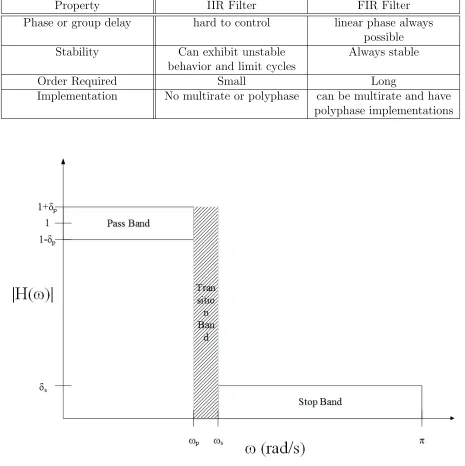
specified by a 4-tuple fspec (Fig. 1.1):
f spec= (ωp, ωs, δp, δs)
where ωp is the passband cutoff frequency, ωs is the stopband cutoff frequency, δp is the
maximum allowable passband ripple error andδsis the maximum allowable stopband ripple
error. The error specifications can either be given in decibels or in absolute error. The cutoff frequency can be either given in radians per second or in normalized form. The normalization is done either by diving by π or 2π. If the frequency is given in hertz, than the sampling frequency must also be given. In that case the 2π radians/s correspond to the sampling frequency and π radians/s to half the sampling frequency. Also, due to the sampling theorem, frequencies up to half the sampling frequency can be completely recovered in a sampled signal. Thus, if the specifications require higher frequencies than half the sampling frequency, the sampling frequency must be increased to ensure all the frequencies that are to be dealt with are less than half the sampling frequency.
Upon defining the specification, the filter order is estimated. The MATLAB function “f irpmord.m” gives a close approximation of the filter order. However, a few iterative designs have to be done till the specifications are met exactly and the filter order is not more than the minimum required for meeting the specifications.
Table 1.2: FIR vs. IIR
Property IIR Filter FIR Filter Phase or group delay hard to control linear phase always
possible Stability Can exhibit unstable
behavior and limit cycles
Always stable
Order Required Small Long
Implementation No multirate or polyphase can be multirate and have polyphase implementations
Table 1.3: Automatic Zeros of Linear Phase FIR Filters
Type Type 1 Type 2 Type 3 Type 4 Zeros None ω=π ω = 0, π ω = 0
The optimal filter design problem can be formulated in many ways depending on the objective function. Taking only the frequency into consideration and not the group delay the error can be defined as theLp norm (Eq. 1.7) of the weighted difference between the
amplitude response (Eq. 1.6) and the desired frequency response.
||x||p = ( n
X
i=1
|xi|p)1/p (1.7)
Thus, among the many possible Lp norms, the two cases that are most often used are
when p= 2 and p =∞. The Least Square design corresponds to p= 2 and its objective function is given in Eq. 1.8.
=
Z π
0
W(ω)|Ha(ω)−D(ω)|2dω (1.8)
whereW(ω) is given in Eq. 1.9 andD(ω) is given in Eq. 1.10 and Ωp,Ωs are the passband
and stopband frequency points respectively.
W(ω) =
Wp if ω ∈Ωp
Ws if ω ∈Ωs
0 otherwise
(1.9)
D(ω) =
1 if ω∈Ωp
0 if ω∈Ωs
any number otherwise
(1.10)
The least square design tries to minimize the energy difference between the desired response and the actual response.
is given by 1.11. As the L∞ norm corresponds to the maximum value of the vector,
the minimax design tries to reduce the maximum difference between the actual frequency response and the desired response (called ripple error).
=max [W(ω)|Ha(ω)−D(ω)|] (1.11)
For a detailed discussion of filter design techniques, the reader is referred to [1]. Also, the applications of digital filters and their implementation techniques are discussed in detail in [2].
1.3
Motivation and Outline of Thesis
Over the past decade portable electronic gadgets running on battery have become ubiqui-tous. Many new biomedical applications have emerged that require minimal power con-sumption. Thus, a new paradigm began in design of digital systems; one that accentuated low power design. This paradigm also made its way into digital filter design and recent researches have been focused on designing filters with low computational and hardware complexity.
The current finite word length filter design techniques that minimize hardware suffer from large design times or non optimal results. This thesis aims to develop a design algorithm that can generate a high level filter architecture such that the chip area, the computation cost and the power consumption are minimized. The proposed algorithm produces results competent with the best deterministic methods and also cuts down the run time of the algorithm.
The thesis is organized as follows. Chapter 2 gives the review of the literature present on the design of finite word length digital filters and hardware complexity reduction tech-niques. The techniques are broadly classified into multiplier less and with multipliers. The techniques with multipliers are briefly reviewed. The multiplier less techniques are reviewed in detail. The sum of power of two designs, the multiple constant multiplication algorithms and their application to filter synthesis and the state of the art techniques in minimal hardware filter designs are given.
Chapter 3 gives an overview of the optimization algorithms used throughout the the-sis. The choice of selecting an optimization technique based on the objective is firstly given. Next, the linear programming algorithm and its setup is given. Subsequently, the Differential Evolution algorithm is given in detail along with the variations in the muta-tion techniques, adaptive control parameters and the discrete variant of the Differential Evolution algorithm proposed in this thesis.
Chapter4gives the proposed algorithm for the design of minimal hardware complexity finite word length digital filters. The algorithm is referred to as Differential Evolution Filter Design Optimization (DEFDO) algorithm. The problem is formulated in section 4.1 and the DEFDO algorithm is given. Section4.2 gives a detailed mathematical and analytical discussion on the DEFDO algorithm. The various techniques employed at enhancing the run time and search of the Differential Evolution algorithm are also discussed.
and hardware complexity is carried out to show the working of the algorithm. Six filters from literature and two special filters have been implemented. An analysis of the filter orders and word length for implementation is given prior to the design examples. Section
Chapter 2
Review of Filter Complexity
Reduction Methods
Filtering operation is central to all digital signal processing systems. Design of optimal linear phase FIR filters has always been the focus of attention because of their marked superiority over IIR filters. The design that guaranteed optimality for infinite precision FIR filters was given by Parks-McClellan [3] which is to date the status quo in infinite precision techniques. However, with advances in communication, demands for filters with narrow transition width and high stopband attenuation requiring large orders prompted researchers to develop hardware reduction techniques. This chapter will first give an overview of the filter complexity reduction techniques. The multiplier less techniques will be discussed in detail. A brief overview of techniques that utilize multipliers such as sparse filter designs and frequency response masking approach would also be given.
2.1
Filter Complexity Reduction Technique
coefficients, the other techniques involve cascading filters and other circuitry to reduce the hardware complexity. However, for single stage filters, multiplier-less filters have proven to be very effective.
1. Complexity Reduction with Multipliers
• Recursive running-sum prefilters
• Cyclotomic polynomial prefilters
• Interpolated FIR filters
• Frequency-response masking technique
• Multirate techniques
• Multi-Stage decomposition
• Sparse filter techniques
2. Multiplierless Filter Design
The most researched upon techniques in designs utilizing multipliers are sparse designs and frequency response masking technique designs. They are briefly discussed here and further information on these design techniques can be found in the references.
Sparse Filter Design
Sparse filter design techniques aim at minimizing the non-zero coefficients in a digital filter. A zero coefficient implies no computation cost and thus maximizing the number of zero coefficients or minimizing the number of non-zero coefficients reduce the computational complexity of the digital filter.
A sparse filter design is anl0 minimization problem (Eq. 2.1).
subject to: |H(ω)−D(ω)| ≤∆(ω), ∀ω ∈ΩI
where x is the vector containing the unique filter coefficients, ∆(ω) is the tolerance in the frequency response andD(ω) is the desired frequency response, ΩI is the set bands of
interest in frequency and H(ω) is the amplitude response of the filter.
Among the notable methods for sparse filter design are linear program techniques given in [4] and a WLS relaxation approach is given in [5].
Frequency Response Masking
Lim, [6], introduced the frequency response masking technique for designing filters that had a narrow transition width. Because of sharp frequency characteristics, a single stage design required a huge number of taps for complying with commendable error constraints. In sparse filter design, the filter with is wide transition width is upsampled by replacing the delay element byM delay elements. Thus, the frequency response is a periodic and shrunk version of the initial frequency response curve. The ratio that the frequency response is shrunk by and the number of replicas that are generated depends on the factor M. Subsequently, a mask filter whose transition width is much larger is cascaded to filter out the unwanted replicas of the upscaled filter. Hence, a filter with a transition width of ∆/M is obtained where ∆ was the original transition width. Even though the mask involves extra hardware, however, compared to the hardware needed to design the narrow transition width filter on its own there is a substantial saving in the hardware. For a detailed discussion of frequency response masking the reader is reffered to [6] and [7].
2.2
Multiplierless Filter Design
loss in accuracy takes place in going from infinite precision to finite precision by simple quantization to the nearest value. However, it was noted that the loss in accuracy can be mitigated to a great extent by formulating the optimization problem that took into account the discrete nature of the filter coefficients. Initially, two classes of optimization problems that handled finite word length filters emerged: exact and approximate [8]. The exact methods were based on search techniques that encompassed the entire space while the approximate techniques utilized local search algorithm in the neighborhood of continuous coefficients.
Many design techniques have evolved over time for designing discrete coefficient filters. Among the most notable ones are the signed power of two (referred to as SPT, SOPOT or POT), the Multiple Constant Multiplication and dynamically expanding subexpres-sion space design techniques. The following sections discuss each of the following design techniques and review their strengths and weaknesses.
2.2.1
Design of Discrete Filters in Sum of Power of Two Space
Design of discrete filters was first proposed by Kodek, [9]. He utilized a integer program-ming package and upscaled the coefficients to fit into the integer subspace. The branch and bound technique was proven to be successful in designing the discrete coefficient filter. However, the gains in the error as compared to the simply quantized optimal infinite preci-sion designs were not substantial. Thus, the amount of time required for design outweighed the gain in the error.
To justify such long design times Lim et al, [10] proposed the design of the discrete filter in the power of two subspace. Since a power of two did not require any hardware for its implementation as it could be generated simply by hardwired shifts, the substantial reduction in hardware complexity proved very attractive. In Lim’s design each coefficient was represented as a sum of two powers of two (Eq. 2.2).
h(n) =
L
X
i=1
where L = 2, Si(n) ∈ −1,0,+1 and −9 ≤ gi(n) ≤ 0. The method was suitable for
designing filter of length upto 40 using the computing resources available at that time. The paper paved the way for future research in discrete filter optimal designs.
In [11], the filter design objective was modified to the Normalized Peak Ripple Mag-nitude. This was owed to the fact that a filter’s purpose is to alter an incoming signal to allow one set of frequencies while attenuating another set of frequencies. Thus, a gain of unity was inconsequential. However, a constraint had to be set on the passband gain. A high gain meant a better signal to noise ratio but it also caused overflow. In the discrete power of two space, the upper bound and lower bound of the passband gain differed by two i.e. the lower bound was always half the upper bound. This was because any other gain could always be represented in the given range by multiplying or diving by a suitable power of two and the NPRM would remain the same. To find a coefficient set with the op-timal NPRM, passband gain sectioning was introduced. In the gain sectioning technique, the gain range was divided into many fine gain sections and a discrete filter was designed using the upper bound and lower bound constraints of the section on the gain. A simple technique was to section the range [0.7,1.4] and select the best solution found among all the sections. A trade off was met between design quality and design time as more sections led to a better design but with increased design time. A more involved technique based on elimination was also given.
Figure 2.1: Transposed Direct Form
a mild affect on the hardware complexity. Also, since impulse responses of low pass filters exhibit asinx/xsort of response, the percentage of large coefficients was small. The design algorithm first determined the scaling factor and then ran a local bivariate neighborhood search around the scaled and rounded coefficients.
In [13], a SPT term allocation scheme was developed where each coefficient is allotted different number of SPT terms based on its sensitivity to the frequency response. After assigining the SPT terms, an integer-programming algorithm was used to optimize the coefficient values. This new technique produced designs that had a much better NPRM as more emphasis was laid on coefficients with larger magnitudes.
2.2.2
MCM Algorithms
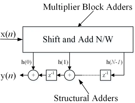
Figure 2.2: Shift and Add Network
the partial results generated could be utilized for multiple coefficients generation. This work paved the way for further research in Multiple Constant Multiplication algorithms as a means for implementing filtering and other DSP transforms.
y(i) =h(i)x i= 0,1· · ·N (2.3)
In defining the fixed coefficient filtering operation as a Multiple Constant Multiplication problem, the multipliers in the transposed direct form filter structure are replaced by a Shift and Add Network (SAN). The adders used for implementing the coefficients inside the SAN are referred to as Multiplier Block Adders (MBAs). The adders summing the delayed and weighted input are referred to as Structural Adders (SA). The MCM optimization problem has been widely researched and is proved to be NP-complete problem justifying the use of heuristic algorithms for solving the problem [15]. Figure 2.3 shows the comparison of the three approaches to implementing the filter coefficients.
(a) Multiplier Approach (b) SOPT Approach (c) MCM Approach
Figure 2.3: Filter Design Approach
Elimination algorithms first define the constants to be multiplied in a number represen-tation e.g. Binary, CSD, or Minimal Signed Digit. After that the common subexpression present in the numbers are obtained. The most common subexpression is used for sharing among the coefficients. The graph based technique do not utilize any specific number rep-resentation and represent the adder network as a graph and construct child tree branches from the parent branches. The RAG-n algorithm [18] is the most notable graph based algorithm. It consists of 2 parts: exact and heuristic. The exact part of the algorithm outperforms all CSE algorithms, however its applicability to a given set of numbers is re-stricted. It can only synthesize constants that can be represented as a sum of two other coefficients using one adder and there exists at least one constant which is a cost one constant [19]. The CSE algorithms have the disadvantage that they are specific to a num-ber representation and only search the common subexpression space. The filter design technique proposed in this thesis utilizes the exact part of RAG-n algorithm and is thus explained in detail.
Reduced Adder Graph-n Algorithm
Definition: Adder Cost
The adder cost of a set of constant integers is the number of adders and subtracters required to perform multiplication by all those constants.
Definition: Fundamentals
The intermediate or final odd values (the vertices of the graph) used in synthesizing the shift and add network.
The RAG-n algorithm utilizes the lookup tables generated by the MAG algorithm [19]. One lookup table gives the adder cost of multiplying by an integer and the other lookup table gives the different set of fundamentals that can be used to implement the constant multiplication optimally. The steps of the algorithm are enumerated for generating a shift and add network of constants with word lengthB:
1. Obtain the odd fundamentals from the set by taking the odd numbers and diving even numbers until an odd number results and delete the repeated numbers. Call the set “incomplete set”
2. Find among the “incomplete set”, cost one fundamentals form the lookup table.
3. Add the cost one fundamentals to the “graph set” and remove them from the “ in-complete set”.
4. Examine pairwise sums of the form (a×2i±1) or (a×2i±b) wherea, b∈“incomplete set”
andiis an index that is varied from 0,1,· · ·B. If any coefficient from the “incomplete set” is found, remove it from the “incomplete set” set and add it to the “graph set”. 5. Repeat until no more coefficients remain in the “incomplete set”.
The enumeration gives the exact part of the RAG-n algorithm. The following theorem were proved in the paper and also provide useful insight into applicability of the exact part of the algorithm:
Theorem 2: For a set to incur the minimal adder cost ofn, at least one cost-1 coefficient must be in the set.
The exact part of the algorithm may not always synthesize and a supplemental heuristic algorithm is given in the paper. However, since in this thesis only the exact part is utilized, the heuristic part is not explained.
2.2.3
State of the Art
The MCM problem was limited in the sense that it only optimized the already synthesized coefficients. However, a coefficient set complying with a particular design constraint is not unique. Thus, a coefficient set which in the representation sense was not minimal could possibly have a better hardware implementation than the one with the minimal bit repre-sentation. This problem was circumvented by including the synthesis of the shift and add network in the optimization of the discrete coefficient representation. The latest research in multiplierless design is focused on cutting the design time while maintain optimum perfor-mance level. Since the exact techniques, which employ mixed integer linear programming (MILP) branch and bound or tree search algorithms such as width recursive depth first search, have exponential growth in complexity with the filter order thus they cannot be used for designing higher order filters without proper pruning techniques.
A few new terms were defined in [20] for the discrete filter design problem. The concept of bases or fundamentals was already in use in MCM designs, but [20] extended the defini-tion to include subexpression space. The definidefini-tions are repeated here and used throughout the thesis.
Definition: Basis Set
In the synthesis of the SAN, the intermediate or final odd values are called fundamentals or bases. The set of all the bases needed to synthesize the SAN is the basis set.
Definition: Subexpression Space
subexpression space is defined as
n=
T−1
X
i=0
si2mi (2.4)
wheremi is a non-negative integer andsi ∈S and S is the basis set. For the SOPT space,
the basis set isS ={−1,1}. Other examples of basis set are S1 ={0,±1,±3,±5}. Definition: Contiguous Basis Set
A basis set if said to be contiguous if it contains all contiguous odd integers till the largest odd integer present.
Definition: Order of Basis Set
The order of a basis set is defined as the number of adders required to construct the basis set.
Branch and Bound MILP
The linear phase FIR filter design problem for continuous coefficients can be modeled as a linear program. Thus, it can be solved easily using polynomial time algorithms for linear programming. However, if the coefficients are forced to take discrete values than the problem becomes NP-complete. By upscaling the coefficients, the problem can be modeled as a Mixed Integer Linear Program. To tackle the problem, a linear relaxation approach is developed whereby the discrete constraint is dropped and the problem is solved as a linear program. However, simply quantizing the solution of the relaxed problem can result in the solution lying very far away from the optimal discrete solution. Thus, a branch and bound technique is developed to systematically solve relaxed linear programs and further branches are created or fathomed depending on the feasibility of the solution of the relaxed problem.
The branch and bound MILP is used in [20] to find the optimal coefficients from a fixed subexpression space. An upper cap on the number of adders is obtained and the frequency response ripple is minimized. Firstly, a continuous solution is obtained using linear programming. Among the coefficients a coefficient, sayxi, is selected for branching.
the following bounds on xi are xi ≥ 6 and xi ≤ 5 respectively. The depth first search
progresses by keeping L2 aside and exploring L1 further. Another coefficient, say xj, is
chosen and the bounds ofxj ≥ dxje and xj ≤ bxjcare imposed giving rise to subproblems
L3 and L4. L4 is kept aside and L3 is further explored. The process continues till all the coefficients have been fixed and a discrete solution is obtained. Thus that branch is terminated and the algorithm back traces to solve the adjacent problem. A node is also terminated if it is seen that an optimal solution is not possible upon further exploration.
The algorithm suffered from the following problems:
1. Prefixing the Basis Set: The set of numbers and the space to search for the optimal filter coefficients was fixed apriory. Thus, the choice limited the search space and hence the optimal solution. A lot of effort had to be made to define a basis set that would best serve the problem at hand.
2. Determining the closest approximation: The closest number that can be represented in the subexpression space to serve as the bounds of the linear program was to be determined. An exhaustive search or a greedy algorithm was utilized which slowed down the process. A lookup table could be generated for static subexpression spaces which cut short the time consumed in the search process.
3. Tradeoff Between Order of Basis Set and Number of Terms Per Coefficient: A trade-off had to be met whereby choosing a small order basis set meant using more number of terms to construct a coefficient or choosing a large order basis set and using less number of bases for constructing the coefficients.
Dynamically Expanding Subexpression Space Design
The optimality of the basis set can be obtained by dynamically expanding the basis set based upon the need for discretizing the coefficients starting from the trivial basis set 0,±1. In this method, the coefficients that are likely to result from the usage of less adders are discretized first. However, for solving the problem in a dynamically expanding subexpression space, the branch and bound MILP cannot be used and hence in[21], [22], [23] MILP with depth first width recursive search is used. In this method, a coefficient is selected for discretization and it is branched to L different branches with the L closest discrete values selected in each branch. With one coefficient fixed, the rest of the coefficients are again optimized and another coefficient is selected for discretization. Again, a set of L branches are formed. In the depth first search, only one among the L branches at each stage is selected for further branching. When, all the coefficients have been discretized, then the solution is stored and the algorithm back traces and solves the other branches at the next upper level. Also, for expediting the search process, the solution of a branch is compared with the current best obtained solution and if it cannot offer a better solution, it is not further explored.
The complexity of the above algorithm depends highly on the number of braches (L) that are created at each stage. In [21],Lbranches are created such that only one adder must be used in the synthesis of the discrete value from the already existing subexpression space and theseLvalues are the closest to the continuous coefficient value. In [22], an exhaustive search is made where all the possible discrete values are selected for branching based upon a feasible range of that coefficients (calculated beforehand). Thus, the complexity of the depth first width recursive search is exponential with L.
needed to synthesize the smaller group of coefficient.
Genetic Algorithm Based Filter Design
The paper [25] uses a genetic algorithm for designing the multiplier-less filter. In their algorithm, a reduced search space is created around a base solution. The base solution is obtained by discretizing a continuous solution for a corresponding gain. Also, they have encoded the difference between the possible values the GA can take to the base solution as the value the chromosomes of the GA represent leading to a shorter encoding scheme. Thus, they have managed to reduce the search space and expedite the search process of the GA. Also, the mutation and crossover operations have been modified and the rates made adaptive.
The number of adders in the implementation has been set as the objective to minimize. They make use of the RAG-n [18] algorithm for determining the number of adders. Since for each passband gain the search process is independent, they have cast each problem to a different machine and ran in parallel. However, since the RAG-n algorithm consumes a substantial time, they formulate a fitness function that inhibits the algorithm for running the RAG-n algorithm for solutions that do not meet the error constraints. For a filter order of 324, their design time is around 3h49m when casted onto 20 machines or 37h9m when completed on a single machine.
Summary
Chapter 3
Optimization Methods
Optimization is the process of minimizing the cost or maximizing the gain of a process or function. Optimization is performed in every field from economics to engineering. The technique to approach a particular type of problem depends on the characteristics of the problem whether the function is linear or nonlinear, convex or non-convex, constrained or unconstrained. Also, a function maybe multi-objective where a number of objectives need to be optimized simultaneously or multimodal where multiple equally good solutions exists. The problem may be defined on the set of real number whereby the parameters are continuous, or on a discrete set of number where the parameters take discrete values or the problem may be mixed where some parameters can take continuous values while others can only take discrete values.
examined.
3.1
Selection of Optimization Method
The theory of continuous parameter optimization has been developed for centuries and is at present very mature. Efficient algorithms exist for linear problems with linear inequality and equality constraints. Quadratic unconstrained problems can be solved using gradient based methods such Quasi Newton algorithm. A detailed discussion on optimization can be found in [26].
While continuous parameter optimization is tractable however, situations arise when the parameters can take values only from a finite set. If the finite set is the set of integers, the problem is modeled as integer programming or if they belong to a mixed set consisting of real numbers and integers then mixed integer programming models are used provided the constraints are linear. However, if the constraints follow no general rule then the problem is generally classified as a combinatorial optimization problem. In this problem, the possible solution is a combination from a finite set of points with the objective function and the constraints taking any form. The problems in combinatorial optimization are ranked based on the computational complexity.
Definition: Computational Complexity of Algorithms
The complexity of an algorithm to solve a given problem is generally specified by the worst case scenario. TheO notation is used to denote the complexity which is defined as
f(n) = O(g(n)) (3.1)
if there exist positive constants a and b such that ∀n > a, f(n)≤b.g(n)
O(bn),b > 1. Problems for which polynomial time algorithms exist for solving them are
called tractable and if a polynomial time algorithm does not exist than they are intractable. Two classes of algorithms exist for solving combinatorial optimization problems :
1. Exact Algorithms
2. Approximate Algorithms
The exact methods include branch and bound algorithms, graph based tree search (breadth first or depth first) while approximate methods include approximation algorithms, heuristics and metaheuristics. The choice of algorithm for approaching a certain problem is dependent on whether it is a P problem or not. AP problem is a problem for which a polynomial time algorithm exists for solving it. AnN P problem is one whose solution can be verified in polynomial time. AN P −Hard is problem which is as hard as the hardest N P problem. N P −Hard problems which are also N P are known as N P −Complete problems. Deterministic algorithms should be used if the problem isP and use of heuristics is unjustified. Also for N P −Complete problems, the instance of the problem must be considered as small instances can solved easily by exact algorithms. The justifiable use of heuristics is in large instances of N P −Complete problems. If, however, the polynomial time algorithm has high order index than use of heuristics might be favored.
3.2
Linear Programming
Linear Programming is a method for optimizing a linear functions subject to linear equali-ties and inequaliequali-ties. The generalized linear programming problem can be defined as: Find x∈RN such that the function
f unc(x) =fTx=
N
X
i=1 fixi
a11x1+a12x1· · ·+a1NxN ≤b1 a21x1+a22x1· · ·+a2NxN ≤b2
.. .
aM1x1+aM2x1· · ·+aM NxN ≤bM
and P equality constraints
c11x1+c11x1· · ·+c1NxN ≤d1
c21x1+c22x1· · ·+c2NxN ≤d2 ..
.
cP1x1 +cP2x1· · ·+cP NxN ≤dP
and the following bounds on the variables
x1l ≤x1 ≤x1u
x2l ≤x2 ≤x2u
.. .
xN l ≤xN ≤xN u
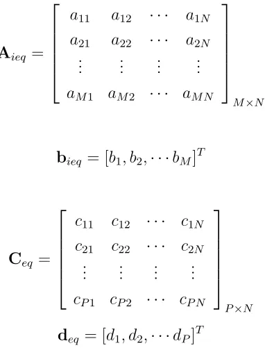
Table 3.1: Linear Program Setup min fTx
Aieqx≤bieq Inequality Constraint
Ceqx=deq Equality Constraint
xl ≤x≤xieq Bounds on Variables
Rewriting the constraints in matrix form
Aieq =
a11 a12 · · · a1N
a21 a22 · · · a2N
..
. ... ... ... aM1 aM2 · · · aM N
M×N
bieq = [b1, b2,· · ·bM]T
Ceq =
c11 c12 · · · c1N
c21 c22 · · · c2N
..
. ... ... ... cP1 cP2 · · · cP N
P×N
deq = [d1, d2,· · ·dP]T
or outside the feasibility polyhedron. Many authors have proposed techniques for solving problems.
The OPTI Toolbox, [27] is an open source collection of optimization algorithms made available. The CSDP Algorithm by Borchers, [28], is utilized in this thesis for solving filter design problems.
3.3
Differential Evolution Algorithm for Continuous
Optimization
Among the class of global optimization algorithms, Evolutionary Algorithms (EA) are metaheuristic algorithms. The strategies employed in EAs are inspired by biological phe-nomenon of evolution and survival of the fittest. Among the notable techniques are Ge-netic Algorithm (GA) and Differential Evolution (DE). EAs create a random population of parameter vectors in the search space representing all the landscape. The population members interact with each other through operators such as crossover, mutation, and new generations are produced using selection. Closely related to EAs are algorithms utilizing swarm intelligence e.g. Particle Swarm Optimization (PSO), Ant Colony Optimization (ACO) etc.
Given an objective function with Dparameters to be optimized. The Differential Evo-lution algorithm begins by creating a population ofNp D-dimensional random vectors. The
simple DE employs three operators to evolve from one generation to the other: mutation, crossover and selection (Figure3.1).
Initialization
Figure 3.1: Pseudo Code for the Differential Evolution Algorithm process DE
1 initialization
2 do
3 mutation 4 crossover 5 selection
6 while (termination criteria) end process
and bl respectively, then the values are generated according to Eq. (3.2).
xp,j1 =bl,j+rj(bu,j −bl,j) (3.2)
where rj ∈ (0,1) is a random number and j = 1,2, D. The first generation (g = 1)
population is created by repeating the above process Np times. Let each member of the
population be represented as in Eq. (3.3).
xp,g = [xp,g1 , xp,g2 , ...xp,gD ] (3.3)
where p = 1,2,→ Np and g = 1,2, gmax. Subsequently, the population can be
repre-sented as a NpD matrix (Eq. (3.4)).
Pg = [x1,g, x2,g, ...xNp,g]T (3.4)
Mutation
The mutation operator produces a population of trial vectors. For each member of the population, called target vector of index p, the trial vector up,g+1 is generated using Eq. (3.5).
The indices r1, r2, r3 are all distinct and also different from the target index p. F ∈
(0,1) is a scaling factor and is one of the control parameters.
Crossover
The crossover operator combines parameters from the target vectorxp,g and the trial vector up,g+1 to generate the mutant vector yp,g+1. The parameters of the mutant are selected according to Eq. (3.6).
yjp,g+1 =
(
up,gj +1 if r ≤CR orj =jrand
xp,gj if r > CR (3.6)
forj = 1,2, D and r∈(0,1) is a random number andjrand is a randomly selected integer between 1 and D (both including). CR ∈[0,1] is the crossover probability and it reflects the amount of information that is inherited from the trial population. A random number index, jrand, is also checked for to ensure that the target vector is not replicated.
Selection
The selection operator is responsible for creating new generation from among the trial vectors. For each target vector, if the objective function value is less corresponding to the mutant vector, then the mutant vector replaces the target vector in the population. Thus, selection can be done according to Eq. (3.7).
xp,g+1 =
(
xp,g if f(xp,g)≤f(yp,g+1)
yp,g+1 otherwise (3.7)
3.4
Variations of Differential Evolution
3.4.1
Variation in Mutation
The DE algorithm described in section 3.3 is the most basic form. It is denoted as
DE/rand/1/binas the base vectorxr1,g in Eq. 3.5is randomly chosen and there is only one
differential term F.(xr2,g−xr3,g) and the mutation operator exhibits a binomial
distribu-tion. There is another form of mutation called exponential but for brevity its definition is omitted. Storm and Price, [29], have also given other variations which are described below. They all differ in how the mutation operator takes place. Thus, the mutation equation for each is given.
1. DE/best/1/bin
up,g+1 =xbest,g +F.(xr2,g−xr1,g) (3.8)
2. DE/best/2/bin
up,g+1 =xbest,g +F.(xr2,g−xr1,g) +F.(xr4,g−xr3,g) (3.9)
3. DE/rand/2/bin
up,g+1 =xr1,g+F.(xr2,g−xr3,g) +F.(xr4,g−xr5,g) (3.10)
4. DE/tar2best/1/bin
up,g+1 =xi,g+F.(xbest,g −xi,g) +F.(xr2,g−xr1,g) (3.11)
3.4.2
Adaptive Control Parameters
solution, it does not influence the convergence of the algorithm. The other two parameters influence the convergence and must be properly set with trial and error. Brest et al, [30], have proposed an adaptive control parameter adjustment technique. With slight modifi-cations to their results, equations 3.12 and 3.13 are obtained to be used in the discrete DE.
Fp,g+1 =
(
Fl+r1∗(Fu−Fl) if r2 < τ1
Fp,g otherwise (3.12)
CRp,g+1 =
(
CRl+r3∗(CRu−CRl) if r4 < τ2
CRp,g otherwise (3.13)
wherer1, r2, r3, r4 ∈(0,1) are random numbers,τ1 =τ2 = 0.1 and Fl, Fu and CRl, CRu
are the lower and upper bounds of F and CR. The values used are Fl = 0.4, Fu = 1,
CRl= 0.05 andCRu = 0.2.
3.5
Differential Evolution for Discrete Filter
Optimiza-tion
The original Differential Evolution algorithm is used for real valued parameter optimiza-tion. Due to its superior convergence characteristics, researchers have attempted to utilize the differential approach for discrete parameter optimizations. Strategies based on trunca-tion of the parameters for calculating the objective functrunca-tion value were proposed initially. Other techniques involved defining the population member as a permutation of numbers. However, the essence of the DE being the differential operator for mutation was not fol-lowed in these methods.
four operators defined on the sets. In the crossover, the learn procedure is utilized whereby the trial learns either from the target or the trial vector to obtain the mutant vector. In both the papers a complex representation of the parameters for population generation and evolution is given. Also, the concept of Hamiltonian circuit constraint satisfiability further accentuates the complexity. However, such complex representation is not needed for the filter design problem as each parameter can have only a single value and is selected from a discrete set.
A new discrete Differential Evolution algorithm inspired by the set based algorithms is proposed for the finite word length filter design. The algorithm utilizes a bit string and integer population and a decode scheme is implemented for converting the one from the other. Consider a function f(x) defined over the vector x = [x1, x2...xD]T ∈ ZD where
D is the number of parameters to be optimized and Z is the set of integers. This form of the vector is employed in this thesis as the filter coefficients have been scaled up by multiplying with a suitable power of two such that they can be represented as integers. So, the minimization of the function is carried out in the integer subspace and each parameter represents the unfixed filter coefficient.
To find the optimal discrete value of the filter coefficients, the mutation, crossover and selection operators of the Differential Evolution are applied. For the crossover and selection operators the equations given in section3.3 (Eq. 3.6,3.7) can be applied directly and the resulting output would lie in the integer subspace. However, the mutation equation (Eq. 3.5) will yield a result that lies outside the integer subspace. Thus, for the mutation operator, each parameter is encoded into a bit string consisting of a total of N bits for the D parameters. The actual encoding and bit allocation scheme is implemented taking into account the problem to be solved. For the finite word length filter design problem it is discussed later with the proposed algorithm. To summarize the scheme, the mutation operation is performed on the N bits and is explained in the following paragraphs. The crossover operation is performed on the D parameters and is the same as discussed in section3.3.
To obtain the trial vectors Eq. 3.5 is redefined and each of the N bit position (bi) is
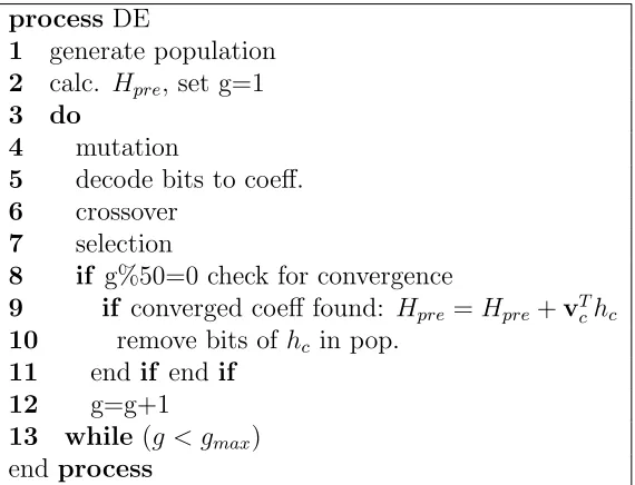
Figure 3.2: Pseudo Code for Discrete Differential Evolution process discrete DE
1 generate population of P members∈Z with D parameters 2 encode each D parameter as a bit string
3 g=0 4 do {
5 for i= 1 :P 6 for j = 1 :N 7 mutation 8 end for
9 decode from bit to integer 10 for j = 1 :D
11 crossover 12 end for 13 for j = 1 :D 14 selection 15 end for 16 end for 17 g=g+1 }
18 while (g < gmax)
output: best solution end process
bdi =
(
bxir2 if bxir3 = 0
0 if bxir3 = 1 (3.14)
bF.i d =
(
bd
i if rand(0,1)< F
0 otherwise (3.15)
bui =
(
1 if bxr1
i = 1
bF.d
i otherwise
(3.16)
where i= 1,2, ...N and rand(0,1)∈(0,1) is a random number.
al-gorithm. The algorithm is utilized along with adaptive control parameters (section 3.4.2) for designing finite word length filters (Chapter 4). The discrete Differential Evolution algorithm presented can also be used for optimizing functions where the coefficients are independent of each other and belong to the set of integers.
Summary
Chapter 4
Proposed Algorithm
Chapter 2discussed the various techniques for reducing the hardware complexity of finite word length digital filters. Among the multiplierless techniques, the sum of power of two design was successful in reducing the hardware complexity. However, large orders were needed to meet stringent error constraints. The multiple constant multiplication algorithms gave a new approach and focused on reducing the redundancy among the coefficients to reduce the hardware complexity. However, the MCM did not take into account the design procedure of the filter coefficients. The latest techniques jointly find the filter coefficients and reduce the hardware. However, among the state of the art algorithms present, the deterministic MILP based algorithms have an exponential computational complexity. The heuristic methods are fast but give out inferior designs.
4.1
Problem Formulation
In this section, the proposed filter design method is discussed. The proposed technique in-volves a combination of linear programming and evolutionary algorithm. The evolutionary method is a hybrid Differential Evolution method discussed in Chapter3 in sections 3.4.2
and 3.5. The adaptive control parameters have been used and for the mutation operator, a bit string method described in section3.5 is implemented.
4.1.1
Minimax Error and Adder Cost Joint Objective Function
Calculation
For the discrete filter design problem, the problem can be divided into two parts: subject and object (as refereed to in [33]). The object is the main aim of the problem i.e. minimize the hardware complexity while the subject are the constraints that have to be satisfied i.e. the maximum allowable ripple error. Hence, the optimization problem can be modeled as in Eq. 4.1.
minimize
M
X
i=0
Cost(xi) (4.1)
subject to:
∆≤δp (4.2)
where x is defined as the vector x = [x0, x1...xM]T ∈ ZM+1, ∆ is the weighted minimax
error (Eq. 4.3) and δp is the maximum allowable error in the passband as defined in the
filter specifications (fspec). The values of vector x are related to the filter coefficients as hn = xM−n+1 = hN−n−1. The passband error (δp) is considered for comparison as the
weight of the pass band is fixed to be unity.
∆ = max[W(ω)|Ha(ω)
whereHa(ω) is the amplitude response of the filter, D(ω) is the desired function,W(ω) is
the weighting function and G is the passband gain. Eq. 4.4 and 4.5 give the expressions for the weighting function W(ω) and the desired function D(ω). The value of passband gain Gis given by (4.6).
W(ω) =
1 if ω ∈Ωp δp
δs if ω ∈Ωs
0 otherwise
(4.4)
D(ω) =
1 if ω∈Ωp
0 if ω∈Ωs
any number otherwise
(4.5)
G=
( Gp,max+Gp,min
2 if
Gp,max−Gp,min
2 >
δp
δsGs,max
Gp,min+ δp
δsGs,max if otherwise
(4.6)
where
Gp,max =max|Ha(ω)|ω∈Ωp
Gp,min =min|Ha(ω)|ω∈Ωp
Gs,max=max|Ha(ω)|ω∈Ωs
In Eqs. 4.4, 4.5, 4.6 Ωp is the set of frequencies belonging to the pass band, Ωs is the set
of frequencies belonging to the stop band.
Since in Eq. 4.3, the coefficients are represented in the integer subspace and Normalized Peak Ripple Magnitude is used, hence the amplitude response is divided by the passband gain, given by Eq. 4.6, in order to determine the error constraints which are given for unity passband gain. Eq. 4.7 shows the expression for the amplitude response of a linear phase filter.
Ha(ω) = vTcx (4.7)
on the type of filter. Eq. 4.8 gives the expression for Type I and Type II filters for vc.
Similar expressions can be derived for Type III and Type IV filters.
vc=
(
[1,2cos(ω), ...2cos((M −1)ω),2cos(M ω)]T for Type I
2cos(0.5),2cos(ω+ 0.5)· · ·2cos((M −1)ω+ 0.5),2cos(M ω+ 0.5) for Type II (4.8)
4.1.2
The Differential Evolution Filter Design Optimization
Al-gorithm
In the previous section (4.1.1), the objective of the problem was defined along with the constraints. In this section an algorithm that achieves the objective is given. The algorithm if referred to as Differential Evolution Filter Design Optimization (DEFDO). The method is summarized below and explained in detail in the next section.
1. The index of the coefficients that can be made zero, denoted asZ, is found first. For small to medium length filters, Z is found by finding the range using Eq. 4.9.
minimize f =h(k) f =−h(k) (4.9)
for k = 0,1...bN−1 2 c
subject to: (1−δp)≤Ha(ω)≤(1 +δp) for ω∈Ωp −δs ≤Ha(ω)≤δs for ω ∈Ωs
where
Ha(ω) = bN−1
2 c
X
n=0
T rig(ω, n) is the trigonometric function based on the type of FIR filter for an N tap filter. Those coefficients whose range includes the zero crossing are possible candidates forZ. The optimal infinite precision coefficients are found by solving the linear program in Eq. 4.10 and setting Z =φ.
minimize f =δ (4.10)
subject to: (1−δ)≤Ha(ω)≤(1 +δ) for ω ∈Ωp −δδp
δs
≤Ha(ω)≤δ
δp
δs
for ω ∈Ωs
Ha(ω) = bN−1
2 c
X
n=0,n /∈Z
h(n)T rig(ω, n)
The coefficient, among the Z candidates, whose absolute value is the least is fixed as zero and the linear program is again solved to find the minimax error (δ). The process iterates by including the next candidate until the minimax error exceeds the required error. Sometimes, it is needed to back trace the steps and include lesser zeros in the coefficients than given by the algorithm in order to accommodate the loss in precision due to quantization of the coefficients. The last optimal coefficient values are denoted by the vector hc. The range is again calculated by fixing the
zero coefficients. Let the range of each unique coefficient be denoted by [ri
l, rui] for
i = 0,1· · ·M. The expanded form and explanation of the linear programs is given in section 4.2.1.
2. For a given effective word length (EW L), it is needed that the greatest coefficient can be represented in the specified number of bits. So, if the coefficient set hc has a
gain of 1, then the maximum gain whose greatest coefficient can take a value up to 2EW L−1 is given by Gu, where Gu is defined as
Gu = 2
EW L−1 khck∞
Table 4.1: Range of Filter Lower Limit (ri
l) Optimized Coefficient (hc) Upper Limit (riu)
0.3138 0.3300 0.3457
0.1964 0.2012 0.2051
0.0279 0.0430 0.0581
-0.0556 -0.0439 -0.0342
-0.0487 -0.0427 -0.0369
-0.0174 -0.0070 0.0026
0.0059 0.0124 0.0195
0.0020 0.0091 0.0147
Gl= G
u
2 (4.12)
The gain range, [Gl, Gu], is divided into S equally spaced sections. For each section
the lower range is denoted asgs,l and the upper range is denoted asgs,u. The number
S is taken according to the hardware capability and the time constraint of the design procedure. Thus, a trade-off is met between design time and design accuracy.
3. The optimization problem is solved by generating a population as explained in section
4.2.2 in the gain range and running a local search using the Differential Evolution al-gorithm described in Chapter 3. The variant of the DE used isDE/rand/1/bin along with adaptive control parameters. The algorithm also utilizes adaptive search space reduction (section 4.2.5) and the selection operator given in section4.2.4. Techniques used for shortening the run time are also used (section 4.2.6). The synthesis of the SAN is carried out by modifying the RAG-n algorithm (section 4.2.3).
EW L = 7 design shown in Chapter 5 this coefficient has been fixed to zero. However, forEW L = 6, fixing this coefficient to zero renders the filter search space not to give out feasible solutions.
4.2
Algorithms Used In DEFDO
In this section, the DEFDO algorithm and adjustments in the Differential Evolution al-gorithm tailored for the filter design problem are discussed. Firstly, the linear programs used in section4.1 are explained in detail. Next, the population generation mechanism for the DE algorithm is explained. After that the modified version of the RAG-n algorithm which gives the hardware cost is explained. Subsequently, the selection operator of the DE algorithm is explained. Lastly, enhancements for the DE algorithm are discussed which include adaptive sub space reduction. Next, methods to cut short the computation time are discussed. Lastly, the modified RAG-n algorithm for the synthesis of filters is given.
4.2.1
Linear Programs Used in Filter Design
The linear programs of Eqs. 4.9 and4.10are solved on a dense grid on frequencies in [0, π]. Let the frequency grid be represented as Ω = [ω1, ω2, ...ωn] and the filter coefficients as
hf = [h0, h1,· · ·hN−1] for an N tap filter. Also let M =bN2−1c. The inequality
W(ω)|Ha(ω)−D(ω)| ≤δ
can be written as
Ha(ω)−
δ
W(ω) ≤D(ω)
−Ha(ω)−
δ
whereW(ω) and D(ω) are defined in Eqs. 4.4, 4.5 respectively. Since the linear program is evaluated on Ω, the above inequalities are written as
h−wδ≤d
−h−wδ≤ −d
where
h= [H(ω1), H(ω2),· · ·H(ωn)]T
w= [1/W(ω1),1/W(ω2),· · ·1/W(ωn)]T
d= [D(ω1), D(ω2),· · ·D(ωn)]T
The vectorh can be written as
h=Cg where C is defined for Type I filter as
C=
1 2cos(ω1) · · · 2cos(M ω1) 1 2cos(ω2) · · · 2cos(M ω1)
..
. ... ... ... 1 2cos(ωn) · · · 2cos(M ωn)
g= [hM, hM−1,· · ·h0]T
in Eq. 4.13.
x=g f= [0,0,· · · ±1,· · ·0]TM+1×1
Aieq =
"
C
−C
#
(4.13)
bieq =
"
d+w
−d+w
#
No equality constraints and bounds on the values of x are needed and the value of f corresponding to the thekth coefficient is made 1 for finding the lower limit and -1 for the upper limit. For the linear program of Eq. 4.10, the setup is given in Eq. 4.14. For setting theZ constraint, the column in matrixCcorresponding to that index is made zero. Also, no equality constraints and bounds on variables are needed.
x= [gT, δ]T f = [0,0,· · ·0,1]TM+2×1
Aieq =
"
C −w
−C −w
#
(4.14)
bieq =
"
d
−d
#