A Comparison of the Lasso and Marginal Regression

A Comparison of the Lasso and Marginal Regression

Christopher R. Genovese [email protected]

Jiashun Jin [email protected]

Larry Wasserman [email protected]

Department of Statistics Carnegie Mellon University Pittsburgh, PA 15213, USA

Zhigang Yao [email protected]

Department of Statistics University of Pittsburgh Pittsburgh, PA 15260, USA

Editor:Sathiya Keerthi

Abstract

The lasso is an important method for sparse, high-dimensional regression problems, with efficient algorithms available, a long history of practical success, and a large body of theoretical results supporting and explaining its performance. But even with the best available algorithms, finding the lasso solutions remains a computationally challenging task in cases where the number of covariates vastly exceeds the number of data points.

Marginal regression, where each dependent variable is regressed separately on each covariate, offers a promising alternative in this case because the estimates can be computed roughly two orders faster than the lasso solutions. The question that remains is how the statistical performance of the method compares to that of the lasso in these cases.

In this paper, we study the relative statistical performance of the lasso and marginal regression for sparse, high-dimensional regression problems. We consider the problem of learning which coefficients are non-zero. Our main results are as follows: (i) we compare the conditions under which the lasso and marginal regression guarantee exact recovery in the fixed design, noise free case; (ii) we establish conditions under which marginal regression provides exact recovery with high probability in the fixed design, noise free, random coefficients case; and (iii) we derive rates of convergence for both procedures, where performance is measured by the number of coefficients with incorrect sign, and characterize the regions in the parameter space recovery is and is not possible under this metric.

In light of the computational advantages of marginal regression in very high dimensional prob-lems, our theoretical and simulations results suggest that the procedure merits further study.

Keywords: high-dimensional regression, lasso, phase diagram, regularization

1. Introduction

Consider a regression model,

Y=Xβ+z, (1)

critical role in effective high-dimensional inference. Loosely speaking, we call the modelsparse when most ofβ’s components equal 0, and we call ithigh dimensionalwhen p_≫n.

An important problem in this context is variable selection: determining which components ofβ

are non-zero. For generalβ, the problem is underdetermined, but recent results have demonstrated that under particular conditions onX, to be discussed below, sufficient sparsity ofβallows (i) exact recovery of β in the noise-free case (Tropp, 2004) and (ii) consistent selection of the non-zero coefficients in the noisy-case (Chen et al., 1998; Cai et al., 2010; Cand´es and Tao, 2007; Donoho, 2006; Donoho and Elad, 2003; Fan and Lv, 2008; Fuchs, 2005; Knight and Fu, 2000; Meinshausen and B¨uhlmann, 2006; Tropp, 2004; Wainwright, 2006; Zhao and Yu, 2006; Zou, 2006). Many of these results are based on showing that under sparsity constraints, the lasso—a convex optimization procedure that controls theℓ1 _{norm of the coefficients—has the same solution as an (intractable)} combinatorial optimization problem that controls the number of non-zero coefficients.

Recent years, the lasso (Tibshirani, 1996; Chen et al., 1998) has become one of the main practi-cal and theoretipracti-cal tools for sparse high-dimensional variable selection problems. In the regression problem, the lasso estimator is defined by

b

βlasso=argmin

β k

Y₋Xβ_k2₂+λ_kβ_k1, (2)

where_kβ_k1=∑j|βj|andλ≥0 is a tuning parameter that must be specified. The lasso gives rise to a convex optimization problem and thus is computationally tractable even for moderately large problems. Indeed, the LARS algorithm (Efron et al., 2004) can compute the entire solution path as a function ofλinO(p3+np2)operations. Gradient descent algorithms for the lasso are faster in practice, but have the same computational complexity. The motivation for our study is that when p is very large, finding the lasso solutions is computationally demanding.

Marginal regression, which is also called correlation learning, simple thresholding (Donoho, 2006), and sure screening (Fan and Lv, 2008), is an older and computationally simpler method for variable selection in which the outcome variable is regressed on each covariate separately and the resulting coefficient estimates are screened. To compute the marginal regression estimates for variable selection, we begin by computing the marginal regression coefficients which, assumingX has been standardized, are

b

α_≡XTY.

Then, we thresholdαbusing the tuning parametert>0:

b

βj=αbj1{|bαj| ≥t}. (3)

The procedure requires O(np) operations, two orders faster than the lasso for p_≫n. This is a decided advantage for marginal regression because the procedure is tractable for much larger prob-lems than is the lasso. The question that remains is how thestatistical performance of marginal regression compares to that of the lasso. In this paper, we begin to address this question.

comparable statistical performance, theoretically and empirically, then its computational advantages make it a good choice in practice. Put another way: for very high dimensional problems, marginal regression only needs to tie to win.

Our main results are as follows:

• In the fixed design (X fixed), noise free (z=0), and fixed effects (β fixed) case, both pro-cedures guarantee exact reconstruction of _|sgnβ_| under distinct but generally overlapping conditions.

We analyze these conditions and give examples where each procedure fails while the other succeeds. The lasso has the advantage of providing exact reconstruction for a somewhat larger class of coefficients, but marginal regression has a better tolerance for collinearity and is easier to tune. These results are discussed in Sections 2.

• In the fixed design, noise free, and random effects (βrandom) case, we give conditions under which marginal regression gives exact reconstruction of_|sgnβ_|with overwhelming probabil-ity.

Our condition is closely related to both the Faithfulness condition (Spirtes et al., 1993; Mein-shausen and B¨uhlmann, 2006) and the Incoherence condition (Donoho and Elad, 2003). The latter depends only onX, making it easy to check in practice, but in controlling the worst case it is quite conservative. The former depends on the unknownβbut is less stringent. Our condition strikes a compromise between the two. These results are discussed in Section 3.

• In the random design, noisy, random effects case, we obtain convergence rates of the two procedures in Hamming distance between the sign vectors sgnβand sgnbβ.

Under a stylized family of signals, we derive a new “phase diagram” that partitions the pa-rameter space into regions in which (i) exact variable selection is possible (asymptotically); (ii) reconstruction of most relevant variables, but not all, is possible; and (iii) successful vari-able selection is impossible. We show that both the lasso and marginal regression, properly calibrated, perform similarly in each region. These results are described in Section 4.

To support these theoretical results, we also present simulation studies in Section 5. Our simulations show that marginal regression and the lasso perform similarly over a range of parameters in realistic models. Section 6 gives the proofs of all theorems and lemmas in the order they appear.

Notation. For a real numberx, let sgn(x)be -1, 0, or 1 whenx<0,x=0, andx>0; and for vectoru,v_∈Rk, define sgn(u) = (sgn(u1), . . . ,sgn(uk))T, and let(u,v)be the inner product. We will use_{k · k}, with various subscripts, to denote vector and matrix norms, and_{| · |}to represent absolute value, applied component-wise when applied to vectors. With some abuse of notation, we will write minu (min_|u_|) to denote the minimum (absolute) component of a vectoru. Inequalities between vectors are to be understood component-wise as well.

Consider a sequence of noiseless regression problems with deterministic design matrices, in-dexed by sample sizen,

Y(n)=X(n)β(n). (4)

Here,Y(n)_{is ann×1 response vector,X}(n)_{is ann×p}(n)_{matrix andβ}(n)_{is a p}(n)_{×1 vector, where}

we typically assume p(n)_≫n. We assume thatβ(n) _{is sparse in the sense that it hass}(n)_nonzero

X(n)andβ(n)_{into “signal” and “noise” pieces, corresponding to the non-zero or zero coefficients,}

as follows:

X(n)=X_S(n),X_N(n) β(n)=

βS

βN

.

Finally, define the Gram matrixC(n)= (X(n)₎T_X(n)_{and partition this as}

C(n)= C

(n)

SS C

(n)

SN C_NS(n) C(_NNn)

!

,

where of courseC_NS(n)= (C_SN(n))T_{. Except in Sections 4–5, we supposeX}(n)_{is normalized so that all}

diagonal coordinates ofC(n)are 1.

These (n) _{superscripts become tedious, so for the remainder of the paper, we suppress them}

unless necessary to show variation inn. The quantitiesX,C,p,s,ρ, as well as the tuning parameters

λ(for the lasso; see (2)) andt(for marginal regression; see (3)) are all thus implicitly dependent on n.

2. Noise-Free Conditions for Exact Variable Selection

We restrict our attention to a sequence of regression problems in which the signal (non-zero) com-ponents of the coefficient vector have large enough magnitude to be distinguishable from zero. Specifically, assume that βS∈

M

quickly) with

M

for positive integerkanda>0. (We use

M

M

ρ≡

M

(n)

ρ(n).)

We will begin by specifying conditions onC,ρ,λ, andt such that in the noise-free case, exact reconstruction ofβ is possible for the lasso or marginal regression, for all coefficient vectors for which the (non-zero) signal coefficientsβS ∈

M

λ, andt such that in the case of homoscedastic Gaussian noise, the non-zero coefficients can be selected consistently, meaning that for all sequencesβ(_Sn)_∈

M

ρ(n) ≡

M

P

sgn(bβ(n)₎

=sgn(β(n)₎

→1,

as n_→∞. (This property was dubbed sparsistency by Pradeep Ravikumar, 2007.) Our goal in this section is to compare the conditions for the two procedures. We focus on the noise-free case, although we comment on the noisy case briefly.

2.1 Exact Reconstruction Conditions for the Lasso in the Noise-Free Case

We begin by reviewing three conditions in the noise-free case that are now standard in the literature on the lasso:

Condition E. The minimum eigenvalue of CSSis positive.

Condition I.maxCNSCSS−1sgn(βS)

Condition J.minβS−λCSS−1sgn(βS)

>0.

BecauseCSSis symmetric and non-negative definite, Condition E is equivalent toCSS being invert-ible. Later we will strengthen this condition. Condition I is sometimes called theirrepresentability condition; note that it depends only on sgnβ, a fact that will be important later.

For the noise-free case, Wainwright (2006, Lemma 1) proves that Conditions E, I, and J are necessary and sufficient for exact reconstruction of the sign vector, that is, for the existence of a lasso solution bβ such that sgnbβ=sgnβ. (See also Zhao and Yu, 2006). Note that this result is stronger than correctly selecting the non-zero coefficients, as it gets the signs correct as well.

It will be useful in what follows to give strong forms of these conditions. Maximizing the left side of Condition I over all 2s sign patterns gives _kCNSC_SS−1k∞, the maximum-absolute-row-sum

matrix norm. It follows that Condition I holds for all βS ∈

M

M

M

which must be less thanρ. A simpler relation, in terms of the smallest eigenvalue ofCSSis

√

s eigen_min(CSS)

=√s_kC_SS−1_k2≥ kC−SS1k∞≥ kC− 1 SSk2=

1 eigen_min(CSS)

,

where the inequality follows from the symmetry ofCSSand standard norm inequalities. This yields the following:

Condition E’. The minimum eigenvalue of CSS is no less than λ0>0, where λ0 does not depend on n.

Condition I’._kCNSCSS−1k∞≤1−η, for0<η<1small and independent of n.

Condition J’.λ< ρ

kC_SS−1_k∞

. (Under Condition E’, we can instead useλ<ρ_√λ0

s.)

Theorem 1 In the noise-free case, Conditions E’ (or E), I’ (or I), and J’ imply that for allβS∈

M

there exists a lasso solutionbβwithsgn(bβ) =sgn(β).

These conditions can be weakened in various ways, but we chose these because they transition nicely to the noisy case. For instance, Wainwright (2006) shows that a slight extension of Conditions E’, I’, and J’ gives sparsistency in the case of homoscedastic Gaussian noise.

2.2 Exact Reconstruction Conditions for Marginal Regression in the Noise-Free Case

As above, defineαb=XT_{Y and}b_β

By simple algebra, we have that

b α=

b αS

b αN

=

X_STXSβS X_NTXSβS

.

The following condition is thus required to correctly identify the non-zero coefficients:

Condition F. max_|CNSβS|<min|CSSβS|. (5)

Because this is reminiscent of (although distinct from) the faithfulness condition mentioned above, we will refer to Condition F as theFaithfulness Condition.

Theorem 2 Condition F is necessary and sufficient for exact reconstruction to be possible for some t>0with marginal regression.

Unfortunately, as the next theorem shows, Condition F cannot hold for allβS∈

M

the theorem toCSSshows that for anyρ>0, there exists aβS∈

M

Theorem 3 Let D be an s_×s positive definite, symmetric matrix that is not diagonal. Then for any

ρ>0, there exists aβ_∈

M

ρ such thatmin|Dβ|=0.

Despite the seeming pessimism of Theorem 3, the result is not as grim as it seems. Since Cβ_≡XTY, the theorem says that if we fix X and letY =Xβrange through all possibleβ_∈

M

ρ,

there exists aY such that min_|XTY|=0. However, to mitigate the pessimism, note that onceXand Y are are observed, if we see that min_|XTY_|>0, we can rule out the result of Theorem 3.

2.3 Comparison of the Conditions for Exact Recovery of Sign Vector in the Noise-Free Case

In this subsection, we use several simple examples to get insight into how the exact-recovery con-ditions for the lasso and marginal regression compare. The examples illustrate the following points:

• (Examples 1 and 2) The conditions for the two procedures are generally overlapping.

• (Example 3) WhenCSS=I, the lasso conditions are relatively weaker.

• (Example 4) Although the conditions for marginal regression do not hold uniformly over any

M

sensitive to small eigenvalues.

The bottom line is that the two conditions appear to be closely related, and that there are cases where each succeeds while the other fails.

Example 1. Fors=2, assume that

CSS=

1 ρ

ρ 1

, βS=

2 1

.

Fora= (a1,a2)a row ofCNS, Conditions I and J require that we chooseλ>0 small enough so that

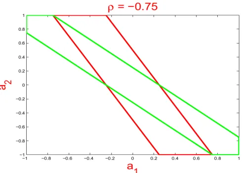
Figure 1: LetCSS and βS be as in Section 2.3 Example 2, whereρ=−0.75. For a row ofCNS, say,(a1,a2). The interior of the parallelogram and that of the hexagon are the regions of (a1,a2) satisfying the conditions of the lasso and marginal regression, respectively; see Example 1.

for which the respective conditions are satisfied. The two regions show significant overlap, and to a large extent, the conditions continue to overlap asρandβS vary. Examples for larger s can be constructed by lettingCSSbe a block diagonal matrix, where the size of each main diagonal block is small. For each row ofCNS, the conditions for the lasso and marginal regression are similar to those above, though more complicated.

Example 2. In the special case whereβS∝1S, Condition I for the lasso becomes|CNSCSS−11N| ≤ 1N, where the inequality should be interpreted as holding component-wise, and the condition for marginal regression (Condition F) is max_{|CNS1S|} ≤ min{|CSS1S|}. Note that if in addition 1Sis an eigen-vector ofCSS, then the two conditions are equivalent to each other. This includes but is not limited to the case ofs=2.

Example 3. Fixnand consider the special case in whichCSS=I. For the lasso, Condition E’ (and thus E) is satisfied, Condition J’ reduces toλ<ρ, and Condition I becomes_kCNSk ≤1. Under these conditions, the lasso gives exact reconstruction, but Condition F can fail. To see how, let

e

β_{∈ {−}1,1_}s_{be the vector such that max|C}

NSeβ|=kCNSk∞and letℓbe the index of the row at which

the maximum is attained, choosing the row with the biggest absolute element if the maximum is not unique. Letube the maximum absolute element of rowℓofCNSwith index j. Define a vectorδto be zero except in component j, which has the valueρeβj/(ukCNSk∞). Letβ=ρeβ+ρδ. Then,

|(CNSβ)ℓ|=ρ

kCNSk∞+

1

kCNSk∞

>ρ=min_|βS|,

so Condition F fails.

On the other hand, suppose Condition F holds for all βS∈ {−1,1}s. (It cannot hold for all

M

Choosingλ<ρ, we have Conditions E’, I, and J’ satisfied, showing by Theorem 1 that the lasso gives exact reconstruction. It follows that the conditions for the lasso are weaker in this case.

Example 4. For simplicity, assume thatβS∝1S, although the phenomenon to be described below is not limited to this case. For 1_≤i≤s, letλiandξi be thei-th eigenvalue and eigenvector ofCSS. Without loss of generality, we can takeξi to have unitℓ2norm. By elementary algebra, there are constantsc1, . . . ,cssuch that 1S=c1ξ1+c2ξ2+. . .+csξs. It follows that

C_SS−1_·1S= s

∑

i=1 ci

λi

ξi and CSS·1S= s

∑

i=1

(ciλi)ξi.

Fix a row ofCNS, say, a= (a1, . . . ,as). Respectively, the conditions for the lasso and marginal regression require

|(a, s

∑

i=1 ci

λi

ξi)| ≤1 and |(a,1S)| ≤ | s

∑

i=1

ciλiξi|. (6)

Without loss of generality, we assume thatλ1 is the smallest eigenvalue ofCSS. Consider the case whereλ1is small, while all other eigenvalues have a magnitude comparable to 1. In this case, the smallness ofλ1 has a negligible effect on ∑si=1(ciλi)ξi, and so has a negligible effect on the condition for marginal regression. However, the smallness ofλ1may have an adverse effect on the performance of the lasso. To see the point, we note that∑s_i=1ci

λiξi≈

c1

λ1ξ1. Compare this with the first term in (6). The condition for the lasso is roughly_|(a,ξ1)_{| ≤}c1λ1, which is rather restrictive sinceλ1is small.

Figure 2 shows the regions ina= (a1,a2,a3), a row ofCNS, where the respective exact recover sequences hold for

CSS=

 

1 ₋1/2 c

−1/2 1 0

c 0 1

 .

To better visualize these regions, we display their 2-D section (i.e., setting the first coordinate of ato 0). The Figures suggest that asλ1 gets smaller, the region corresponding to the lasso shrinks substantially, while that corresponding to marginal regression remains the same.

While the examples in this subsection are low dimensional, they shed light on the high di-mensional setting as well. For instance, the approach here can be extended to the following high-dimensional model: (a)_|sgn(βj)|iid∼Bernoulli(ε), (b) each row of the design matrixX are iid sam-ples fromN(0,Ω/n), whereΩis a p_×pcorrelation matrix that is sparse in the sense that each row ofΩhas relatively few coordinates, and (c) 1_≪pε_≪n_≪ p(note thatpεis the expected number of signals). Under this model, it can be shown that (1)CSSis approximately a block-wise diagonal matrix where each block has a relatively small size, and outside these blocks, all coordinates ofCSS are uniformly small and have a negligible effect, and (2) each row ofCNS has relatively few large coordinates. As a result, the study on the exact reconstruction conditions for the lasso and marginal regression in this more complicated model can be reduced to a low dimensional setting, like those discussed here. And the point that there is no clear winner between the to procedures continues to hold in greater generality.

2.4 Exact Reconstruction Conditions for Marginal Regression in the Noisy Case

We now turn to the noisy case of model (1), takingzto beN(0,σ2

n·In), where we assume that the parameterσ2

Figure 2: The regions sandwiched by two hyper-planes are the regions ofa= (a1,a2,a3)satisfying the respective exact-recovery conditions for marginal regression (MR, panel 1) and for the lasso (panels 2–4). See Section 2.3 Example 4. Here,c=0.5,0.7,0.85 and the smallest eigenvalues ofCSS areλ1(c) =0.29,0.14,0.014. As c varies, the regions for marginal regression remain the same, while the regions for the lasso get substantially smaller.

studied extensively in the literature (see for example Tibshirani, 1996). So in this section, we focus on marginal regression. First, we consider a natural extension of Condition F to the noisy case:

Condition F′. max_|CNSβS|+2σn

p

2 logp<min_|CSSβS|. (7)

Second, when Condition F’ holds, we show that with an appropriately chosen thresholdt(see (3)), marginal regression fully recovers the support with high probability. Finally, we discuss how to determine the thresholdtempirically.

Condition F’ implies that it is possible to separate relevant variables from irrelevant variables with high probability. To see this, letX = [x1,x2, . . . ,xp], wherexi denotes the i-th column ofX. Sort_|(Y,xi)|in the descending order, and letri=ri(Y,X)be the ranks of|(Y,xi)|(assume no ties for simplicity). Introduce

b

Sn(k) =Sbn(k;X,Y,p) ={i: ri(X,Y)≤k}, k=1,2, . . . ,p.

Recall thatS(β)denotes the support ofβands=_|S_|. The following lemma says that, ifsis known and Condition F’ holds, then marginal regression is able to fully recover the support Swith high probability.

Lemma 4 Consider a sequence of regression models as in (4). If for sufficiently large n, Condition F’ holds and p(n)_≥n, then

lim n_→∞P

b

Sn(s(n);X(n),Y(n),p(n))6=S(β(n))

Figure 3: Displayed are the 2-D sections of the regions in Figure 2, where we set the first coordinate ofato 0. Ascvaries, the regions for marginal regression remain the same, but those for the lasso get substantially smaller asλ1(c)decrease. x-axis: a2. y-axis:a3.

Lemma 4 is proved in Section 6. We remark that if bothsand(p₋s)tend to∞asntends to∞, then Lemma 4 continues to hold if we replace 2σn√2 logpin (7) byσn(

p

log(p₋s) +√logs). See the proof of the lemma for details.

The key assumption of Lemma 4 is that sis known so that we know how to set the threshold t. Unfortunately,s is generally unknown. We propose the following procedure to estimates. Fix 1_≤k_≤p, letikbe the unique index satisfyingrik(X,Y) =k. LetVbn(k) =Vbn(k;X,Y,p)be the linear

space spanned byxi1,xi2, . . . ,xik, and letHbn(k) =Hbn(k;X,Y,p)be the projection matrix fromR

n_to

b

Vn(k)(here and below, thebsign emphasizes the dependence of indicesik on the data). Define

b

δn(k) =bδn(k;X,Y,p) =k(Hbn(k+1)−Hbn(k))Yk, 1≤k≤p−1.

The termbδ2

n(k)is closely related to the F-test for testing whetherβik+1 6=0. We estimatesby

b

sn=bsn(X,Y,p) =max

1_≤k_≤p: bδn(k)≥σn

p

2 logn

+1

(in the case whereδbn(k)<σn√2 lognfor allk, we definebsn=1). Once_bsnis determined, we estimate the supportSby

b

S(_bsn,X,Y,p) ={ik:k=1,2, . . . ,bsn}.

It turns out that under mild conditions, _bsn=s with high probability. In detail, suppose that the supportS(β)consists of indices j1,j2, . . . ,js. Fix 1≤k≤s. LetVeS be the linear space spanned by xj1, . . . ,xjs, and letVeS,(−k)be the linear space spanned byxj1, . . . ,xjk−1,xjk+1, . . . ,xjs. Projectβjkxjk

other predictors removed), and let

∆∗_n(β,X,p) = min

1≤k≤s∆n(k,β,X,p).

The following theorem says that if ∆∗_n(β,X,p)is slightly larger than σn√2 logn, then bsn=sand

b

Sn=S with high probability. In other words, marginal regression fully recovers the support with high probability. Theorem 5 is proved in Section 6.

Theorem 5 Consider a sequence of regression models as in (4). Suppose that for sufficiently large n, Condition F’ holds, p(n)_≥n, and

lim n→∞

∆∗_n(β(n)_,X(n)_,p(n)₎

σn −

p

2 logn

=∞.

Then

lim n→∞P

b

sn(X(n),Y(n),p(n))6=s(n)

→0,

and

lim n→∞

b

Sn(bsn(X(n),Y(n),p(n));X(n),Y(n),n,p(n))6=S(β(n))

→0.

Theorem 5 says that the tuning parameter for marginal regression (i.e., the thresholdt) can be set successfully in a data driven fashion. In comparison, how to set the tuning parameterλfor the lasso has been a longstanding open problem in the literature.

We briefly discuss the case where the noise variance σ2

n is unknown. The topic is addressed in some of recent literature (e.g., Cand´es and Tao, 2007; Sun and Zhang, 2011). It is noteworthy that in some applications,σ2

ncan be calibrated during data collection and so it can be assumed as known (Cand´es and Tao, 2007, Rejoinder). It is also noteworthy that in Sun and Zhang (2011), they proposed a procedure to jointly estimateβandσ2

nusing scaled lasso. The estimator was show to be consistent withσ2

n in rather general situations, but unfortunately it is computationally more expensive than either the lasso or marginal regression. How to find an estimator that is consistent withσ2

nin general situations and has low computational cost remains an open problem, and we leave the study to the future.

With that being said, we conclude this section by mentioning that both the lasso and marginal regression have their strengths and weakness, and there is no clear winner between these two in general settings. For a given data set, whether to use one or the other is a case by case decision, where a close investigation of(X,β)is usually necessary.

3. The Deterministic Design, Random Coefficient Regime

is that it aims to control the worst case so it is conservative. In this section, we derive a condition— Condition F”—which can be viewed as a middle ground between the Faithfulness Condition and the Incoherence Condition: it is not tied to the unknown support so it is more tractable than the Faithfulness Condition, and it is also much less stringent than the Incoherence Condition.

In detail, we modelβas follows. Fixε_∈(0,1),a>0, and a distributionπ, where

the support ofπ _⊂(₋∞,₋a]_∪[a,∞). (8)

For each 1_≤i_≤p, we draw a sampleBi from Bernoulli(ε). WhenBi=0, we setβi=0. When Bi=1, we drawβi∼π. Marginally,

βi iid

∼(1₋ε)ν0+επ, (9)

whereν0 denotes the point mass at 0. This models the case where we have no information on the signals, so they appear at locations generated randomly. In the literature, it is known that the least favorable distribution for variable selection has the form as in (9), whereπis in fact degenerate. See Cand`es and Plan (2009) for example.

We study for which quadruples(X,ε,π,a)the Faithfulness Condition holds with high probabil-ity. Recall that the design matrixX= [x1, . . . ,xp], wherexi denotes thei-th column. Fixt≥0 and

δ>0. Introduce

gi j(t) =Eπ[etu·(xi,xj)]−1, g¯i(t) =

∑

gi j(t),

where the random variableu_∼πand(xi,xj)denotes the inner product ofxi andxj. As before, we have suppressed the superscript (n)forgi j(t)and ¯gi(t). Define

An(δ,ε,g) =¯ An(δ,ε,g;¯ X,π) =min t>0

e−δt p

∑

i=1

[eεg¯i(t)_+eεg¯i(−t)_]

,

where ¯gdenotes the vector(g¯1, . . . ,g¯p)T. Note that 1+gi j(t)is the moment generating function ofπ evaluated at the point(xi,xj)t. In the literature, it is conventional to use moment generating function to derive sharp inequalities on the tail probability of sums of independent random variables. The following lemma is proved in Section 6.

Lemma 6 Fix n, X ,δ>0,ε_∈(0,1), and distributionπ. Then

P(max_|CNSβS| ≥δ)≤(1−ε)An(δ,ε,g;X¯ ,π), (10)

and

P(max_|(CSS−IS)βS| ≥δ)≤εAn(δ,ε,g;X,¯ π). (11) Now, suppose the distribution πsatisfies (8) for somea>0. Takeδ=a/2 on the right hand side of (10)-(11). Except for a probability ofAn(a/2,ε,g),¯

max_|CNSβS| ≤a/2, min|CSSβS| ≥min|βS| −max|(CSS−I)βS| ≥a/2,

so max_|CNSβS| ≤min|CSSβS|and the Faithfulness Condition holds. This motivates the following condition, where(a,ε,π)may depend onn.

Condition F′′. lim

n→∞An(an/2,εn,g¯

(n)_;X(n)_,π

n) =0.

Theorem 7 Consider a sequence of noise-free regression models as in (4), where the noise compo-nent z(n)=0andβ(n)_{is generated as in (9). Suppose Condition F” holds. Then as n tends to∞,}

except for a probability that tends to0,

max_|CNSβS| ≤min|CSSβS|.

Theorem 7 is the direct result of Lemma 6 so we omit the proof.

3.1 Comparison of Condition F” with the Incoherence Condition

Introduced in Donoho and Elad (2003) (see also Donoho and Huo, 2001), the Incoherence of a matrixXis defined as

max i₆=j |Ci j|,

whereC=XTX is the Gram matrix as before. The notion is motivated by the study in recovering a sparse signal from an over-complete dictionary. In the special case whereX is the concatenation of two orthonormal bases (e.g., a Fourier basis and a wavelet basis), maxi6=j|Ci j|measures how coherent two bases are and so the term of incoherence; see Donoho and Elad (2003) and Donoho and Huo (2001) for details. Consider Model (1) in the case where bothX andβare deterministic, and the noise componentz=0. The following results are proved in Chen et al. (1998), Donoho and Elad (2003) and Donoho and Huo (2001).

• The lasso yields exact variable selection ifs<1+maxi6=j|Ci j|

2 maxi6=j|Ci j| . • Marginal regression yields exact variable selection if s< _{2 max}c

i6=j|Ci j| for some constantc∈

(0,1), and that the nonzero coordinates ofβhave comparable magnitudes (i.e., the ratio be-tween the largest and the smallest nonzero coordinate ofβis bounded away from∞).

In comparison, the Incoherence Condition only depends on X so it is checkable. Condition F depends on the unknown support ofβ. Checking such a condition is almost as hard as estimating the supportS. Condition F” provides a middle ground. It depends onβ only through(ε,π). In cases where we either have a good knowledge of(ε,π)or we can estimate them, Condition F” is checkable (for literature on estimating(ε,π), see Jin, 2007 and Wasserman, 2006 for the case where we have an orthogonal design, and Ji and Jin, 2012, Section 2.6 for the case whereXTX is sparse in the sense that each row ofXTX has relatively few large coordinates. We note that even when successful variable selection is impossible, it may be still possible to estimate(ε,π)well).

At the same time, the Incoherence Condition is conservative, especially whensis large. In fact, in order for either the lasso or marginal regression to have an exact variable selection, it is required that

max

i₆=j |Ci j| ≤O

1 s

,

In other words, all coordinates of the Gram matrixC need to be no greater thanO(1/s). This is much more conservative than Condition F.

Incoherence Condition, applying more broadly than the former, while being less conservative than the later.

Below, we use two examples to illustrate that Condition F” is much less conservative than the Incoherence Condition. In the first example, we consider a weakly dependent case where maxi6=j|Ci j| ≤O(1/log(p)). In the second example, we suppose the matrixC is sparse, but the nonzero coordinates ofCmay be large.

3.1.1 THEWEAKLYDEPENDENT CASE

Suppose that for sufficiently largen, there are two sequence of positive numbersan≤bnsuch that the support ofπnis contained in[−bn,−an]∪[an,bn], and that

bn an·

max

i6=j |Ci j| ≤c1/log(p), c1>0 is a constant. Fork_≥1, denote thek-th moment ofπnby

µ(nk)=µ(nk)(πn).

Introducemn=mn(X)andv2n=v2n(X)by mn(X) =pεn·max

1≤i≤p

1 p

∑

, v2_n(X) =pεn·max 1≤i≤p

1 p

∑

2 i j

.

Corollary 3.1 Consider a sequence of regression models as in (4), where the noise component z(n)=0andβ(n)_{is generated as in (9). If there are constants c1>0and c2∈(0,1/2)such that}

bn an·

max

i₆=j {|Ci j|} ≤c1/log(p

(n)_),

and

lim n→∞

µ(n1)(πn) an

mn(X(n))

≤c2, lim n→∞

µ(n2)(πn) a2

n

v2_n(X(n))log(p(n))

=0, (12)

then

lim

n→∞An(an/2,εn,g¯

(n)_;X(n)_,π

n) =0,

and Condition F” holds.

Corollary 3.1 is proved in Section 6. For interpretation, we consider the special case where there is a generic constantc>0 such thatbn≤can. As a result,µ(n1)/an≤c,µ(n2)/a2n≤c2. The conditions reduce to that, for sufficiently largenand all 1_≤i_≤p,

|1_p

p

∑

j6=i

Ci j| ≤O( 1 pεn

), 1 p

p

∑

j6=i

C2_{i j}=o(1/pεn).

Note that by (9),s=s(n)_∼Binomial(p,εn), sos≈pεn. Recall that the Incoherence Condition is

max

i6=j |Ci j| ≤O(1/s).

3.1.2 THESPARSECASE

LetN_n∗(C)be the maximum number of nonzero off-diagonal coordinates ofC:

N_n∗(C) = max

1≤i≤p{Nn(i)}, Nn(i) =Nn(i;C) =#{j: j6=i,Ci j6=0}. Suppose there is a constantc3>0 such that

lim n→∞

−log(εnNn∗(C)) log(p(n)₎

≥c3. (13)

Also, suppose there is a constantc4>1 such that for sufficiently largen,

the support ofπnis contained in[−c4an,an]∪[an,c4an]. (14)

The following corollary is proved in Section 6.

Corollary 3.2 Consider a sequence of noise-free regression models as in (4), where the noise com-ponent z(n)=0 andβ(n) _{is randomly generated as in (9). Suppose (13)-(14) hold. If there is a}

constantδ>0such that

max

i6=j |Ci j| ≤δ, and δ< c3 2c4, then

lim

n→∞An(an/2,εn,g¯

(n)_;X(n)_,π

n) =0,

and Condition F” holds.

For interpretation, consider a special case whereεn=p−ϑ. In this case, the condition reduces toN_n∗(C)_≪pϑ−2c4δ_{. As a result, Condition F” is satisfied if each row of(C−I)contains no more} than pϑ−2c4δ _{nonzero coordinates each of which ≤δ. Compared to the Incoherence Condition} maxi6=j|Ci j| ≤O(1/s) =O(p−ϑ), our condition is much weaker.

In conclusion, if we alter our attention from the worst-case scenario to the average scenario, and alter our aim from exact variable selection to exact variable selection with probability _≈1, then the condition required for success—Condition F”—is much more relaxed than the Incoherence Condition.

4. Hamming Distance for the Gaussian Design and the Phase Diagram

So far, we have focused on exact variable selection. In many applications, exact variable selection is not possible. Therefore, it is of interest to study the Type I and Type II errors of variable selection (a Type I error is a misclassified 0 coordinate ofβ, and a Type II error is a misclassified nonzero coordinate).

In this section, we use the Hamming distance to measure the variable selection errors. Back to Model (1),

Y=Xβ+z, z∼N(0,In), (15)

where without loss of generality, we assume σn=1. As in the preceding section (i.e., (9)), we suppose

βi iid

For any variable selection procedurebβ=bβ(Y;X), the Hamming distance betweenbβand the trueβ

is

d(bβ_|X) =d(bβ;ε,π_|X) = p

∑

j=1

Eε,π(Ez[1(sgn(bβj)6=sgn(βj))|X]).

Note that by Chebyshev’s inequality,

P(non-exact variable selection bybβ(Y;X))_≤d(bβ_|X).

So a small Hamming distance guarantees exact variable selection with high probability.

How to characterize precisely the Hamming distance is a challenging problem. We approach this by modelingX as random. Assume that the coordinates ofX are iid samples fromN(0,1/n):

Xi j iid

∼N(0,1/n). (16)

The choice of the variance ensures that most diagonal coordinates of the Gram matrixC=XTXare approximately 1. LetPX(x)denote the joint density of the coordinates ofX. The expected Hamming distance is then

d∗(bβ) =d∗(bβ;ε,π) = Z

d(bβ;ε,π_|X =x)PX(x)dx.

We adopt an asymptotic framework where we calibrate pandεwith

p=n1/θ, pεn=n(1−ϑ)/θ≡p1−ϑ, 0<θ,ϑ<1. (17) This models a situation wherep_≫nand the vectorβgets increasingly sparse asngrows. Note that the parameterϑcalibrates the sparsity level of the signals. We assumeπnin (9) is a point mass

πn=ντn. (18)

In the literature (e.g., Donoho and Jin, 2004; Meinshausen and Rice, 2006), this model was found to be subtle and rich in theory. In addition, compare two experiments, in one of themπn=ντn, and

in the other the support ofπnis contained in[τn,∞). Since the second model is easier for inference than the first one, the optimal Hamming distance for the first one gives an upper bound for that for the second one.

With εn calibrated as above, the most interesting range for τn is O(√2 logp): when τn ≫

√

2 logp, exact variable selection can be easily achieved by either the lasso or marginal regres-sion. Whenτn≪√2 logp, no variable selection procedure can achieve exact variable selection. See, for example, Donoho and Jin (2004). In light of this, we calibrate

τn=

p

2(r/θ)logn_≡p2rlogp, r>0. (19)

Note that the parameterrcalibrates the signal strength. With these calibrations, we can rewrite

d_n∗(bβ;ε,π) =d_n∗(bβ;εn,τn).

Definition 8 Denote L(n)by a multi-log term which satisfies that limn→∞(L(n)·nδ) =∞and that

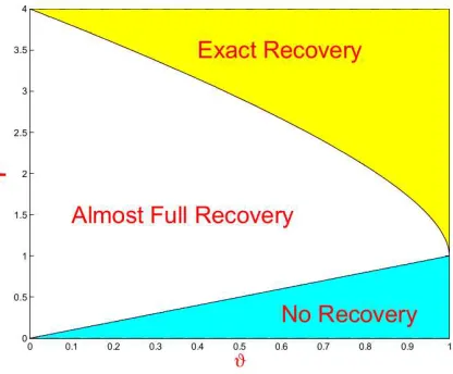
Figure 4: The regions as described in Section 4. In the region of Exact Recovery, both the lasso and marginal regression yield exact recovery with high probability. In the region of Almost Full Recovery, it is impossible to have large probability for exact variable selection, but the Hamming distance of both the lasso and marginal regression_≪ pεn. In the region of No Recovery, optimal Hamming distance_∼pεnand all variable selection procedures fail completely. Displayed is the part of the plane corresponding to 0<r<4 only.

We are now ready to spell out the main results. Define

ρ(ϑ) = (1+√1₋ϑ)2, 0<ϑ<1.

The following theorem is proved in Section 6, which gives the lower bound for the Hamming dis-tance.

Theorem 9 Fix ϑ _∈(0,1), θ>0, and r >0 such that θ>2(1₋ϑ). Consider a sequence of regression models as in (15)-(19). As n_→∞, for any variable selection procedurebβ(n)_,

d∗_n(bβ(n);εn,τn)≥

(

L(n)p1₋(ϑ+_4rr)2_{, r≥ϑ,} (1+o(1))_·p1−ϑ, 0<r<ϑ. Letbβmr be the estimate of using marginal regression with threshold

tn=

( _ϑ+r

2√r

√

2 logp, ifr>ϑ, tn=

p

2_erlogp, ifr<ϑ, (20)

where_eris some constant_∈(ϑ,1)(note that in the case ofr<ϑ, the choice oftnis not necessarily unique). We have the following theorem.

(20) satisfies

d∗_n(bβmr(n);εn,τn)≤

(

L(n)p1₋(ϑ+_4rr)2_{, r≥ϑ,} (1+o(1))_·p1−ϑ, 0<r<ϑ.

In practice, the parameters(ϑ,r)are usually unknown, and it is desirable to settn in a data-driven fashion. Towards this end, we note that our primary interest is in the case ofr>ϑ(as whenr<ϑ, successful variable selection is impossible). In this case, the optimal choice oftnis(ϑ+r)/(2r)τp, which is the Bayes threshold in the literature. The Bayes threshold can be set by the approach of controlling the local False Discovery Rate (Lfdr), where we set the FDR-control parameter as 1/2; see Efron et al. (2001) for details.

Similarly, choosing the tuning parameter λn=2(ϑ₂√+r_r∧√r)√2 logp in the lasso, we have the following theorem.

Theorem 11 Fixϑ_∈(0,1), r>0, andθ>(1₋ϑ). Consider a sequence of regression models as in (15)-(19). As p_→∞, the Hamming distance of the lasso with the tuning parameterλn=2tnwhere tnis given in (20), satisfies

d_n∗(bβ_lasso(n) ;εn,τn)≤

(

L(n)p1−(ϑ+4rr)2, r≥ϑ,

(1+o(1))_·p1−ϑ, 0<r<ϑ. The proofs of Theorems 10-11 are routine and we omit them.

Theorems 9-11 say that in theϑ-rplane, we have three different regions, as displayed in Figure 4.

• Region I (Exact Recovery): 0<ϑ<1 andr>ρ(ϑ).

• Region II (Almost Full Recovery): 0<ϑ<1 andϑ<r<ρ(ϑ).

• Region III (No Recovery): 0<ϑ<1 and 0<r<ϑ.

In the Region of Exact Recovery, the Hamming distance for both marginal regression and the lasso are algebraically small. Therefore, except for a probability that is algebraically small, both marginal regression and the lasso give exact recovery.

In the Region of Almost Full Recovery, both the Hamming distance of marginal regression and the lasso are much smaller than the number of relevant variables (which_≈pεn). Therefore, almost all relevant variables have been recovered. Note also that the number of misclassified irrelevant variables is comparably much smaller than pεn. In this region, the optimal Hamming distance is algebraically large, so for any variable selection procedure, the probability of exact recovery is algebraically small.

In the Region of No Recovery, the Hamming distance_∼pεn. In this region, asymptotically, it is impossible to distinguish relevant variables from irrelevant variables, and any variable selection procedure fails completely.

In practice, given a data set, one wishes to know that which of these three regions the true parameters belong to. Towards this end, we note that in the current model, the coordinates ofXTY are approximately iid samples from the following two-component Gaussian mixture

where φ(x) denotes the density of N(0,1). In principle, the parameters (εn,τn) can be estimated (see the comments we made in Section 3.1 on estimating(ε,π)). The estimation can then be used to determine which regions the true parameters belong to.

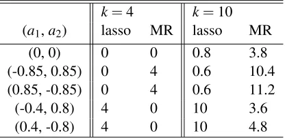
k=4 k=10

(a1,a2) lasso MR lasso MR

(0, 0) 0 0 0.8 3.8

(-0.85, 0.85) 0 4 0.6 10.4 (0.85, -0.85) 0 4 0.6 11.2 (-0.4, 0.8) 4 0 10 3.6 (0.4, -0.8) 4 0 10 4.8

Table 1: Comparison of the lasso and marginal regression for different choices of(a1,a2)andk. The setting is described in Experiment 1a. Each cell displays the corresponding Hamming error.

The results improve on those by Wainwright (2006). It was shown in Wainwright (2006) that there are constantsc2>c1>0 such that in the region of_{0<ϑ<1,r>c2_}, the lasso yields exact variable selection with overwhelming probability, and that in the region of_{0<ϑ<1,r<c2_}, no procedure could yield exact variable selection. Our results not only provide the exact rate of the Hamming distance, but also tighten the constantsc1 andc2so thatc1=c2= (1+√1−ϑ)2_{. The} lower bound argument in Theorem 9 is based on computing theL1-distance. This gives better results than in Wainwright (2006) which uses Fano’s inequality in deriving the lower bounds.

To conclude this section, we briefly comment on the phase diagram in two closely related set-tings. In the first setting, we replace the identity matrixIpin (16) by some general correlation matrix

Ω, but keep all other assumptions unchanged. In the second setting, we assume that asn_→∞, both ratios pεp/nandn/ptend to a constant in(0,1), while all other assumptions remain the same. For the first setting, it was shown in Ji and Jin (2012) that the phase diagram remains the same as in the case ofΩ=Ip, provided thatΩis sparse; see Ji and Jin (2012) for details. For the second setting, the study is more more delicate, so we leave it to the future work.

5. Simulations and Examples

We conducted a small-scale simulation study to compare the performance of the lasso and marginal regression. The study includes three different experiments (some have more than one sub-experiments). In the first experiment, the rows of X are generated from N(0,1

nC) where C is a diagonal block-wise matrix. In the second one, we take the Gram matrixC=X′X to be a tridiagonal matrix. In the third one, the Gram matrix has the form ofC=Λ+aξξ′ whereΛ is a diagonal matrix,a>0, andξis a p_×1 unit-norm vector. Intrinsically, the first two are covered in the theoretic discussion in Section 2.3, but the last one goes beyond that. Below, we describe each of these experiments in detail.

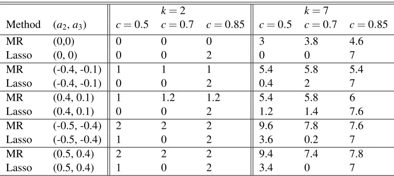
k=2 k=7

Method (a2,a3) c=0.5 c=0.7 c=0.85 c=0.5 c=0.7 c=0.85

MR (0,0) 0 0 0 3 3.8 4.6

Lasso (0, 0) 0 0 2 0 0 7

MR (-0.4, -0.1) 1 1 1 5.4 5.8 5.4

Lasso (-0.4, -0.1) 0 0 2 0.4 2 7

MR (0.4, 0.1) 1 1.2 1.2 5.4 5.8 6

Lasso (0.4, 0.1) 0 0 2 1.2 1.4 7.6

MR (-0.5, -0.4) 2 2 2 9.6 7.8 7.6

Lasso (-0.5, -0.4) 1 0 2 3.6 0.2 7

MR (0.5, 0.4) 2 2 2 9.4 7.4 7.8

Lasso (0.5, 0.4) 1 0 2 3.4 0 7

Table 2: Comparison of the lasso and marginal regression for different choices of(c,a2,a3). The setting is described in Experiment 1b. Each cell displays the corresponding Hamming error.

N(0,(1/n)C), whereCis a diagonal block-wise correlation matrix having the form

C=

   

C_sub 0 0 . . .0 0 C_sub 0 . . .0

. . . .

0 0 0 . . .C_sub

   .

Fixing a small integerm, we takeC_{sub to be the}m_×mmatrix as follows:

C_sub=

D aT a 1

,

where a is an (m₋1)_×1 vector and D is an (m₋1)_×(m₋1) matrix to be introduced below. Also, fixing another integerk_≥1, according to the block-wise structure ofC, we letβbe the vector (without loss of generality, we assumepis divisible bym)

β= (δ1uT,δ2uT, . . . ,δ_p/muT)T, whereu= (vT_{,0)for some(m−1)×1 vectorvandδ}

i=0 for all butkdifferenti, whereδi=1. The goal of this experiment is to investigate how the theoretic results in Section 2.3 shed light on models with more practical interests. To see the point, note that whenk_≪n, the signal vectorβ

is sparse, and we expect to see that

X′Xβ_≈Cβ, (21)

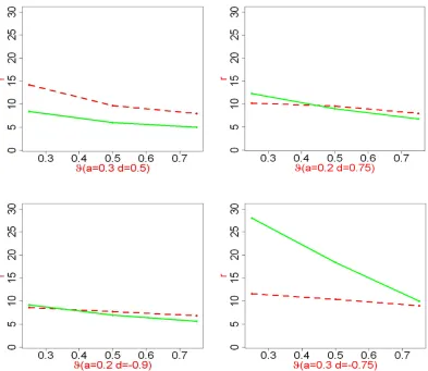
Figure 5: Critical values of exact recovery for the lasso (dashed) and marginal regression (solid). See Experiment 2 for the setting and the definition of critical value. For any given set of parameters(ϑ,a,d), the method with a smaller critical value has the better performance in terms of Hamming errors.

In Experiment 1a, we take(p,n,m) = (999,900,3). At the same time, for some numbersa1and a2, we seta,v, andDby

a= (a1,a2)T, v= (2,1)T, D=

1 ₋.75

−.75 1

.

Consider for a second the idealized case whereX′X=C(i.e.,nis very large). If we restrict our attention to any block ofβwhere the correspondingδi is 1, the setting reduces to that of Example 1 of Section 2.3. In fact, in Figure 1, our first choice of(a1,a2)falls inside both the parallelogram and hexagon, our next two choices fall inside the hexagon but outside the parallelogram, and our last two choices fall outside the hexagon but inside the parallelogram. Therefore, at least whenk is sufficiently small (so that the setting can be well-approximated by that in the idealized case), we expect to see that the lasso outperforms marginal regression with the second and the third choices, and expect to see the other way around with the last two choices of(a1,a2). In the first choice, both methods are expected to perform well.

We now investigate how well these expectations are met. For each combination of these parame-ters, we generate data and compare the Hamming errors of the lasso and marginal regression, where for each method, the tuning parameters are set ideally. The ‘ideal’ tuning parameter is obtained through rigorous search from a range. The error rates over 10 repetitions are tabulated in Table 1. More repetitions is unnecessary, partially because the standard deviations of the simulation results are small, and partially because the program is slow (for that we need to choose the ‘ideal’ tuning parameter through rigorous search. Take the lasso for example. For rigorous search of the ‘ideal’ tuning parameter, we need to run the glmnet R package many times).

The results suggest that the performances of each method are reasonably close to what are ex-pected for the idealized model, especially in the case of k = 4. Take the cases (a1,a2) =

±(0.85,₋0.85)for example. The lasso yields exact recovery, while marginal regression, in each of the four blocks where the correspondingδi is 1, recovers correctly the stronger signal and mistak-enly kills the weaker one. The situation is reversed in the cases where(a1,a2) =±(0.4,−0.8). The discussion for the case ofk=10 is similar, but the approximation error in Equation (21) starts to kick in.

In Experiment 1b, we take(p,n,m) = (900,1000,4). Also, for some numbersc,a2, anda3, we seta,v, andDas

aT = (0,a2,a3)T, v= (1,1,1)T, D=

 

1 ₋1/2 c

−1/2 1 0

c 0 1

 .

The primary goal of this experiment is to investigate how different choices ofc affect the perfor-mance of the lasso and marginal regression. To see the point, note that in the idealized situation where X′X =C, the model reduces to the one discussed in Figure 3, if we restrict our attention to any block of β whereδi=1. The theoretic results in Example 4 of Section 2.3 predict that, the performance of the lasso gets increasingly unsatisfactory ascincreases, while that of marginal regression stay more or less the same. At the same time, which of this method performs better depends on(a2,a3,c), see Figure 3 for details.

not have a big influence over marginal regression. The results fit well with the theory illustrated in Section 2.3; see Figure 3 for comparisons.

Experiment 2. In this experiment, we use the linear regression modelY =Xβ+z where z_∼ N(0,In). We use a different criterion rather than the Hamming errors to compare two methods: with the same parameter settings, the method that yields exact recovery in a larger range of parameters is better. Towards this end, we take p=n=500, andX=Ω1/2_{, whereΩis the p×ptridiagonal} matrix satisfying

Ω(i,j) =1_{i= j_}+a_·1_{|i₋j_|=1_},

and the parametera_∈(₋1/2,1/2)so the matrix is positive definite. At the same time, we generate

β as follows. Letϑ range between 0.25 and 0.75 with an increment of 0.25. For each ϑ, let s be the smallest even number _≥ p1−ϑ. We then randomly pick s/2 indices i1 <i2 < . . . <is/2. For parameters r>0 and d _∈(₋1,1) to be determined, we let τ=√2rlogp and let βj =τ if

j_{∈ {}i1,i2, . . . ,is/2},βj=dτif j−1∈ {i1,i2, . . . ,is/2}, andβj=0 otherwise.

To gain insight on how two procedures perform in this setting, we consider the noiseless counter-part for just a second. Without loss of generality, we assume that the minimum inter-distance of in-dicei1,i2, . . . ,ik≥4. LetYe=X′Y. For anyik, 1≤k≤s/2, if we restrictYeto{ik−1,ik,ik+1,ik+2} and call the resulting vectory, then

y=Aα,

whereAis the 4 matrix satisfyingA(i,j) =1{i= j}+a·1{|i−j|=1}, 1≤i,j≤4, andαis the 4_×1 vector such thatα1=α4=0,α2=τ, andα3=dτ. In this simple model, the performance of the lasso and marginal regression can be similarly analyzed as in Section 2.3.

Now, for each of the combination of(d,ϑ), we use the method of exhausting search to determine the smallestrsuch that the lasso or marginal regression yields exact recovery with 50 repetition of simulations, respectively (similarly, the tuning parameters of each method are set ideally). For each method, we call the resultant value ofrthecritical value for exact recovery. For eachϑand choices of(a,d), we find the critical values for both methods. The results are summarized in Figure 5. For a given triplet (ϑ,a,d), the method that gives a larger critical value is inferior to the one with a smaller critical value (as the region of parameters where it yields exact recovery is smaller). Figure 5 suggests that the parameters(a,d)play an important role in determining the performance of the lasso and marginal regression. For example, the performance of both procedures worsen when a get larger. This is because that asaincreases, the Gram matrix moves away from that the identity matrix, and the problem of variable selection becomes increasingly harder. Also, the sign ofa_·d plays an interesting role. For example, whena_·d <0, it is known that the marginal regression faces a so-called challenge of signal cancellation (see for example Wasserman and Roeder, 2009). It seems that the lasso handles signal cancellation better than does marginal regression. However, when(a,d)range, there is no clear winner between two methods.

Experiment 3. So far, we have focused on settings where the regression problem can be de-composed into many parallel small-size regression problems. While how to decompose remains unknown, such insight is valuable, as we can always compare the performance of two methods over each of these small-size regression problems using the theory developed in Section 2.3; the overall performance of each method is then the sum of that on these small-size problems.

z∼N(0,In). We takep=nandX =Ω1/2, whereΩis a correlation matrix having the form

Ω=Λ+aξξ′.

which is a rank one perturbation of the diagonal matrixΛ. Here, ξ is the p_×1 vector where its p/2 even coordinates are 1, and the remaining coordinates areb, wherea>0 andbare parameters calibrating the norm and direction of the rank one perturbation, respectively. Experiment 3 contains two sub-experiments, 3a and 3b.

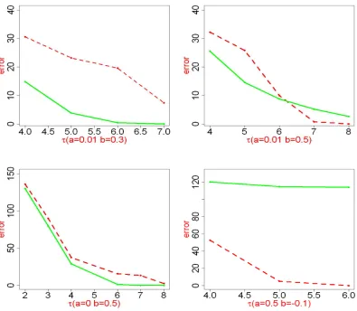
In Experiment 3a, we investigate how the choices of parameters (a,b)and the signal strength affect the performance of the lasso and marginal regression. Letp=n=3000, and letβi=τwhen i_{∈ {}k:k=8_×(ℓ₋1) +1,1_≤ℓ_≤150_}andβi=0 otherwise, whereτcalibrates the signal strength. For each of the four choices (a,b) = (0.01,0.3),(0.01,0.5),(0,0.5),(0.5,₋0.1), we compare the lasso and marginal regression forτ=2,3, . . . ,8. The Hamming errors are shown in Figure 6. The results suggest that the parameters(a,b) play a key role in the performance of both the lasso and marginal regression. For example, whenaincreases, the performance of both methods worsen, due to that the Gram matrix moves away from the identity matrix. Also, for relatively smalla, it seems that marginal regression outperforms the lasso (see Panel 1 and 2 of Figure 6).

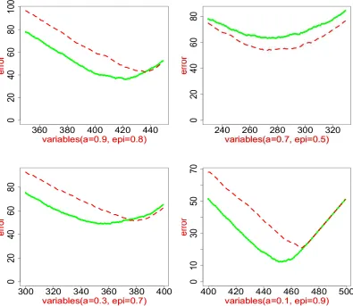
In Experiment 3b, we take a different angle and investigate how the levels of the signal sparsity affect the performance of the lasso and marginal regression. Consider a special case where where b=1. In this case, ξ reduces to the vector of ones, and the Gram matrix is an equi-correlation matrix. This setting can be found in many literature on variable selection. Taken=p=500. We generate the coordinates ofβfrom the mixing distribution of point mass at 0 and the point mass at

τ:

βi iid

∼(1₋ε)ν0+εντ,

whereεcalibrates the sparsity level andτcalibrates the signal strength (in this experiment, we take

τ=5). In Figure 7, we plot the Hamming errors of 10 repetition versus the number of variables retained (which can be thought of different choices of tuning parameters). Interestingly, it seems that the performance of two methods are strikingly similar, with relatively small differences (one way or the other) when the parameters(a,ε)are moderate (neither too close to 0 nor to 1). This is interesting as whenρis moderate, the design matrixXis significantly non-orthogonal. Additionally, the results suggest that the sparsity parameter ε has a major influence over the relative performance of two methods. Whenεget larger (so the signals get denser), marginal regression tends to outperform the lasso. The underlying reason is that when both the correlation and signals are positive, the strength of individual signals are amplified due to correlation, and so have a positive effect on marginal regression.

At the same time, it seems that the correlation parameter aalso have a major effect over the performance of two methods, and the error rate of both methods increase as a increases. How-ever, somewhat surprisingly, the parametera does not seem to have a major effect on the relative performance of two methods.

We conclude this section by mentioning that from time to time, one would like to know for the data at hand, which method is preferable. Generally, this is a hard problem, and generally, there is no clear winner between the lasso and marginal regression. However, there are something can be learned from these simulation examples.

Figure 6: Comparison of Hamming errors by the lasso (dashed) and marginal regression (solid). The setting is described in Experiment 3a.

Figure 7: Comparison of Hamming errors by the lasso (dashed) and marginal regression (solid). Thex-axis shows the number of retained variables. The setting is described in Experiment 3b.

6. Proofs

This section contains the technical proofs of all theorems and lemmas of the preceding sections.

6.1 Proof of Theorem 3

Defineβas follows:

βj=

    

ρDii

Di j if j6=iandDi j6=0 ρ if j₆=iandDi j=0

−kiρ if j=i..

Because_|Di j| ≤Dii, this satisfies|βj| ≥ρ, soβ∈

M

(Dβ)i=

∑

Di jβj=−kiDiiρ+

∑

j6=i Di j6=0

ρDii Di j

Di j=0.

This proves the theorem.

6.2 Proof of Lemma 4

By the definition ofSbn(s), it is sufficient to show that except for a probability that tends to 0,

max_|X_NTY_|<min_|X_STY_|.

Since Y =Xβ+z=XSβS+z, we have XNTY =XNT(XSβS+z) =CNSβS+XNTz. Note that xTi z∼ N(0,σ2

n). By Boolean algebra and elementary statistics,

P(max_|X_NTz_|>σn

p

2 logp)_≤

_∑

P(_|(xi,z)| ≥σn

p

2 logp)_≤√C

logp p₋s

p .

It follows that except for a probability ofo(1),

max_|X_NTY_{| ≤}max_|CNSβS|+max|XNTz| ≤max|CNSβS|+σn

p

2 logp.

Similarly, except for a probability ofo(1),

min_|X_STY_{| ≥}min_|CSSβS| −max|XSTz| ≥min|CSSβS| −σn

p

2 logp.

Combining these gives the claim.

6.3 Proof of Theorem 5

Once the first claim is proved, the second claim follows from Lemma 4. So we only show the first claim. Write for shortSbn(s) =Sbn(s(n);X(n),Y(n),p(n)), s=s(n), and S=S(β(n)). All we need to show is

lim

n→∞P(bsn6=s) =0.

Introduce the event

Dn={Sbn(s) =S}. It follows from Lemma 4 that

P(Dc_n)_→0.

Write

It is sufficient to show limn→∞P(bsn6=s|Dn) =0, or equivalently,

lim

n_→∞P(sbn>s|Dn) =0 and nlim_→∞P(bsn<s|Dn) =0. (22)

Consider the first claim of (22). Write for shorttn=σn√2 logn. Note that the event{bsn>s|Dn} is contained in the event of_∪kp₌−_s1_{bδn(k)≥tn|Dn}. RecallingP(Dcn) =o(1),

P(_bsn>s)≤ p−1

∑

k=s

(bδ(k)_≥tn|Dn). p−1

∑

k=s

P(bδn(k)≥tn), (23)

where we say two positive sequencesan.bnif limn→∞(an/bn)≤1.

Fixs_≤k_≤p₋1. By definitions,H(kb +1)₋H(k)b is the projection matrix fromRntoVbn(k+ 1)_∩Vbn(k)⊥. So conditional on the event {Vbn(k+1) =Vbn(k)}, δn(k) =0, and conditional on the event_{Vbn(k+1)(Vbn(k)},δ2n(k)∼σ2nχ2(1). Note thatP(χ2(1)≥ 2 logn) =o(1/n). It follows that

p₋1

∑

k=s

P(bδn(k)≥tn) = p₋1

∑

k=s

P(bδn(k)≥tn|Vbn(k)(Vbn(k+1))P(Vbn(k)(Vbn(k+1))

=o(1 n)

p₋1

∑

k=s

P(Vbn(k)(Vbn(k+1)). (24)

Moreover,

p−1

∑

k=s

P(Vbn(k)(Vbn(k+1)) = p−1

∑

k=s

E[1(dim(Vbn(k+1))>dim(Vbn(k)))]

=E[ p−1

∑

k=s

1(dim(Vbn(k+1))>dim(Vbn(k)))].

Note that for any realization of the sequencesVbn(1), . . . ,Vbn(p),∑_kp₌−_s11(dim(Vbn(k+1))>dim(Vbn(k)))

≤n. It follows that

p−1

∑

k=s

P(Vbn(k)(Vbn(k+1))≤n. (25)

Combining (23)-(25) gives the claim.

Consider the second claim of (22). By the definition ofsbn, the event{bsn<s|Dn)}is contained in the event_{bδn(s−1)<tn|Dn}. By definitions,bδn(s−1) =k(H(s)b −H(sb −1))Yk, wherek· k=k· k2 denotes theℓ2_{norm. So all we need to show is}

lim

n_→∞P(k(H(s)b −H(sb −1))Yk<tn|Dn) =0. (26)

Fix 1 _≤k _≤ p. Recall that ik denotes the index at which the rank of |(Y,xik)| among all |(Y,xj)|isk. DenoteXe(k) by the nby k matrix [xi1,xi2, . . . ,xik], and denoteeβ(k) by thek-vector

(βi1,βi2, . . . ,βik)

T_{. Conditional on the eventD}

n,Sbn(s) =S, andβi1,βi2, . . . ,βis are all the nonzero

coordinates ofβ. So according to our notations,

Now, first, note thatH(s)b Xe(s) =X(s)e andH(sb ₋1)Xe(s₋1) =Xe(s₋1). Combine this with (27). It follows from direct calculations that

(H(s)b ₋H(sb ₋1))Xβ= (I₋H(sb ₋1))xis. (28)

Second, sincexis∈Vbn(s),(I−H(s))xb is =0. So

(I₋Hbs−1)xis = (I−H(s))xb is+ (H(s)b −H(sb −1))xis= (Hbs−Hbs−1)xis. (29)

Last, splitxisinto two terms,xis=x (1)

is +x (2)

is such thatx (1)

is ∈Vbn(s−1)andx (2)

is ∈Vbn(s)∩(Vbn(s−1))

⊥_.

It follows that(H(s)b ₋H(sb ₋1))x(_i1)

s =0, and so

(H(s)b ₋H(sb ₋1))xis= (H(s)b −H(sb −1))x (2)

is . (30)

Combining (28)-(30) gives

(H(s)b ₋H(sb ₋1))Xβ= (H(s)b ₋H(sb ₋1))x(_i2)

s .

Recall thatY =Xβ+z, it follows that

(Hbs−Hbs−1)Y = (H(s)b −H(sb −1))(βisx (2)

is +z). (31)

Now, take an orthonormal basis of Rn, say q_b1,qb2, . . . ,qbn, such that bq1∈Vbn(s)∩Vbn(s−1)⊥,

b

q2, . . . ,bqs∈Vbn(s−1), andqbs+1, . . . ,qbn∈Vbn(s)⊥. Recall thatx(is2)is contained in the one dimensional

linear spaceVbn(s)∩Vbn(s−1)⊥, so without loss of generality, assume(x( 2)

is ,qb1) =kx (2)

is k. Denote the

square matrix[q1, . . . ,_b q_bn]byQ. Letb ez=Qzb and letez1be the first coordinate ofez. Note that marginally

ez1∼N(0,σ2n). Over the eventDn, it follows from the construction ofQband basic algebra that

k(H(s)b ₋H(sb ₋1))(βisx (2)

is +z)k

2_{= (}

kβisx (2)

is k+ez1)

2_{. (32)}

Combine (31) and (32),

k(H(s)b ₋H(sb ₋1))Y_k2= (_kβisx (2)

is k+ez1)

2_{, over the eventD} n. As a result,

P(_k(H(s)b ₋H(sb ₋1))Y_k<tn|Dn) =P((kβisx (2)

is k+ez1)

2_<t

n|Dn). (33)

Recall that conditional on the eventDn,Sbn(s) =S. So by the definition of∆∗n=∆n(β,X,p),

kβisx (2)

is k ≥∆

∗

n, and

P((_kβisx (2)

is k+ez1)

2_<t

n|Dn)≤P(kβisx (2)

is k+ez1<tn|Dn)≤P(∆

∗

n+ez1<tn|Dn). (34) Recalling that_ez1_∼N(0,σ2

n)and thatP(Dcn) =o(1),

P(∆∗_n+_ez1<tn|Dn)≤P(∆∗n+ez1<tn) +o(1). (35) Note that by the assumption of(∆∗n

σn−tn)→∞,P(∆

∗

n+ez1<tn) =o(1). Combining this with (34)-(35) gives

P((_kβisx (2)

is k+ez1)

2_<t2

n|Dn) =o(1). (36)

6.4 Proof of Lemma 6

For 1_≤i_≤p, introduce the random variable

Zi= p

∑

j6=i

βj(xi,xj).

WhenBi=0,βi=0, and soZi=∑pj=1βj(xi,xj). By the definition ofCNS,

max_|CNSβS|= max

1_≤i_≤p{(1−Bi)· | p

∑

j=1

βj(xi,xj)|}= max

1_≤i_≤p{(1−Bi)|Zi|}.

Also, recalling that the columns of matrix X are normalized such that (xi,xi) =1, the diagonal coordinates of(CSS−I)are 0. Therefore,

max_|(CSS−I)βS|= max

1≤i≤p{Bi· |

∑

6

=i

βj(xi,xj)|}= max

1≤i≤p{Bi· |Zi|}. Note thatZiandBiare independent and thatP(Bi=0) = (1−ε). It follows that

P(max_|CNSβS| ≥δ)≤ p

∑

i=1

P(Bi=0)P(|Zi| ≥δ|Bi=0) = (1−ε) p

∑

i=1

P(_|Zi| ≥δ),

and

P(max_|(CSS−I)βS| ≥δ)≤ p

∑

i=1

P(Bi=1)P(|Zi| ≥δ|Bi=1) =ε p

∑

i=1

P(_|Zi| ≥δ).

Compare these with the lemma. It is sufficient to show

P(_|Zi| ≥δ)≤e−δt[eεg¯i(t)+eεg¯i(−t)]. (37) Now, by the definition ofgi j(t), the moment generating function ofZisatisfies that

E[etZi_{] =E[e}t∑j6=iβj(xi,xj)_{] =Π}

j6=i[1+εgi j(t)].

Since 1+x≤ex for allx, 1+εgi j(t)≤eεgi j(t), so by the definition of ¯gi(t),

E[etZi_]≤Π

j₆=ieεgi j(t)=eεg¯i(t). It follows from Chebyshev’s inequality that

P(Zi≥δ)≤e−δtE[etZi]≤e−δteεg¯i(t). (38) Similarly,