A Geometric Approach to Sample Compression
Benjamin I. P. Rubinstein [email protected]
Microsoft Research 1288 Pear Avenue
Mountain View, CA 94043, USA
J. Hyam Rubinstein [email protected]
Department of Mathematics & Statistics University of Melbourne
Parkville, Victoria 3010, Australia
Editor: Manfred K. Warmuth
Abstract
The Sample Compression Conjecture of Littlestone & Warmuth has remained unsolved for a quar-ter century. While maximum classes (concept classes meeting Sauer’s Lemma with equality) can be compressed, the compression of general concept classes reduces to compressing maximal classes (classes that cannot be expanded without increasing VC dimension). Two promising ways forward are: embedding maximal classes into maximum classes with at most a polynomial increase to VC dimension, and compression via operating on geometric representations. This paper presents pos-itive results on the latter approach and a first negative result on the former, through a systematic investigation of finite maximum classes. Simple arrangements of hyperplanes in hyperbolic space are shown to represent maximum classes, generalizing the corresponding Euclidean result. We show that sweeping a generic hyperplane across such arrangements forms an unlabeled compres-sion scheme of size VC dimencompres-sion and corresponds to a special case of peeling the one-inclucompres-sion graph, resolving a recent conjecture of Kuzmin & Warmuth. A bijection between finite maximum classes and certain arrangements of piecewise-linear (PL) hyperplanes in either a ball or Euclidean space is established. Finally we show that d-maximum classes corresponding to PL-hyperplane arrangements inRdhave cubical complexes homeomorphic to a d-ball, or equivalently complexes that are manifolds with boundary. A main result is that PL arrangements can be swept by a moving hyperplane to unlabeled d-compress any finite maximum class, forming a peeling scheme as con-jectured by Kuzmin & Warmuth. A corollary is that some d-maximal classes cannot be embedded into any maximum class of VC-dimension d+k, for any constant k. The construction of the PL
sweeping involves Pachner moves on the one-inclusion graph, corresponding to moves of a hyper-plane across the intersection of d other hyperhyper-planes. This extends the well known Pachner moves for triangulations to cubical complexes.
Keywords: sample compression, hyperplane arrangements, hyperbolic and piecewise-linear ge-ometry, one-inclusion graphs
1. Introduction
It is this structure that admits many elegant geometric and algebraic topological representations upon which this paper focuses.
Littlestone and Warmuth (1986) introduced the study of sample compression schemes, defined as a pair of mappings for given concept class C: a compression function mapping a C-labeled n-sample to a subsequence of labeled examples and a reconstruction function mapping the sub-sequence to a concept consistent with the entire n-sample. A compression scheme of bounded size—the maximum cardinality of the subsequence image—was shown to imply learnability. The converse—that classes of VC-dimension d admit compression schemes of size d—has become one of the oldest unsolved problems actively pursued within learning theory (Floyd, 1989; Helmbold et al., 1992; Ben-David and Litman, 1998; Warmuth, 2003; Hellerstein, 2006; Kuzmin and War-muth, 2007; Rubinstein et al., 2007, 2009; Rubinstein and Rubinstein, 2008). Interest in the conjec-ture has been motivated by its interpretation as the converse to the existence of compression bounds for PAC learnable classes (Littlestone and Warmuth, 1986), the basis of practical machine learning methods on compression schemes (Marchand and Shawe-Taylor, 2003; von Luxburg et al., 2004), and the conjecture’s connection to a deeper understanding of the combinatorial properties of concept classes (Rubinstein et al., 2009; Rubinstein and Rubinstein, 2008). Recently Kuzmin and Warmuth (2007) achieved compression of maximum classes without the use of labels. They also conjectured that their elegant min-peeling algorithm constitutes such an unlabeled d-compression scheme for d-maximum classes.
As discussed in our previous work (Rubinstein et al., 2009), maximum classes can be fruitfully viewed as cubical complexes. These are also topological spaces, with each cube equipped with a natural topology of open sets from its standard embedding into Euclidean space. We proved that d-maximum classes correspond to d-contractible complexes—topological spaces with an identity map homotopic to a constant map—extending the result that 1-maximum classes have trees for one-inclusion graphs. Peeling can be viewed as a special form of contractibility for maximum classes. However, there are many non-maximum contractible cubical complexes that cannot be peeled, which demonstrates that peelability reflects more detailed structure of maximum classes than given by contractibility alone.
In this paper we approach peeling from the direction of simple hyperplane arrangement rep-resentations of maximum classes. Kuzmin and Warmuth (2007, Conjecture 1) predicted that maximum classes corresponding to simple linear-hyperplane arrangements could be unlabeled d-compressed by sweeping a generic hyperplane across the arrangement, and that concepts are min peeled as their corresponding cell is swept away. We positively resolve the first part of the conjec-ture and show that sweeping such arrangements corresponds to a new form of corner peeling, which we prove is distinct from min peeling. While min peeling removes minimum degree concepts from a one-inclusion graph, corner peeling peels vertices that are contained in unique cubes of maximum dimension.
schemes, and under appropriate conditions, sweeping infinite Euclidean, hyperbolic or PL arrange-ments corresponds to compression by corner peeling.
Next we prove that all maximum classes in{0,1}n are represented as simple arrangements of
piecewise-linear (PL) hyperplanes in the n-ball. This extends previous work by G¨artner and Welzl (1994) on viewing simple PL-hyperplane arrangements as maximum classes. The close relationship between such arrangements and their hyperbolic versions suggests that they could be equivalent. Resolving the main problem left open in the preliminary version of this paper (Rubinstein and Rubinstein, 2008), we show that sweeping of d-contractible PL arrangements does compress all finite maximum classes by corner peeling, completing (Kuzmin and Warmuth, 2007, Conjecture 1). We show that a one-inclusion graph Γcan be represented by a d-contractible PL-hyperplane arrangement if and only ifΓis a strongly contractible cubical complex. This motivates the nomen-clature of d-contractible for the class of arrangements of PL hyperplanes. Note then that these one-inclusion graphs admit a corner-peeling scheme of the same size d as the largest dimension of a cube inΓ. Moreover if such a graphΓadmits a corner-peeling scheme, then it is a contractible cubical complex. We give a simple example to show that there are one-inclusion graphs which admit corner-peeling schemes but are not strongly contractible and so are not represented by a d-contractible PL-hyperplane arrangement.
Compressing maximal classes—classes which cannot be grown without an increase to their VC dimension—is sufficient for compressing all classes, as embedded classes trivially inherit compres-sion schemes of their super-classes. This reasoning motivates the attempt to embed d-maximal classes into O(d)-maximum classes (Kuzmin and Warmuth, 2007, Open Problem 3). We present non-embeddability results following from our earlier counter-examples to Kuzmin & Warmuth’s minimum degree conjecture (Rubinstein et al., 2009), and our new results on corner peeling. We explore with examples, maximal classes that can be compressed but not peeled, and classes that are not strongly contractible but can be compressed.
Finally, we investigate algebraic topological properties of maximum classes. Most notably we characterize d-maximum classes, corresponding to simple linear Euclidean arrangements, as cubical complexes homeomorphic to the d-ball. The result that such classes’ boundaries are homeomorphic to the (d−1)-sphere begins the study of the boundaries of maximum classes, which are closely related to peeling. We conclude with several open problems.
2. Background
We begin by presenting relevant background material on algebraic topology, computational learning theory, and sample compression.
2.1 Algebraic Topology
Definition 1 A homeomorphism is a one-to-one and onto map f between topological spaces such
that both f and f−1are continuous. Spaces X and Y are said to be homeomorphic if there exists a homeomorphism f : X →Y .
say that X and Y have the same homotopy type if there is a homotopy equivalence between them. A deformation retraction is a special homotopy equivalence between a space X and a subspace A⊆X . It is a continuous map r : X →X with the properties that the restriction of r to A is the identity map on A, r has range A and r is homotopic to the identity map on X .
Definition 3 A cubical complex is a union of solid cubes of the form [a1,b1]×. . .×[am,bm], for
bounded m∈N, such that the intersection of any two cubes in the complex is either a cubical face of both cubes or the empty-set.
Definition 4 A contractible cubical complex X is one which has the same homotopy type as a one
point space {p}. X is contractible if and only if the constant map from X to p is a homotopy equivalence.
Definition 5 A simplicial complex is a union of simplices, each of which is affinely equivalent1
to the convex hull of k+1 points (0,0, . . . ,0),(1,0, . . . ,0), . . .(0,0, . . . ,1) inRk, for some k. The intersection of any two simplices in the complex is either a face of both simplices or the empty-set. A map f : X→Y is called simplicial if X,Y are simplicial complexes and f maps each simplex of X to a simplex of Y so that vertices are mapped to vertices and the map is affine linear. A subdivision of a simplicial complex is a new simplicial complex with the same underlying point-set obtained by cutting up the original simplices into smaller simplices.
For a more formal treatment of simplicial complexes see (Rourke and Sanderson, 1982). We will need the concepts of piecewise-linear (PL) manifolds and maps.
Definition 6 A mapping f : X→Y is called piecewise linear (PL) if X,Y are simplicial complexes and there are subdivisions X⋆,Y⋆ of the respective complexes, so that f : X⋆→Y⋆ is simplicial. A PL homeomorphism f : X→Y is a bijection so that both f,f−1 are PL maps. A PL manifold M is a space which is covered by open sets Uαfor α∈I some index set, together with bijections
φα: Uα→Vα,where Vα is an open set in Rn. Moreover when Uα∩Uβ6= /0, then the transition functionφβ◦φα−1:φα(Uα∩Uβ)→φβ(Uα∩Uβ)is a PL homeomorphism. A pair(Uα,φα)is called a chart for M.
2.2 Pachner Moves
Pachner (1987) showed that triangulations of manifolds which are combinatorially equivalent after subdivision are also equivalent by a series of moves which are now referred to as Pachner moves. For the main result of this paper, we need a version of Pachner moves for cubical structures rather than simplicial ones. The main idea of Pachner moves remains the same.
A Pachner move replaces a topological d-ball U divided into d-cubes, with another ball U′with the same(d−1)-cubical boundary but with a different interior cubical structure. In dimension d=2, for example, such an initial ball U can be constructed by taking three 2-cubes forming a hexagonal disk and in dimension d=3, four 3-cubes forming a rhombic dodecahedron, which is a polyhedron U with 12 quadrilateral faces in its boundary. The set U′of d-cubes is attached to the same boundary as for U , that is,∂U=∂U′, as cubical complexes homeomorphic to the(d−1)-sphere. Moreover, U′ and U are isomorphic cubical complexes, but the gluing between their boundaries produces
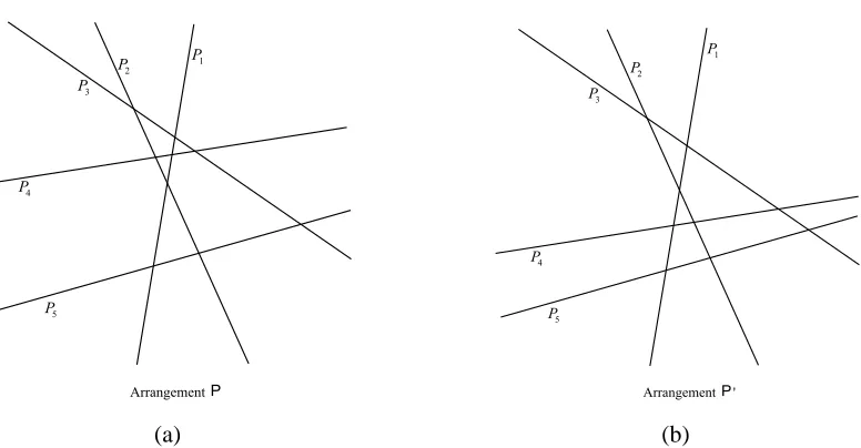
P1
P2
P3
P4
P5
P Arrangement
(a)
P1
P2
P3
P4
P5
P Arrangement '
(b)
Figure 1: (a) An example linear-hyperplane arrangement
P
and (b) the result of a Pachner move of hyperplane P4onP
.the boundary of the 3- or 4-cube, as a 2- or 3-dimensional cubical structure on the 2- or 3-sphere respectively.
To better understand this move, consider the cubical face structure of the boundary V of the (d+1)-cube. This is a d-sphere containing 2d+2 cubes, each of dimension d. There are many embeddings of the(d−1)-sphere as a cubical subcomplex into V , dividing it into a pair of d-balls. One ball is combinatorially identical to U and the other to U′.
There are a whole series of Pachner moves in each dimension d, but we are only interested in the ones where the pair of balls U,U′ have the same numbers of d-cubes. In Figure 1 a change in a hyperplane arrangement is shown, which corresponds to a Pachner move on the corresponding one-inclusion graph (considered as a cubical complex).
2.3 Concept Classes and their Learnability
A concept class C on domain X , is a subset of the power set of set X or equivalently C⊆ {0,1}X. We
primarily consider finite domains and so will write C⊆ {0,1}nin the sequel, where it is understood
that n=|X|and the n dimensions or colors are identified with an ordering{xi}ni=1=X .
The one-inclusion graph
G
(C)of C⊆ {0,1}n is the graph with vertex-set C and edge-setcon-taining{u,v} ⊆C iff u and v differ on exactly one component (Haussler et al., 1994);
G
(C)forms the basis of a prediction strategy with essentially-optimal worst-case expected risk.G
(C) can be viewed as a simplicial complex inRnby filling in each face with a product of continuous intervals (Rubinstein et al., 2009). Each edge{u,v}inG
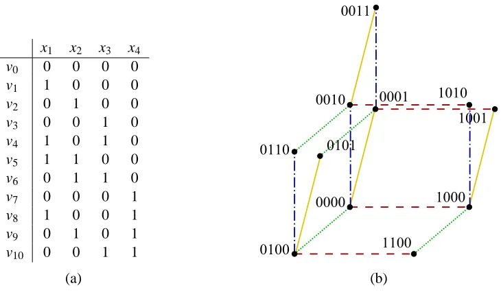
(C)is labeled by the component on which the two vertices u,v differ.Example 1 An example concept class in{0,1}4is enumerated in Figure 2(a). The corresponding
x1 x2 x3 x4
v0 0 0 0 0
v1 1 0 0 0
v2 0 1 0 0
v3 0 0 1 0
v4 1 0 1 0
v5 1 1 0 0
v6 0 1 1 0
v7 0 0 0 1
v8 1 0 0 1
v9 0 1 0 1
v10 0 0 1 1
(a) 0011 0010 0110 0100 1100 1000 1010 1001 0001 0000 0101 (b)
Figure 2: (a) A concept class in{0,1}4that is maximum with VC-dim 2 and (b) the one-inclusion
graph of the concept class.
the object as a simplicial complex: in this case the concepts form vertices which are connected by edges; these edges bound 2-cubes.
Probably Approximately Correct learnability of a concept class C⊆ {0,1}X is characterized by
the finiteness of the Vapnik-Chervonenkis (VC) dimension of C (Blumer et al., 1989). One key to all such results is Sauer’s Lemma.
Definition 7 The VC dimension of concept class C ⊆ {0,1}X is defined as VC(C) =
supnn ∃Y ∈
X n
,ΠY(C) ={0,1}n
o
where ΠY(C) ={(c(x1), . . . ,c(xn))|c∈C} ⊆ {0,1}n is the
projection of C on sequence Y= (x1, . . . ,xn).
Lemma 8 (Vapnik and Chervonenkis, 1971; Sauer, 1972; Shelah, 1972) The cardinality of any
concept classes C⊆ {0,1}nis bounded by|C| ≤∑VC(C) i=1
n i
.
Motivated by maximizing concept class cardinality under a fixed VC dimension, which is related to constructing general sample compression schemes (see Section 2.4), Welzl (1987) defined the following special classes.
Definition 9 Concept class C⊆ {0,1}X is called maximal if VC(C∪ {c})>VC(C) for all c∈ {0,1}X\C. Furthermore ifΠ
Y(C)satisfies Sauer’s Lemma with equality for each Y∈ Xn
, for every n∈N, then C is termed maximum. If C⊆ {0,1}n then C is maximum (and hence maximal) if C meets Sauer’s Lemma with equality.
Example 2 The concept class of Example 1 has VC-dimension 2 as witnessed by projecting onto
001
011
010 110
100 101
000
(a)
001
010
100 000
(b)
0110
1100 1010
(c)
Figure 3: The (a) projection (b) reduction and (c) tail of the concept class of Figure 2 with respect to projecting on to the first three coordinates (i.e., projecting out the fourth coordinate).
The reduction of C ⊆ {0,1}n with respect to i ∈ [n] = {1, . . . ,n} is the class Ci = Π[n]\{i}
c∈C|i∈IG(C)(c) where IG(C)(c)⊆[n]denotes the labels of the edges incident to vertex c; a multiple reduction is the result of performing several reductions in sequence. The tail of class C is taili(C) =
c∈C|i∈/IG(C)(c) . Welzl showed that if C is d-maximum, thenΠ[n]\{i}(C)and Ci
are maximum of VC-dimensions d and d−1 respectively.
Example 3 A projection, reduction and tail of the concept class of Figure 2 are shown in
Fig-ures 3(a)—3(c) respectively, when projecting onto coordinates{1,2,3}. In particular note that the reduction, like the projection, is a class in the smaller 3-cube while the tail is in the original 4-cube. Moreover note that the projection and reduction and maximum with VC-dimensions 2 and 1 respectively.
The results presented below relate to other geometric and topological representations of maxi-mum classes existing in the literature. Under the guise of ‘forbidden labels’, Floyd (1989) showed that maximum C⊆ {0,1}n of VC-dim d is the union of a maximally overlapping d-complete
col-lection of cubes (Rubinstein et al., 2009)—defined as a colcol-lection of(nd) d-cubes which uniquely project onto all(dn)possible sets of d coordinate directions. (An alternative proof was developed by Neylon 2006.) It has long been known that VC-1 maximum classes have one-inclusion graphs that are trees (Dudley, 1985); we previously extended this result by showing that when viewed as com-plexes, d-maximum classes are contractible d-cubical complexes (Rubinstein et al., 2009). Finally the cells of a simple linear arrangement of n hyperplanes inRd form a VC-d maximum class in the n-cube (Edelsbrunner, 1987), but not all finite maximum classes correspond to such Euclidean arrangements (Floyd, 1989).
Example 4 It is immediately clear from visual inspection that the 2-maximum concept classes of
Figures 2 and 3(a) are composed of complete collections of 2-cubes. Similarly the 1-maximum class of Figure 3(c) is a tree with one edge of each color.
2.4 Sample Compression Schemes
is only known that maximum classes can be d-compressed (Floyd, 1989). Unlabeled compression was first explored by Ben-David and Litman (1998); Kuzmin and Warmuth (2007) defined unla-beled compression as follows, and explicitly constructed schemes of size d for maximum classes.
Definition 10 Let C be a d-maximum class on a finite domain X . A mapping r is called a
represen-tation mapping of C if it satisfies the following conditions:
1. r is a bijection between C and subsets of X of size at most d; and
2. [non-clashing] :2 Πr(c)∪r(c′)(c)6=Πr(c)∪r(c′)(c′)for all c,c′∈C, c6=c′.
As with all previously published labeled schemes, all previously known unlabeled compression schemes for maximum classes exploit their special recursive projection-reduction structure and so it is doubtful that such schemes will generalize. Kuzmin and Warmuth (2007, Conjecture 2) conjec-tured that their min-peeling algorithm constitutes an unlabeled d-compression scheme for maximum classes; it iteratively removes minimum degree vertices from
G
(C), representing the corresponding concepts by the remaining incident dimensions in the graph. The authors also conjectured that sweeping a hyperplane in general position across a simple linear arrangement forms a compres-sion scheme that corresponds to min peeling the associated maximum class (Kuzmin and Warmuth, 2007, Conjecture 1). A particularly promising approach to compressing general classes is via their maximum-embeddings: a class C embedded in class C′ trivially inherits any compression scheme for C′, and so an important open problem is to embed maximal classes into maximum classes with at most a linear increase in VC dimension (Kuzmin and Warmuth, 2007, Open Problem 3).3. Preliminaries
A first step towards characterizing and compressing maximum classes is a process of building them. After describing this process of lifting we discuss compressing maximum classes by peeling, and properties of the boundaries of maximum classes.
3.1 Constructing All Maximum Classes
The aim in this section is to describe an algorithm for constructing all maximum classes of VC-dimension d in the n-cube. This process can be viewed as the inverse of mapping a maximum class to its d-maximum projection on[n]\{i}and the corresponding(d−1)-maximum reduction.
Definition 11 Let C,C′⊆ {0,1}n be maximum classes of VC-dimensions d,d−1 respectively, so
that C′⊂C, and let C1,C2⊂C be d-cubes, that is, d-faces of the n-cube{0,1}n.
1. C1,C2are connected if there exists a path in the one-inclusion graph
G
(C)with end-points in C1and C2; and
2. C1,C2 are said to be C′-connected if there exists such a connecting path that further does not
intersect C′.
The C′-connected components of C are the equivalence classes of the d-cubes of C under the C′ -connectedness relation.
Algorithm 1 MAXIMUMCLASSES(n,d) Given: n∈N,d∈[n]
Returns: the set of d-maximum classes in{0,1}n 1. if d=0 then return{{v} |v∈ {0,1}n} ; 2. if d=n then return{0,1}n ;
3.
M
← /0 ;for each C∈MAXIMUMCLASSES(n−1,d),
C′∈MAXIMUMCLASSES(n−1,d−1)s.t. C′⊂C do
4. {C1, . . . ,Ck} ←C′-connected components of C ; 5.
M
←M
∪Sp∈{0,1}kn
(C′× {0,1})∪Sq∈[k]Cq× {pq}
o ;
done 6. return
M
;The recursive algorithm for constructing all maximum classes of VC-dimension d in the n-cube, detailed as Algorithm 1, considers each possible d-maximum class C in the(n−1)-cube and each possible(d−1)-maximum subclass C′ of C as the projection and reduction of a d-maximum class
in the n-cube, respectively. The algorithm lifts C and C′ to all possible maximum classes in the n-cube. Then C′× {0,1}is contained in each lifted class; so all that remains is to find the tails from the complement of the reduction in the projection. It turns out that each C′-connected component Ci of C can be lifted to either Ci× {0} or Ci× {1}arbitrarily and independently of how the other
C′-connected components are lifted. The set of lifts equates to the set of d-maximum classes in the n-cube that project-reduce to(C,C′).
Lemma 12 MAXIMUMCLASSES(n,d)(cf. Algorithm 1) returns the set of maximum classes of
VC-dimension d in the n-cube for all n∈N,d∈[n].
Proof We proceed by induction on n and d. The base cases correspond to n∈N,d∈ {0,n}for which all maximum classes, enumerated as singletons in the n-cube and the n-cube itself respectively, are correctly produced by the algorithm. For the inductive step we assume that for n∈N,d∈[n−1]all maximum classes of VC-dimension d and d−1 in the(n−1)-cube are already known by recursive calls to the algorithm. Given this, we will show that MAXIMUMCLASSES(n,d) returns only d-maximum classes in the n-cube, and that all such classes are produced by the algorithm.
Let classes C∈MAXIMUMCLASSES(n−1,d)and C′∈MAXIMUMCLASSES(n−1,d−1)be
such that C′⊂C. Then C is the union of a d-complete collection and C′is the union of a(d− 1)-complete collection of cubes that are faces of the cubes of C. Consider a concept class C⋆ formed from C and C′by Algorithm 1. The algorithm partitions C into C′-connected components C1, . . . ,Ck
each of which is a union of d-cubes. While C′is lifted to C′× {0,1}, some subset of the components
{Ci}i∈S0 are lifted to{Ci× {0}}i∈S0 while the remaining components are lifted to {Ci× {1}}i∈/S0. Here S0ranges over all subsets of[k], selecting which components are lifted to 0; the complement
of S0 specifies those components lifted to 1. By definition C⋆ is a d-complete collection of cubes
with cardinality equal to (≤nd) since|C⋆|=|C′|+|C|(Kuzmin and Warmuth, 2007). So C⋆ is
d-maximum (Rubinstein et al., 2009, Theorem 34).
If we now consider any d-maximum class C⋆⊆ {0,1}n, its projection on[n]\{i}is a d-maximum
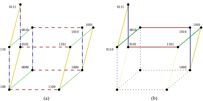
0011
0010
0110
0100 1100
1000 1011
1001 0001
0000 0101
(a)
0011
0010
0110
0100
1101
1000 1011
1001 0001
0000 0101
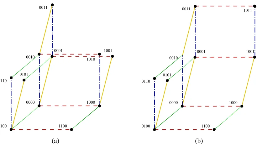
(b)
Figure 4: 2-maximum concept classes in{0,1}4constructed by lifting concept class Figure 3(a) as
the projection, and concept class Figure 3(b) as the reduction.
which contain color i. It is thus clear that C⋆ must be obtained by lifting parts of the C′-connected components of C to the 1 level and the remainder to the 0 level, and C′to C′× {0,1}. We will now show that if the vertices of each component are not lifted to the same levels, then while the number of vertices in the lift match that of a d-maximum class in the n-cube, the number of edges are too few for such a maximum class. Define a lifting operator on C asℓ(v) ={v} ×ℓv, whereℓv⊆ {0,1}
and
|ℓv| = (
2 , if v∈C′
1, if v∈C\C′ .
Consider now an edge {u,v} in
G
(C). By the definition of a C′-connected component thereex-ists some Cj such that either u,v∈Cj\C′, u,v∈C′ or WLOG u∈Cj\C′,v∈C′. In the first case ℓ(u)∪ℓ(v) is an edge in the lifted graph iff ℓu=ℓv. In the second case ℓ(u)∪ℓ(v) contains four
edges and in the last it contains a single edge. Furthermore, it is clear that this accounts for all edges in the lifted graph by considering the projection of an edge in the lifted product. Thus any lift other than those produced by Algorithm 1 induces strictly too few edges for a d-maximum class in the n-cube (cf. Kuzmin and Warmuth, 2007, Corollary 7.5).
3.2 Corner Peeling
Kuzmin and Warmuth (2007, Conjecture 2) conjectured that their simple min-peeling procedure is a valid unlabeled compression scheme for maximum classes. Beginning with a concept class C0=C⊆ {0,1}n, min peeling operates by iteratively removing a vertex vt of minimum-degree
in
G
(Ct) to produce the peeled class Ct+1=Ct\{vt}. The concept class corresponding to vt isthen represented by the dimensions of the edges incident to vt in
G
(Ct), IG(Ct)(vt)⊆[n]. Providingthat no-clashing holds for the algorithm, the size of the min-peeling scheme is the largest degree encountered during peeling. Kuzmin and Warmuth predicted that this size is always at most d for d-maximum classes. We explore these questions for a related special case of peeling, where we prescribe which vertex to peel at step t as follows.
Definition 13 We say that C⊆ {0,1}ncan be corner peeled if there exists an ordering v1, . . . ,v |C|
of the vertices of C such that, for each t∈[|C|]where C0=C,
1. vt∈Ct−1and Ct=Ct−1\{vt};
2. There exists a unique cube Ct′−1of maximum dimension over all cubes in Ct−1containing vt;
3. The neighborsΓ(vt)of vt in
G
(Ct−1)satisfyΓ(vt)⊆Ct′−1; and4. C|C|=/0.
The vt are termed the corner vertices of Ct−1respectively. If d is the maximum degree of each vt in
G
(Ct−1), then C is d corner peeled.Note that we do not constrain the cubes Ct′ to be of non-increasing dimension. It turns out that an important property of maximum classes is invariant to this kind of peeling.
Definition 14 We call a class C⊆ {0,1}nshortest-path closed if for any u,v∈C,
G
(C)contains apath connecting u,v of lengthku−vk1.
Lemma 15 If C⊆ {0,1}nis shortest-path closed and v∈C is a corner vertex of C, then C\{v}is
shortest-path closed.
Proof Consider a shortest-path closed C⊆ {0,1}n. Let c be a corner vertex of C, and denote the
cube of maximum dimension in C, containing c, by C′. Consider{u,v} ⊆C\{c}. By assumption there exists a u-v-path p of lengthku−vk1contained in C. If c is not in p then p is contained in the
peeled product C\{c}. If c is in p then p must cross C′ such that there is another path of the same length which avoids c, and thus C\{c}is shortest-path closed.
3.2.1 CORNERPEELINGIMPLIESCOMPRESSION
Theorem 16 If a maximum class C can be corner peeled then C can be d-unlabeled compressed. Proof The invariance of the shortest-path closed property under corner peeling is key. The
0000 1000 0010
1010
0100 1100
0110
0101
1001 0111
1101
(a)
1000 0010
1010
0110
0101
1001 0111
1101
(b)
Figure 5: (a) A 2-maximum class in the 4-cube and (b) its boundary highlighted by solid lines.
the cube Ct′−1 which is deleted from Ct−1 when vt is corner peeled. We claim that any two
ver-tices vs,vt ∈C have non-clashing representatives. WLOG, suppose that s<t. The class Cs−1must
contain a shortest vs-vt-path p. Let i be the color of the single edge contained in p that is incident
to vs. Color i appears once in p, and is contained in r(vs). This implies that vs,i 6=vt,i and that
i∈r(vs)∪r(vt), and so vs|(r(vs)∪r(vt))6=vt|(r(vs)∪r(vt)). By construction, r(·) is a bijection
between C and all subsets of[n]of cardinality≤VC(C).
If the oriented one-inclusion graph, with each edge directed away from the incident vertex rep-resented by the edge’s color, has no cycles, then that representation’s compression scheme is termed acyclic (Floyd, 1989; Ben-David and Litman, 1998; Kuzmin and Warmuth, 2007).
Proposition 17 All corner-peeling unlabeled compression schemes are acyclic.
Proof We follow the proof that the min-peeling algorithm is acyclic (Kuzmin and Warmuth, 2007).
Let v1, . . . ,v|C|be a corner vertex ordering of C. As a corner vertex vt is peeled, its unoriented
inci-dent edges are oriented away from vt. Thus all edges incident to v1are oriented away from v1and
so the vertex cannot take part in any cycle. For t>1 assume Vt ={vs|s<t}is disjoint from all
cycles. Then vt cannot be contained in a cycle, as all incoming edges into vt are incident to some
vertex in Vt. Thus the oriented
G
(C)is indeed acyclic.3.3 Boundaries of Maximum Classes
B,C A
A
C B
Figure 6: The first steps of building the dunce hat in Example 7.
Definition 18 The boundary ∂C of a d-maximum class C is defined as all the (d−1)-subcubes which are the faces of a single d-cube in C.
Maximum classes, when viewed as cubical complexes, are analogous to soap films (an example of a minimal energy surface encountered in nature), which are obtained when a wire frame is dipped into a soap solution. Under this analogy the boundary corresponds to the wire frame and the number of d-cubes can be considered the area of the soap film. An important property of the boundary of a maximum class is that all lifted reductions meet the boundary multiple times.
Theorem 19 Every d-maximum class has boundary containing at least two(d−1)-cubes of every combination of d−1 colors, for all d>1.
Proof We use the lifting construction of Section 3.1. Let C⋆⊆ {0,1}n be a 2-maximum class and
consider color i∈[n]. Then the reduction C⋆i is an unrooted tree with at least two leaves, each of which lifts to an i-colored edge in C⋆. Since the leaves are of degree 1 in C⋆i, the corresponding lifted edges belong to exactly one 2-cube in C⋆and so lie in∂C⋆. Consider now a d-maximum class C⋆⊆ {0,1}nfor d>2, and make the inductive assumption that the projection C=Π
[n−1](C⋆)has two of each type of(d−1)-cube, and that the reduction C′=C⋆nhas two of each type of(d− 2)-cube, in their boundaries. Pick d−1 colors I⊆[n]. If n∈I then consider two(d−2)-cubes colored by I\{xn}in∂C′. By the same argument as in the base case, these lift to two I-colored cubes in∂C⋆.
If n∈/I then∂C contains two I-colored(d−1)-cubes. For each cube, if the cube is contained in C′ then it has two lifts one of which is contained in∂C⋆, otherwise its unique lift is contained in∂C⋆. Therefore∂C⋆contains at least two I-colored cubes.
Example 6 The one-inclusion graph of a 2-maximum concept class in the 4-cube is depicted in
Fig-ure 5(a), along with its boundary of edges in FigFig-ure 5(b). Note that all four colors are represented by exactly two boundary edges in this case.
Example 7 Take a 2-simplex with vertices A,B,C. Glue the edges AB to AC to form a cone. Next glue the end loop BC to the edge AB . The result is a complex D with a single vertex, edge and 2-simplex, which is classically known as the dunce hat (cf. Figure 6). It is not hard to verify that D is contractible, but has no (geometric) boundary.
Although Theorem 19 will not be explicitly used in the sequel, we return to boundaries of maximum complexes later.
4. Euclidean Arrangements
Definition 20 A linear arrangement is a collection of n≥d oriented hyperplanes inRd. Each region or cell in the complement of the arrangement is naturally associated with a concept in{0,1}n; the
side of the ith hyperplane on which a cell falls determines the concept’s ith component. A simple
arrangement is a linear arrangement in which any subset of d planes has a unique point in common and all subsets of d+1 planes have an empty mutual intersection. Moreover any subset of k<d planes meet in a plane of dimension d−k. Such a collection of n planes is also said to be in general position.
Many of the familiar operations on concept classes in the n-cube have elegant analogues on arrangements.
• Projection on[n]\{i}corresponds to removing the ithplane;
• The reduction Ci is the new arrangement given by the intersection of C’s arrangement with the ithplane; and
• The corresponding lifted reduction is the collection of cells in the arrangement that adjoin the ith plane.
A k-cube in the one-inclusion graph corresponds to a collection of 2k cells, all having a common
(d−k)-face, which is contained in the intersection of k planes, and an edge corresponds to a pair of cells which have a common face on a single plane. The following result is due to Edelsbrunner (1987).
Lemma 21 The concept class C⊆ {0,1}n induced by a simple linear arrangement of n planes in
Rdis d-maximum.
Proof Note that C has VC dimension at most d, since general position is invariant to projection, that
is, no d+1 planes are shattered. Since C is the union of a d-complete collection of cubes (every cell contains d-intersection points in its boundary) it follows that C is d-maximum (Rubinstein et al., 2009).
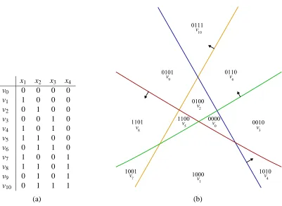
x1 x2 x3 x4
v0 0 0 0 0
v1 1 0 0 0
v2 0 1 0 0
v3 0 0 1 0
v4 1 0 1 0
v5 1 1 0 0
v6 0 1 1 0
v7 1 0 0 1
v8 1 1 0 1
v9 0 1 0 1
v10 0 1 1 1
(a) 0000 1100 0100 0111 0101 0110 1101 0010 1000 1001 1010 v
8 v3
v 0 v 5 v 2 v 6 v 9 v 10 v 1 v
7 v4
(b)
Figure 7: (a) The enumeration of the 2-maximum class in{0,1}4in Figure 5(a) and (b) a simple
linear line arrangement corresponding to the class, with each cell corresponding to a unique vertex.
Corollary 22 Let A be a simple linear arrangement of n hyperplanes in Rd with corresponding
d-maximum C⊆ {0,1}n. The intersection of A with a generic hyperplane corresponds to a(d−
1)-maximum class C′⊆C. In particular if all d-intersection points of A lie to one side of the generic hyperplane, then C′lies on the boundary of C; and∂C is the disjoint union of two(d−1)-maximum sub-classes.
Proof The intersection of A with a generic hyperplane is again a simple arrangement of n
hyper-planes but now inRd−1. Hence by Lemma 21 C′is a(d−1)-maximum class in the n-cube. C′⊆C
since the adjacency relationships on the cells of the intersection are inherited from those of A. Suppose that all d-intersections in A lie in one half-space of the generic hyperplane. C′ is the union of a(d−1)-complete collection. We claim that each of these(d−1)-cubes is a face of exactly one d-cube in C and is thus in∂C. A(d−1)-cube in C′corresponds to a line in A where d−1 planes mutually intersect. The(d−1)-cube is a face of a d-cube in C iff this line is further intersected by a dth plane. This occurs for exactly one plane, which is closest to the generic hyperplane along this intersection line. For once the d-intersection point is reached, when following along the line away from the generic plane, a new cell is entered. This verifies the second part of the result.
Consider two parallel generic hyperplanes h1,h2 such that all d-intersection points of A lie in
in-duced by the intersection of A with h1and A with h2. Consider an arbitrary(d−1)-cube in∂C. As
before this cube corresponds to a region of a line formed by a mutual intersection of d−1 planes. Moreover this region is a ray, with one end-point at a d-intersection. Because the ray begins at a point between the generic hyperplanes h1,h2, it follows that the ray must cross exactly one of these.
Example 9 To illustrate, consider the 2-maximum class in Figure 5(a) that corresponds to the
simple linear arrangement in Figure 7(b). The boundary, shown in Figure 5(b) is clearly a disjoint union of two 1-maximum classes—in this case sticks.
Corollary 23 Let A be a simple linear arrangement of n hyperplanes inRd and let C⊆ {0,1}n be
the corresponding d-maximum class. Then C considered as a cubical complex is homeomorphic to the d-ball Bd; and ∂C considered as a(d−1)-cubical complex is homeomorphic to the(d− 1)-sphere Sd−1.
Proof We construct a Voronoi cell decomposition corresponding to the set of d-intersection points
inside a very large ball in Euclidean space. By induction on d, we claim that this is a cubical complex and the vertices and edges correspond to the class C. By induction, on each hyperplane, the induced arrangement has a Voronoi cell decomposition which is a(d−1)-cubical complex with edges and vertices matching the one-inclusion graph for the tail of C corresponding to the label associated with the hyperplane. It is not hard to see that the Voronoi cell defined by a d-intersection point p on this hyperplane is a d-cube. In fact, its (d−1)-faces correspond to the Voronoi cells for p, on each of the d hyperplanes passing through p. We also see that this d-cube has a single vertex in the interior of each of the 2d cells of the arrangement adjacent to p. In this way, it follows that the vertices of this Voronoi cell decomposition are in bijective correspondence to the cells of the hyperplane arrangement. Finally the edges of the Voronoi cells pass through the faces in the hyperplanes. So these correspond bijectively to the edges of C, as there is one edge for each face of the hyperplanes. Using a very large ball, containing all the d-intersection points, the boundary faces become spherical cells. In fact, these form a spherical Voronoi cell decomposition, so it is easy to replace these by linear ones by taking the convex hull of their vertices. So a piecewise linear cubical complex C is constructed, which has one-skeleton (graph consisting of all vertices and edges) isomorphic to the one-inclusion graph for C.
Finally we want to prove that C is homeomorphic to Bd. This is quite easy by construction. For
we see that C is obtained by dividing up Bdinto Voronoi cells and replacing the spherical boundary cells by linear ones, using convex hulls of the boundary vertices. This process is clearly given by a homeomorphism by projection. In fact, the homeomorphism preserves the PL-structure so is a PL homeomorphism.
Example 10 Consider again the one-inclusion graph in Figure 5(a) corresponding to a 2-maximum
0000 1100
0100 0111
0101 0110
1101 0010
1000
1001 1010
v
8 v3
v
0
v
5
v
2
v
6
v
9
v
10
v
1
v
7 v4
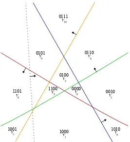
Figure 8: The simple linear line arrangement from Figure 7(b) corresponding to the concept class enumerated in Figure 7(a) and visualized in Figure 5(a). The arrangement is in the process of being swept by the dashed line.
The following example demonstrates that not all maximum classes of VC-dimension d are homeomorphic to the d-ball. The key to such examples is branching.
Example 11 A simple linear arrangement inRcorresponds to points on the line—cells are simply intervals between these points and so corresponding 1-maximum classes are sticks. Any tree that is not a stick can therefore not be represented as a simple linear arrangement inRand is also not homeomorphic to the 1-ball which is simply the interval[−1,1].
As Kuzmin and Warmuth (2007) did previously, consider a generic hyperplane h sweeping across a simple linear arrangement A. h begins with all d-intersection points of A lying in its positive half-space
H
+. The concept corresponding to cell c is peeled from C when|H
+∩c|=1, that is, h crosses the last d-intersection point adjoining c. At any step in the process, the result of peeling j vertices from C to reach Cj, is captured by the arrangementH
+∩A for the appropriate h.Example 12 Figure 7(a) enumerates the 11 vertices of a 2-maximum class in the 4-cube. Figures 8
and 5(a) display a hyperplane arrangement in Euclidean space and its Voronoi cell decomposition, corresponding to this maximum class. In this case, sweeping the vertical dashed line across the arrangement corresponds to a partial corner peeling of the concept class with peeling sequence v7,
Next we resolve the first half of Kuzmin and Warmuth (2007, Conjecture 1).
Theorem 24 Any d-maximum class C⊆ {0,1}n corresponding to a simple linear arrangement A
can be corner peeled by sweeping A, and this process is a valid unlabeled compression scheme for C of size d.
Proof We must show that as the jthd-intersection point pjis crossed, there is a corner vertex of Cj−1
peeled away. It then follows that sweeping a generic hyperplane h across A corresponds to corner peeling C to a(d−1)-maximum sub-class C′⊆∂C by Corollary 22. Moreover C′ corresponds to a simple linear arrangement of n hyperplanes inRd−1.
We proceed by induction on d, noting that for d=1 corner peeling is trivial. Consider h as it approaches the jthd-intersection point pj. The d planes defining this point intersect h in a simple
arrangement of hyperplanes on h. There is a compact cell ∆ for the arrangement on h, which is a d-simplex3 and shrinks to a point as h passes through pj. We claim that the cell c for the
arrangement A, whose intersection with h is∆, is a corner vertex vj of Cj−1. Consider the lines
formed by intersections of d−1 of the d hyperplanes, passing through pj. Each is a segment
starting at pj and ending at h without passing through any other d-intersection points. So all faces
of hyperplanes adjacent to c meet h in faces of∆. Thus, there are no edges in Cj−1starting at the
vertex corresponding to pj, except for those in the cube C′j−1, which consists of all cells adjacent to
pj in the arrangement A. So c corresponds to a corner vertex vj of the d-cube C′j−1in Cj−1. Finally,
just after the simplex is a point, c is no longer in
H
+and so vj is corner peeled from Cj−1.Theorem 16 completes the proof that this corner peeling of C constitutes unlabeled compres-sion.
Corollary 25 The sequence of cubes C0′, . . . ,C|′C|, removed when corner peeling by sweeping simple linear arrangements, is of non-increasing dimension. In fact, there are nd cubes of dimension d, then d−n1
cubes of dimension d−1, etc.
While corner peeling and min peeling share some properties in common, they are distinct proce-dures. Notice that sweeping produces a monotonic corner-peeling sequence, as cubes are removed in order of non-increasing dimensions.
Example 13 Consider sweeping a simple linear arrangement corresponding to a 2-maximum class.
After all but one 2-intersection point has been swept, the corresponding corner-peeled class Ct is
the union of a single 2-cube with a 1-maximum stick. Min peeling applied to Ct would first peel a
leaf, while sweeping must peel the 2-cube next.
A second example is the class in a 3-cube which consists of six vertices, so that two opposite vertices, for example, 000 and 111 are not included. This class cannot be corner peeled as the one-inclusion graph consists of six edges forming a single cycle. On the other hand, it has many min-peeling schemes.
An interesting question is if a class has a corner-peeling scheme, does it always have a min-peeling scheme which is also a corner-min-peeling scheme? This is given as Question 50 below.
The next result follows from our counter-examples to Kuzmin & Warmuth’s minimum degree conjecture (Rubinstein et al., 2009).
Corollary 26 There is no constant c so that all maximal classes of VC-dimension d can be
embed-ded into maximum classes corresponding to simple hyperplane arrangements of dimension d+c.
5. Hyperbolic Arrangements
To motivate the introduction of hyperbolic arrangements, note that linear-hyperplane arrangements can be efficiently described, since each hyperplane is determined by its unit normal and distance from the origin. Similarly, a hyperbolic hyperplane is a hypersphere. So it can be parametrized by its center—a point on the ideal sphere at infinity—and its radius.4
However the family of hyperbolic hyperplanes has more flexibility than linear hyperplanes since there are many disjoint hyperbolic hyperplanes, whereas in the linear case only parallel hyperplanes do not meet. Thus we turn to hyperbolic arrangements to represent a larger collection of concept classes than those represented by simple linear arrangements.
We briefly discuss the Klein model of hyperbolic geometry (Ratcliffe, 1994, pg. 7). Consider the open unit ball Hk in Rk. Geodesics (lines of shortest length in the geometry) are given by intersections of straight lines inRkwith the unit ball. Similarly planes of any dimension between 2
and k−1 are given by intersections of such planes inRk with the unit ball. Note that such planes are completely determined by their spheres of intersection with the unit sphere Sk−1, which is called the ideal boundary of hyperbolic spaceHk. Note that in the appropriate metric, the ideal boundary
consists of points which are infinitely far from all points in the interior of the unit ball.
We can now see immediately that a simple hyperplane arrangement inHk can be described by taking a simple hyperplane arrangement inRk and intersecting it with the unit ball. However we require an important additional property to mimic the Euclidean case. Namely we add the constraint that every subcollection of d of the hyperplanes inHk has mutual intersection points insideHk, and that no(d+1)-intersection point lies in Hk. We need this requirement to obtain that the resulting class is maximum.
Definition 27 A simple hyperbolic d-arrangement is a collection of n hyperplanes inHk with the property that every sub-collection of d hyperplanes mutually intersect in a (k−d)-dimensional hyperbolic plane, and that every sub-collection of d+1 hyperplanes mutually intersect as the empty set.
Corollary 28 The concept class C corresponding to a simple d-arrangement of hyperbolic
hyper-planes inHk is d-maximum in the k-cube.
Proof The result follows by the same argument as before. Projection cannot shatter any(d+ 1)-cube and the class is a complete union of d-1)-cubes, so is d-maximum.
The key to why hyperbolic arrangements represent many new maximum classes is that they allow flexibility of choosing d and k independently. This is significant because the unit ball can be
chosen to miss much of the intersections of the hyperplanes in Euclidean space. Note that the new maximum classes are embedded in maximum classes induced by arrangements of linear hyperplanes in Euclidean space.
A simple example is any 1-maximum class. It is easy to see that this can be realized in the hyperbolic plane by choosing an appropriate family of lines and the unit ball in the appropriate po-sition. In fact, we can choose sets of pairs of points on the unit circle, which will be the intersections with our lines. So long as these pairs of points have the property that the smaller arcs of the circle between them are disjoint, the lines will not cross inside the disk and the desired 1-maximum class will be represented.
Corner-peeling maximum classes represented by hyperbolic-hyperplane arrangements proceeds by sweeping, just as in the Euclidean case. Note first that intersections of the hyperplanes of the arrangement with the moving hyperplane appear precisely when there is a first intersection at the ideal boundary. Thus it is necessary to slightly perturb the collection of hyperplanes to ensure that only one new intersection with the moving hyperplane occurs at any time. Note also that new intersections of the sweeping hyperplane with the various lower dimensional planes of intersection between the hyperplanes appear similarly at the ideal boundary. The important claim to check is that the intersection at the ideal boundary between the moving hyperplane and a lower dimensional plane, consisting entirely of d intersection points, corresponds to a corner-peeling move. We include two examples to illustrate the validity of this claim.
Example 14 In the case of a 1-maximum class coming from disjoint lines inH2, a cell can disap-pear when the sweeping hyperplane meets a line at an ideal point. This cell is indeed a vertex of the tree, that is, a corner-vertex.
Example 15 Assume that we have a family of 2-planes in the unit 3-ball which meet in pairs in
single lines, but there are no triple points of intersection, corresponding to a 2-maximum class. A corner-peeling move occurs when a region bounded by two half disks and an interval disappears, in the positive half space bounded by the sweeping hyperplane. Such a region can be visualized by taking a slice out of an orange. Note that the final point of contact between the hyperplane and the region is at the end of a line of intersection between two planes on the ideal boundary.
We next observe that sweeping by generic hyperbolic hyperplanes induces corner peeling of the corresponding maximum class, extending Theorem 24. As the generic hyperplane sweeps across hyperbolic space, not only do swept cells correspond to corners of d-cubes but also to corners of lower dimensional cubes as well. Moreover, the order of the dimensions of the cubes which are corner peeled can be arbitrary—lower dimensional cubes may be corner peeled before all the higher dimensional cubes are corner peeled. This is in contrast to Euclidean sweepouts (cf. Corollary 25). Similar to Euclidean sweepouts, hyperbolic sweepouts correspond to corner peeling and not min peeling.
Theorem 29 Any d-maximum class C⊆ {0,1}ncorresponding to a simple hyperbolic d-arrangement
A can be corner peeled by sweeping A with a generic hyperbolic hyperplane.
Proof We follow the same strategy of the proof of Theorem 24. For sweeping in hyperbolic space
0000 1000 0010
1010
0100 1100
0110
0101
0001 0011
1001
(a)
0000 1000
0010
1011
0100 1100
0110
0101
0001 0011
1001
(b)
Figure 9: 2-maximum classes in{0,1}4that can be represented as hyperbolic arrangements but not
as Euclidean arrangements.
the ideal boundary. Each d-cube C′ in C still corresponds to the cells adjacent to the intersection IC′ of d hyperplanes. But now IC′ is a (k−d)-dimensional hyperbolic hyperplane. A cell c adjacent to IC′ is corner peeled precisely when h last intersects c at a point of IC′ at the ideal boundary. As for simple linear arrangements, the general position of A∪ {h}ensures that corner-peeling events never occur simultaneously. For the case k=d+1, as for the simple linear arrangements just prior to the corner peeling of c,
H
+∩c is homeomorphic to a(d+1)-simplex with a missing face on the ideal boundary. And so as in the simple linear case, this d-intersection point corresponds to a corner d-cube. In the case k>d+1,H
+∩c becomes a(d+1)-simplex (as before) multiplied byRk−d−1. If k=d, then the main difference is just before corner peeling of c,H
+∩c is homeomorphic to a k-simplex which may be either closed (hence in the interior ofHk) or with a missing face on the ideal boundary. The rest of the argument remains the same, except for one important observation.Although swept corners in hyperbolic arrangements can be of cubes of differing dimensions, these dimensions never exceed d and so the proof that sweeping simple linear arrangements induces d-compression schemes is still valid.
Example 16 Constructed with lifting, Figure 9 completes the enumeration, up to symmetry, of the
2-maximum classes in{0,1}4begun with Example 12. These cases cannot be represented as simple
(a) (b)
Figure 10: Hyperbolic-hyperplane arrangements corresponding to the classes in Figure 9. In both cases the four hyperbolic planes meet in 6 straight line segments (not shown). The planes’ colors correspond to the edges’ colors in Figure 9.
Corollary 30 There is no constant c so that all maximal classes of VC-dimension d can be
em-bedded into maximum classes corresponding to simple hyperbolic-hyperplane arrangements of VC-dimension d+c.
This result follows from our counter-examples to Kuzmin & Warmuth’s minimum degree con-jecture (Rubinstein et al., 2009).
Corollary 28 gives a proper superset of simple linear-hyperplane arrangement-induced maxi-mum classes as hyperbolic arrangements. We will prove in Section 7 that all maximaxi-mum classes can be represented as PL-hyperplane arrangements in a ball. These are the topological analogue of hyperbolic-hyperplane arrangements. If the boundary of the ball is removed, then we obtain an arrangement of PL hyperplanes in Euclidean space.
6. Infinite Euclidean and Hyperbolic Arrangements
We consider a simple example of an infinite maximum class which admits corner peeling and a compression scheme analogous to those of previous sections.
Example 17 Let
L
be the set of lines in the plane of the form L2m={(x,y)|x=m}and L2n+1= {(x,y)|y=n}for m,n∈N. Let v00, v0n, vm0, and vmnbe the cells bounded by the lines{L2,L3},{L2,L2n+1,L2n+3},{L2m,L2m+2,L3}, and{L2m,L2m+2,L2n+1,L2n+3}, respectively. Then the cubical
complex C, with vertices vmn, can be corner peeled and hence compressed, using a sweepout by the
v
1
v
2
v
3
v
4
initialized sweeping hyperplane
(a)
v1
2-cube v 4
1-cube
v 3
2-cube v 2
2-cube
(b)
Figure 11: (a) The simple hyperbolic arrangement corresponding to the 2-maximum class in{0,1}4
of Figure 9(a)—as shown in Figure 10(a)—with a generic sweeping hyperplane shown in several positions before and after it sweeps past four cells; and (b) the class with the first four corner-vertices peeled by the hyperbolic arrangement sweeping. Notice that three 2-cubes are peeled, then a 1-cube (all shown) followed by 2-cubes.
To verify the properties of this example, notice that sweeping as specified corresponds to corner peeling the vertex v00, then the vertices v10,v01, then the remaining vertices vmn. The lines x+ (1+ ε)y=t are generic as they pass through only one intersection point of
L
at a time. Additionally, representing v00 by /0, v0n by {L2n+1}, vm0 by{L2m} and vmn by {L2m,L2n+1}constitutes a validunlabeled compression scheme. Note that the compression scheme is associated with sweeping across the arrangement in the direction of decreasing t. This is necessary to pick up the boundary vertices of C last in the sweepout process, so that they have either singleton representatives or the empty set. In this way, similar to Kuzmin and Warmuth (2007), we obtain a compression scheme so that every labeled sample of size 2 is associated with a unique concept in C, which is consistent with the sample. On the other hand to obtain corner peeling, we need the sweepout to proceed with t increasing so that we can begin at the boundary vertices of C.
In concluding this brief discussion, we note that many infinite collections of simple hyperbolic hyperplanes and Euclidean hyperplanes can also be corner peeled and compressed, even if inter-section points and cells accumulate. However a key requirement in the Euclidean case is that the concept class C has a non-empty boundary, when considered as a cubical complex. An easy ap-proach is to assume that all the d-intersections of the arrangement lie in a half-space. Moreover, since the boundary must also admit corner peeling, we require more conditions, similar to having all the intersection points lying in an octant.
Example 18 InR3, choose the family of planes
P
of the form P3n+i={x∈R3|xi+1=1−1/n}for
independent (in particular, no integral linear combination is rational) and α,β are both close to 1. This example has similar properties to Example 17: the compression scheme is again given by decreasing t whereas corner peeling corresponds to increasing t. Note that cells shrink to points, as x→1 and the volume of cells converge to zero as n→∞, or equivalently any xi→1.
Example 19 In the hyperbolic planeH2, represented as the unit circle centered at the origin inR2, choose the family of lines
L
given by L2n={(x,y)|x=1−1/n}and L2n+1={(x,y)|x+ny=1},for n≥1. This arrangement has corner peeling and compression schemes given by sweeping across
L
using the generic line{y=t}.7. Piecewise-Linear Arrangements
PL hyperplanes have the advantage that they can be easily manipulated, by cutting and pasting or isotoping part of a hyperplane to a new position, keeping the rest of the hyperplane fixed. How-ever a disadvantage is that there is no simple way of describing a PL hyperplane, similar to the parametrizations of either linear or hyperbolic hyperplanes. The methods of proof of our main re-sults about representing maximum classes and corner peeling, require PL-hyperplane arrangements. We conjecture that PL-hyperplane arrangements are equivalent to hyperbolic ones. This would give an interesting geometric approach of forming all maximum classes as simple hyperbolic arrange-ments.
A PL hyperplane is the image of a proper piecewise-linear homeomorphism from the(k− 1)-ball Bk−1 into Bk, that is, the inverse image of the boundary Sk−1 of the k-ball is Sk−2 (Rourke and Sanderson, 1982). A simple PL d-arrangement is an arrangement of n PL hyperplanes such that every subcollection of j hyperplanes meet transversely in a(k−j)-dimensional PL plane for 2≤ j≤d and every subcollection of d+1 hyperplanes are disjoint.
Corollary 31 The concept class C corresponding to a simple d-arrangement of PL hyperplanes in
Bkis d-maximum in the k-cube.
Proof The result follows by the same argument as in the linear or hyperbolic cases. Projection
cannot shatter any(d+1)-cube and the class is a complete union of d-cubes, so is d-maximum.
7.1 Maximum Classes are Represented by Simple PL-Hyperplane Arrangements
Our aim is to prove the following theorem by a series of steps.
Theorem 32 Every d-maximum class C⊆ {0,1}n can be represented by a simple arrangement of
PL hyperplanes in an n-ball. Moreover the corresponding simple arrangement of PL hyperspheres in the(n−1)-sphere also represents C, so long as n>d+1.
7.1.1 EMBEDDING Ad-MAXIMUMCUBICALCOMPLEX IN THEn-CUBE INTO ANn-BALL
We begin with a d-maximum cubical complex C⊆ {0,1}nembedded into[0,1]n. This gives a
nat-ural embedding of C intoRn. Take a small regular neighborhood
N
of C so that the boundary∂N
Figure 12: A 1-maximum class (thick solid lines) with its fattening (thin solid lines with points), bisecting sets (dashed lines) and induced complementary cells.
argument from topology due to Mazur 1961). Our aim is to prove that∂
N
is an(n−1)-sphere andN
is an n-ball. There are two ways of proving this: show that∂N
is simply connected and invoke the well-known solution to the generalized Poincar´e conjecture (Smale, 1961), or use the cubical structure of the n-cube and C to directly prove the result. We adopt the latter approach, al-though the former works fine. The advantage of the latter is that it produces the required hyperplane arrangement, not just the structures of∂N
andN
.7.1.2 BISECTINGSETS
For each color i, there is a hyperplane Pi inRn consisting of all vectors with ith coordinate equal
to 1/2. We can easily arrange the choice of regular neighborhood
N
of C so thatN
i =Pi∩N
is a regular neighborhood of C∩Pi in Pi. (We call
N
i a bisecting set as it intersects C along the‘center’ of the reduction in the ith coordinate direction, see Figure 12.) But then since C∩P i is a
cubical complex corresponding to the reduction Ci, by induction on n, we can assert that
N
i is an(n−1)-ball. Similarly the intersections
N
i∩N
j can be arranged to be regular neighborhoods of(d−2)-maximum classes and are also balls of dimension n−2, etc. In this way, we see that if we can show that
N
is an n-ball, then the induction step will be satisfied and we will have produced a PL-hyperplane arrangement (the system ofN
iinN
) in a ball.7.1.3 SHIFTING
To complete the induction step, we use the technique of shifting (Alon, 1983; Frankl, 1983; Haus-sler, 1995). In our situation, this can be viewed as the converse of lifting. Namely if a color i is chosen, then the cubical complex C has a lifted reduction C′ consisting of all d-cubes containing the ith color. By shifting, we can move down any of the lifted components, obtained by splitting C open along C′, from the level xi=1 to the level xi=0, to form a new cubical complex C⋆. We claim
that the regular neighborhood of C is a ball if and only if the same is true for C⋆. But this is quite straightforward, since the operation of shifting can be thought of as sliding components of C, split open along C′, continuously from level xi=1 to xi=0. So there is an isotopy of the attaching maps