Revised Loss Bounds for the Set Covering Machine and Sample-Compression Loss Bounds for Imbalanced Data

Revised Loss Bounds for the Set Covering Machine and

Sample-Compression Loss Bounds for Imbalanced Data

Zakria Hussain [email protected]

Centre for Computational Statistics and Machine Learning University College London

London, UK, WC1E 6BT

Franc¸ois Laviolette [email protected]

Mario Marchand [email protected]

D´epartment IFT-GLO Universit´e Laval

Qu´ebec, Canada, G1V 0A6

John Shawe-Taylor [email protected]

Centre for Computational Statistics and Machine Learning University College London

London, UK, WC1E 6BT

Spencer Charles Brubaker [email protected]

Matthew D. Mullin [email protected]

College of Computing

Georgia Institute of Technology Atlanta, Georgia, 30332

Editor: G´abor Lugosi

Abstract

Marchand and Shawe-Taylor (2002) have proposed a loss bound for the set covering machine that has the property to depend on the observed fraction of positive examples and on what the clas-sifier achieves on the positive training examples. We show that this loss bound is incorrect. We then propose a loss bound, valid for any sample-compression learning algorithm (including the set covering machine), that depends on the observed fraction of positive examples and on what the classifier achieves on them. We also compare numerically the loss bound proposed in this paper with the incorrect bound, the original SCM bound and a recently proposed loss bound of Marchand and Sokolova (2005) (which does not depend on the observed fraction of positive examples) and show that the latter loss bounds can be substantially larger than the new bound in the presence of imbalanced misclassifications.

Keywords: set covering machines, sample-compression, loss bounds

1. Introduction

the selection of classifiers with guarantees of good generalization is to require some type of parsi-mony in the form of the functions. Typically seeking parsimonious solutions reduces to an NP-hard optimization, but an algorithm that delivers a good approximation to the optimal solution using a greedy approach is the so-called set covering machine (SCM). This approach for producing very sparse classifiers having good generalization was proposed by Marchand and Shawe-Taylor (2001). A generalization error bound is an upper bound on the expected test set performance that holds with high probability over the (random) choice of the training set. There are three ways in which such a bound can assist a user of adaptive systems technology. Firstly, the existence of such a bound justifying the form of a learning algorithm gives confidence in its reliability. This is the primary role of SVM bounds in most applications. The second is to guide model selection through setting regularization and hyperparameters to optimize the bound. The third is to give to users as a measure of performance. Experiments with recent SVM bounds have begun to make progress with the second goal, but it is fair to say that the third goal is still to be realized.

The situation with SCM bounds is that they are typically tighter and more reliable than those derived for SVMs. The classifier output by the SCM is described by a small subset of the training data called the compression set. By adapting the pioneering work of Littlestone and Warmuth (1986) on sample-compression schemes, Marchand and Shawe-Taylor (2001) have been able to obtain a loss bound that depends on the size (i.e., the number of examples) of the compression set of the SCM classifier. More recently, Marchand and Sokolova (2005) have been able to obtain a tighter bound, which applies to any sample-compression learning algorithm (including the SCM), by making use of sample-compression-dependent sets of messages. None of these loss bounds, however, depend on the observed fraction of positive examples in the training set and on the fraction of positive examples used for the compression set of the final classifier. Consequently, these loss bounds are not appropriate for identifying classifiers that perform well under frequently encountered distributions where the examples of one class are much more abundant than the examples of the other class (the class imbalance case) or when the loss suffered by misclassifying a positive example differs greatly from the loss suffered by misclassifying a negative example (the asymmetrical loss case).

To obtain a loss bound that reflects more accurately the performance of classifiers trained on imbalanced data sets, Marchand and Shawe-Taylor (2002) have proposed a SCM loss bound that depends on the observed fraction of positive examples in the training set and on the fraction of positive examples used for the compression set of the final classifier. However, we will show in Section 3 that this bound is incorrect. We then propose, in Section 4, a loss bound which is valid for any sample-compression learning algorithm (including the SCM) and that depends on the ob-served fraction of positive examples and on what the classifier achieves on the positive training examples. The proof of this new loss bound turns out to be much more involved than all other sample-compression loss bounds that do not depend on the observed fraction of positive examples (as in Marchand and Sokolova, 2005). Finally, for the SCM case, we compare numerically the loss bound of Section 4 with the recently proposed loss bound of Marchand and Sokolova (2005) (which does not depend on the observed fraction of positive examples) and show that the latter loss bound can be substantially larger than the former in the presence of imbalanced misclassifications.

less frequent than the dominant class. An example is classification of news articles by topic, where classification of all documents as not relevant will give good performance if we do not impose a greater cost on the misclassification of a relevant document.

We begin our discussion with preliminary definitions and terminology that will be used through-out the remainder of this paper.

2. Preliminary Definitions

Let the input space X be a set of n-dimensional vectors ofRnand let x be a member of X . We define a feature as an arbitrary Boolean-valued function that maps X onto{0,1}.

Consider any set

H

={hi}|_iH₌₁| of Boolean-valued features hi. We will consider learning algo-rithms that are given any such set

H

and return a small subset

R

⊂

H

of features. Given that subset

R

, and an arbitrary input vector x, the output f(x)of the Set Covering Machine (SCM) is given by the conjunction

f(x) = ^ i∈R

hi(x).

The function f contains a conjunction of features hi that individually give outputs hi(x) of 0 or 1 to denote whether the input vector x belongs to class 0 or class 1, respectively. Therefore, the function f outputs 0 or 1 according to a conjunction of features hi. A positive example will be referred to as a

P

-example and a negative example as a

N

-example. Given a training set S=SP∪S_N

of examples, the set of positive training examples will be denoted by S_P and the set of negative training examples by S_N.

Any learning algorithm that constructs a conjunction (such as the one above) can be transformed into an algorithm constructing a disjunction just by exchanging the role of the positive and negative examples. Hence, simply by reassigning the set of negative training examples to the set of positive training examples (i.e., S_P ←S_N) and the set of positive training examples to the set of negative training examples (i.e., S_N ←S_P) we can transform the algorithm into one that constructs a dis-junction. However, for the remainder of the paper we will assume, without loss of generality, that the SCM always produces a conjunction.

In this paper, we consider the case where

H

is the set of data-dependent balls.

Definition 1 For each training example xi with label yi∈ {0,1} and (real-valued) radius ρ, we define feature hi,ρto be the following data-dependent ball centered on xi:

hi,ρ(x)def=hρ(x,xi) =

yi if d(x,xi)<ρ y_i otherwise,

where y_idenotes the Boolean complement of yiand d(x,x0)denotes the distance between x and x0. Training example xiwill be called the ball center of hi,ρ.

To determine the radiusρof ball hi,ρ, we will use another training example xj, called the ball border of hi,ρ, such thatρ=d(xj,xi).

training set which identifies a classifier (here a SCM). The function that maps arbitrary compression sets to classifiers is called the reconstruction function. We refine further these notions in Section 4. We adopt the PAC model where it is assumed that each example(x,y)is drawn independently at random according to a fixed (but unknown) distribution. In this paper, we consider the probabilities of events taken separately over the

P

-examples and the

N

-examples. We will therefore denote by

P{a(x,y)

(x,y)∈

P

}the probability that predicate a is true on a random draw of an example(x,y), given that this example is positive. Hence, the error probability of classifier f on

P

-examples and on

N

-examples, that we call respectively the expected

P

-loss and the expected

N

-loss, are given

by

erP(f) def= P{f(x)6=y(x,y)∈

P

}, er_N(f) def= P{f(x)6=y(x,y)∈

N

}.

Similarly, let ˆer_P(f,S)denote the number of examples in S_P misclassified by f and let ˆer_N(f,S)) denote the number of examples in S_N misclassified by f . Hence

ˆ

er_P(f,S) def= |{(x,y)∈S_P: f(x)6=y}|,

ˆ

er_N(f,S) def=

{(x,y)∈SN : f(x)6=y} .

Throughout this paper, the probability of occurrence of a positive example will be denoted by

p_P. Similarly, p_N will denote the probability of occurrence of a negative example. We will consider the general case where the loss lP of misclassifying a positive example can differ from the loss l_N of misclassifying a negative example. We will denote by A(S)the classifier returned by the learning algorithm A trained on a set S of examples. In this case, the expected lossE[l(A(S))]of classifier

A(S)is defined as

E[l(A(S))] def= lP·pP·erP[A(S)] + l_N ·p_N ·er_N[A(S)]. (1)

3. Incorrect Bound

The Theorem 5 of Marchand and Shawe-Taylor (2002) gives the following loss bound for the SCM with the symmetric loss case of l_P =l_N =1.

Given the above definitions, let A be any learning algorithm that builds a SCM with data-dependent balls with the constraint that the returned function A(S)always correctly classifies every example in the compression set. Then, with probability 1−δover all training sets S of m examples,

E[l(A(S))] ≤ 1−exp

− 1

m−cp−b−cn−kp−kn

ln B+ln 1

δ0

,

where

δ0 def

=

π2

6 −5

·((cp+1)(cn+1)(b+1)(kp+1)(kn+1))−2·δ,

B def=

mp cp

mp−cp b

mn cn

mp−cp−b kp

mn−cn kn

and where kp and kn are the number of misclassified positive and negative training examples by classifier A(S). Similarly, cpand cnare the number of positive and negative ball centers contained in classifier A(S)whereas b denotes the number of ball borders1 in classifier A(S). Finally mpand mndenote the number of positive and negative examples in training set S.

Let us take the B expression only and look more closely at the number of ways of choosing the errors on SP and S_N:

mp−cp−b kp

mn−cn kn

.

The bound on the expected loss given above will be small only if each factor is small. However, each factor can be small for a small number of training errors (desirable) or a large number of training errors (undesirable). In particular, the product of these two factors will be small for a small value of

kn(say, kn=0) and a large value of kp(say, kp=mp−cp−b). In this case, the denominator of the bound given above will become

m−cp−b−cn−kp−kn=mn−cn,

and will be large whenever mncn. Consequently, the bound given by Theorem 5 of Marchand and Shawe-Taylor (2002) will be small for classifiers having a small compression set and making a large number of errors on SP and a small number of errors on S_N. Clearly, this is incorrect as it implies a classifier with good generalization ability and so exposes an error in the proof. In order to derive a loss bound where the issue of imbalanced misclassifications can be handled, the errors for positive and negative examples must be bounded separately.

The error in the proof of Theorem 5 of Marchand and Shawe-Taylor (2002) occurs at the first equality used in their Equation 3. This equality is tantamount to writing that for any fixed classifier

f :

P

S∈

X

: ˆer(f,S) =0

|SP|=mp

= (1−er_P(f))mp_(1−er

N(f))mn×

m mp

pmp

P (1−pP)mn _(false),

where p_P denotes the probability of occurrence of a

P

-example. However this last equation is false since the probability on the left hand side is conditioned on the fact the|SP|=mp. Hence, we have instead

P

S∈

X

: ˆer(f,S) =0

|S_P|=mp

= (1−er_P)mp_(1−er

N)mn_.

4. Sample-Compression Loss Bounds for Imbalanced Data

Recall that X denotes the input space. Let

X

= (X× {0,1})m_{be the set of training sets of size m} with inputs from X . We consider any learning algorithm A having the property that, when trained on a training set S∈

X

, A produces a classifier A(S)which can be identified solely by a subsetΛ=

{ΛP∪Λ_N} ⊂S, called the compression set, and a message stringσthat represents some additional information required to obtain a classifier. HereΛ_P represents a subset of positive examples andΛ_N

a subset of negative examples. More formally, this means that there exists a reconstruction function

Φthat produces a classifier f =Φ(Λ,σ)when given an arbitrary compression setΛand message stringσ. We can thus consider that the learning algorithm A, trained on S, returns a compression set

Λ(S)and a message stringσ(S). The classifier is then given byΦ(Λ(S),σ(S)).

For any training sample S and compression setΛ, consisting of a subsetΛP of positive examples and a subsetΛ_N of negative examples, we use the notationΛ(S) = (Λ_P(S),Λ_N(S)). Any further partitioning of the compression setΛcan be performed by the message stringσ. For example, in the set covering machine,σspecifies for each point inΛP, whether it is a ball center or a ball border (not already used as a center). As explained by Marchand and Shawe-Taylor (2002), this is the only additional information required to obtain a SCM consistent with the compression set.

We will use dp to denote the number of examples present inΛP. Similarly, dnwill denote the number of examples present inΛ_N. To simplify the notation, we will use the m_P and m_N vectors defined as

m_P def= (m,mp,mn,dp,dn,kp),

m_N def= (m,mp,mn,dp,dn,kn), (2) and

m_P(S,A(S)) def= |S|,|S_P|,|S_N|,|Λ_P(S)|,|Λ_N(S)|,erˆ_P(A(S),S)

, (3)

m_N(S,A(S)) def= |S|,|SP|,|S_N|,|Λ_P(S)|,|Λ_N(S)|,erˆ_N(A(S),S)

. (4)

Hence, the predicate m_P(S,A(S)) =m_P means that|S|=m,|S_P|=mp,|SN|=mn,|ΛP(S)|=dp, |Λ_N(S)|=dn, ˆerP(A(S),S) =kp. We use a similar definition for predicate m_N(S,A(S)) =m_N. We will also use B_P(m_P)and B_N(m_N)defined as

B_P(m_P) def=

mp dp

mn dn

mp−dp kp

,

B_N(m_N) def=

mp dp

mn dn

mn−dn kn

.

The proposed loss bound will hold uniformly for all possible messages that can be chosen by

A. It will thus loosen as we increase the set

M

of possible messages that can be used. To obtain a smaller loss bound, we will therefore permit

M

to be dependent on the compression set chosen by A. In fact, the loss bound will depend on a prior distribution PΛ(σ)of message strings over the set

M

_Λ of possible messages that can be used with a compression setΛ. We will see that the only condition that PΛneeds to satisfy is

∑

σ∈MΛ

PΛ(σ)≤1.

Consider, for example, the case of a SCM conjunction of balls. Given a compression setΛ= (ΛP,Λ_N)of size(|ΛP|,|Λ_N|) = (dp,dn), recall that each example inΛN is a ball center whereas each example inΛ_P can either be a ball border or a ball center. Hence, to specify a classifier given

Λ, we only need to specify the examples inΛ_P that are ball borders.2 This specification can be used

with a message string containing two parts. The first part specifies the number b∈ {0, . . . ,dp}of ball borders inΛP. The second part specifies which subset, among the set of dp

b

possible subsets, is used for the set of ball borders. Consequently, if b(σ)denotes the number of ball borders specified by message stringσ, we can choose

PΛ(σ) = ζ(b(σ))·

dp b(σ)

−1

(SCM case), (5)

where, for any non-negative integer b, we define

ζ(b)def= 6

π2(b+1)

−2_{. (6)}

Indeed, in this case, we clearly satisfy

∑

σ∈MΛ

PΛ(σ) =

dp

∑

b=0

ζ(b)

∑

σ:b(σ)=b

dp b(σ)

−1 ≤ 1.

The proposed loss bound will make use of the following functions:

εP(mP,β) def= 1−exp

− 1

mp−dp−kp

ln(BP(mP)) +ln_β1

, (7)

ε_N(m_N,β) def= 1−exp

− 1

mn−dn−kn

ln B_N(m_N)

+ln1

β

. (8)

Theorem 2 Given the above definitions, let A be any learning algorithm having a reconstruction function that maps compression sets and message strings to classifiers. For any prior distribution PΛof messages and for anyδ∈(0,1]:

P

S∈

X

: erP[A(S)]≤εP

mP(S,A(S)),gP(S)δ

≥ 1−δ,

P

S∈

X

: er_N[A(S)]≤ε_Nm_N(S,A(S)),g_N(S)δ

≥ 1−δ,

where m_P(S,A(S))and m_N(S,A(S))are defined by Equation 3 and Equation 4, and

gP(S) def= ζ(dp(S))·ζ(dn(S))·ζ(kp(S))·PΛ(S)(σ(S)), (9)

g_N(S) def= ζ(dp(S))·ζ(dn(S))·ζ(kn(S))·PΛ(S)(σ(S)). (10)

Note that Theorem 2 directly applies to the SCM when we use the distribution of messages given by Equation 5.

Proof To prove Theorem 2, it suffice to upper bound byδthe following probability

P def= P

S∈

X

: erP[A(S)]≥εmP(S,A(S)),Λ(S),σ(S)

=

∑

mP

P

S∈

X

: erP[A(S)]≥εmP,Λ(S),σ(S),mP(S,A(S)) =mP

whereε(mP,Λ(S),σ(S))denotes a risk bound on erP(A(S))that depends (partly) on the compres-sion setΛ(S)and the message stringσ(S)returned by A(S). The summation over mP stands for

∑

mP (·)def=

m

∑

mp=0

mp

∑

dp=0

m−mp

∑

dn=0

mp−dp

∑

kp=0 (·).

Note that the summation over kpstops at mp−dpbecause, as we will see later in the proof, we can upper bound the risk of a sample-compressed classifier only from the training errors it makes on the examples that are not used for the compression set.

We will now use the notation i= (i1, . . . ,id)for a sequence (or a vector) of strictly increasing indices, 0<i1<i2<· · ·<id ≤m. Hence there are 2mdistinct sequences i. We will also use|i|to denote the length d of a sequence i. Such sequences (or vectors) of indices will be used to identify subsets of S. For S∈

X

, we define Sias

Si def

=((xi1,yi1), . . . ,(xid,yid)).

Under the constraint that m(S,A(S)) =m, we will denote by ip any sequence (or vector) of indices where each index points to an example of SP. We also use an equivalent definition for in. If, for example, in= (2,3,6,9), then Sin will denote the set of examples consisting of the second,

third, sixth, and ninth

N

-example of S. Therefore, given a training set S and vectors ip and in, the subset Sip,in will denote a compression set. We will also denote by

I

mpthe set of all the 2

mp _possible

vectors ipunder the constraint that|SP|=mp. We also use an equivalent definition for

I

mn. Using

these definitions, we will now upper bound P uniformly over all possible realizations of ip and in under the constraint mP(S,A(S)) =mP. Thus

P ≤

∑

mP

P

S∈

X

:∃ip∈

I

mp,∃in∈

I

mn,∃σ∈

M

Sip,in:

erP[Φ(Sip,in,σ)]≥ε

mP,Sip,in,σ

,mP(S,A(S)) =mP

≤

∑

mPip

∑

∈Imp

∑

in∈Imn

P

S∈

X

: ∃σ∈

M

S_ip,in:

er_P[Φ(Sip,in,σ)]≥ε

m_P,Sip,in,σ

,m_P(S,A(S)) =m_P

,

where Φ(Sip,in,σ) denotes the classifier obtained once, S,ip,in, and σhave been fixed. The last

inequality comes from the union bound over all the possible choices of ip∈

I

mp and in∈

I

mn. Let

P0def=P

S∈

X

:∃σ∈

M

Sip,in: erP[Φ(Sip,in,σ)]≥ε

m_P,Sip,in,σ

,m_P(S,A(S)) =m_P

.

under the constraint that|SP|=mp. We then have

P0 =

∑

b∈Bmp

P

S∈

X

: ∃σ∈

M

Sip,in: erP[Φ(Sip,in,σ)]≥ε

mP,Sip,in,σ

,

mP(S,A(S)) =mP | b(S) =b

P

S∈

X

: b(S) =b

=

∑

b∈Bmp

P

S∈

X

: ∃σ∈

M

Sip,in: erP[Φ(Sip,in,σ)]≥ε

mP,Sip,in,σ

,

m_P(S,A(S)) =m_P | b(S) =b

pmp

P (1−pP)m−mp_.

P0 ≤

m mp

pm_Pp(1−pP)m−mp _sup

b∈Bmp

P

S∈

X

: ∃σ∈

M

Sip,in:

er_P[Φ(Sip,in,σ)]≥ε

m_P,Sip,in,σ

,m_P(S,A(S)) =m_P | b(S) =b

.

Under the condition b(S) =b, index vectors ipand inare now pointing to specific examples in S. Consequently, under this condition, we can compute the above probability by first conditioning

on the compression set Sip,in and then performing the expectation over Sip,in. Hence

P

S∈

X

:(·)

b(S) =b

= ESip,in|bP

S∈

X

:(·)

b(S) =b,Si_p,in

.

By applying the union bound overσ∈

M

Sip,in, we obtain

P

S∈

X

:∃σ∈

M

Sip,in: erP[Φ(Sip,in,σ)]≥ε

m_P,Sip,in,σ

,

mP(S,A(S)) =mP | b(S) =b,Si_p,in

≤

∑

σ∈M_Sip,in P

S∈

X

: erP[Φ(Sip,in,σ)]≥ε

mP,Sip,in,σ

,

mP(S,A(S)) =mP | b(S) =b,Si_p,in

.

We will now stratify this last probability by the set of possible errors that classifierΦ(Sip,in,σ)

can perform on the training examples that are not in the compression set Sip,in. Note that we do not

force here the learner to produce a classifier that does not make errors on Sip,in. However, the set

of message strings needed byΦ to identify a classifier h might be larger when h can err on Sip,in.

To perform this stratification, let ˆer(f,S_P) be the vector of indices pointing to the examples of S_P that are misclassified by f . Moreover, let

I

mp(ip)denote the set of all vectors jp∈

I

mp for which no

Therefore

P

S∈

X

: er_P[Φ(Sip,in,σ)]≥ε

m_P,Sip,in,σ

,m_P(S,A(S)) =m_P | b(S) =b,Sip,in

=

∑

jp∈Imp(ip)

P

S∈

X

: erP[Φ(Sip,in,σ)]≥ε

mP,Sip,in,σ

,

ˆ

er[Φ(Sip,in,σ),SP] =jp,mP(S,A(S)) =mP | b(S) =b,Sip,in

=

∑

jp∈Imp(ip)

P

S∈

X

: erP[Φ(Sip,in,σ)]≥ε

mP,Sip,in,σ

,

ˆ

er[Φ(Sip,in,σ),SP] =jp| b(S) =b,Sip,in

,

where the last equality comes from the fact that the condition m_P(S,A(S)) =m_P is obsolete when b(S) =b with fixed vectors ip,in,jp. Now, under the condition b(S) =b with a fixed compression set Sip,in, this last probability is obtained for the random draws of the training examples that are not

in Sip,in. Consequently, this last probability is at most equal to the probability that a fixed classifier,

having er_P ≥ε(m_P,Sip,in,σ), makes no errors on mp−dp−kppositive examples that are not in the

compression set Sip,in. Note that the probability space created by the conditioning specifies only the

positions of the positive examples but places no further restrictions on them. They can therefore be viewed as independent draws from the distribution of positive examples. This makes it possible to bound the probability of the event by the probability that mp−dp−kp independent draws are all correctly classified. Hence, we have

P

S∈

X

: er_P[Φ(Sip,in,σ)]≥ε

m_P,Sip,in,σ

,

ˆ

er[Φ(Sip,in,σ),SP] =jp| b(S) =b,Sip,in

≤ 1−ε(m_P,Sip,in,σ)

mp−dp−kp

.

By regrouping the previous results, we get

P ≤

∑

mP

m mp

pmp

P (1−pP)m−mp

∑

ip∈Imp

∑

in∈Imn

sup

b∈Bmp

ESip,in|b

∑

σ∈M_Sip,injp∈I

∑

mp(ip)

1−ε(m_P,Sip,in,σ)

mp−dp−kp

=

m

∑

mp=0

m mp

pm_Pp(1−pP)m−mp

mp

∑

dp=0

mp dp

m−mp

∑

dn=0

mn dn

mp−dp

∑

kp=0

mp−dp kp

sup

b∈Bmp

ESip,in|b

∑

σ∈M_Sip,in

1−ε(m_P,Sip,in,σ)

mp−dp−kp

By using

1−ε(m_P,Sip,in,σ)

mp−dp−kp

= PSip,in(σ)·

1

BP(mP)·ζ(kp)·ζ(dn)·ζ(dp)·δ,

we get P≤δas desired. Similarly, we have

P

S∈

X

: er_N[A(S)]≥ε_Nm_N(S,A(S)),g_N(S)δ

≤ δ,

which completes the proof.

Remark 3 This theorem can be viewed in a standard asymptotic form by using the inequality 1− exp(−x)≤x, for x≥0. To see this, we simply need to substitute Equations 7 and 8 into each

probability given in Theorem 2 and weaken them with the above inequality. Doing so yields the following bounds:

P

S∈

X

: erP[A(S)]≤ 1

mp−dp−kp

ln(BP(mP)) +ln 1

g_P(S)δ

≥ 1−δ,

P

S∈

X

: er_N[A(S)]≤ 1

mn−dn−kn

ln B_N(m_N)

+ln 1

g_N(S)δ

≥ 1−δ.

However, each probability is separately bounding the error on the positive and negative examples and so will not (in the final bound) hold with probability 1−δ but with probability 1−δ/4 (to

be shown) as the expected loss will rely on four bounds simultaneously holding true (i.e., from Equation 1 we would like to upper bound erP[A(S)], er_N[A(S)], pP and p_N).

Now that we have a bound on both er_P[A(S)] and er_N[A(S)], to bound the expected loss E[l(A(S))]of Equation 1 we now need to upper bound the probabilities p_P and p_N. For this task, we could use a well-known approximation of the binomial tail such as the additive Hoeffding bound or the multiplicative Chernoff bound. However, the Hoeffding bound is known to be very loose when the the probability of interest (here p_P and p_N) is close to zero. Conversely, the multiplica-tive Chernoff bound is known to be loose when the probability of interest is close to 1/2. In order to obtain a tight loss bound for both balanced and imbalanced data sets, we have decided to use the binomial distribution without any approximation.

Recall that the probability Bin(m,k,p)of having at most k successes among m Bernoulli trials, each having probability of success p, is given by the binomial tail

Bin(m,k,p)def=

k

∑

i=0

m i

pi(1−p)m−i.

Following Langford (2005), we now define the binomial tail inversion Bin(m,k,δ) as the largest value of probability of success such that we still have a probability of at leastδof observing at most

k successes out of m Bernoulli trials. In other words,

Bin(m,k,δ) def= sup n

From this definition, it follows that Bin(m,mn,δ)is the smallest upper bound on pN, which holds with probability at least 1−δ, over the random draws of m examples. Hence

P

S∈

X

: p_N ≤Bin

m,mn,δ

≥1−δ.

From this bound (applied to both p_P and p_N), and from the previous theorem, the following predi-cates hold simultaneously with probability 1−δover the random draws of S:

erP[A(S)] ≤ εP

mP,gP(S)δ

4

,

er_N[A(S)] ≤ ε_Nm_N,g_N(S)δ

4

,

p_N ≤ Bin

m,mn,

δ

4

,

p_P ≤ Binm,mp,

δ

4

,

where m_P =m_P(S,A(S))and m_N =m_N(S,A(S)). Consequently, we have the next theorem.

Theorem 4 Given the above definitions, let A be any learning algorithm having a reconstruction function that maps compression sets and message strings to classifiers. With probability 1−δover the random draws of a training set S, we have

E[l(A(S))] ≤ lP·Binm,mp,

δ

4

·εP

mP,gP(S)δ

4

+l_N ·Bin

m,mn,

δ

4

·ε_Nm_N,g_N(S)δ

4

,

where m_P =m_P(S,A(S))and m_N =m_N(S,A(S))are defined by Equations 3 and 4.

We can now improve the loss bound given by Theorem 4 in the following way. Consider the frequencies ˆp_Pdef=mp/m and ˆpN

def

=mn/m. Let us simply denote byεP andεN some upper bounds on er_P[A(S)]and er_P[A(S)]. Let us also denote by p_P and p_N some upper bounds on p_P and p_N. Let us first assume that l_Nε_N ≥lPεP. Then we have

E[l(A(S))] ≤ pPlPεP+p_Nl_Nε_N

= l_Pε_P+p_N(l_Nε_N −l_Pε_P)

≤ l_Pε_P+p_N(l_Nε_N −l_Pε_P)

= pˆ_Pl_Pε_P+pˆ_Nl_Nε_N + (p_N −pˆ_N)(l_Nε_N −l_Pε_P).

Likewise, if l_Pε_P ≥l_Nε_N, we have

E[l(A(S))]≤pˆPlPεP+pˆ_Nl_Nε_N + (p_P−pˆP)(lPεP−l_Nε_N).

Theorem 5 Given the above definitions, let A be any learning algorithm having a reconstruction function that maps compression sets and message strings to classifiers. For any real numbers a,b,c, let

Ψ(a; b; c)def=

a· |c| if c≥0

b· |c| if c≤0.

Then, with probability 1−δover the random draws of a training set S, we have

E[l(A(S))] ≤ mp

m ·lP·εP

m_P,g_P(S)δ

4

+mn

m ·lN ·εN

m_N,g_N(S)δ

4

+Ψ Bin

m,mp,

δ

4

−mp

m ; Bin

m,mn,

δ

4

−mn

m ;

l_Pε_P

m_P,g_P(S)δ

4

−l_Nε_N

m_N,g_N(S)δ

4

!

,

where mP =mP(S,A(S))and m_N =m_N(S,A(S))are defined by Equations 3 and 4.

To compare the bound given by Theorem 5 with the bound given by Theorem 4, let us assume that l_Nε_N ≥lPεP. Using our shorthand notation, the bound of Theorem 5 is given by

l_Ppˆ_Pε_P+l_N pˆ_Nε_N + (p_N −pˆ_N)(l_Nε_N −l_Pε_P).

Whereas the bound of Theorem 4 is given by

l_Pp_Pε_P+l_Np_Nε_N .

The bound of Theorem 4 minus the bound of Theorem 5 then gives

(l_Pp_Pε_P+l_Np_Nε_N)−(l_Ppˆ_Pε_P+l_N pˆ_Nε_N + (p_N −pˆ_N)(l_Nε_N −l_Pε_P))

= (p_P−pˆP)lPεP+ (p_N −pˆ_N)l_Nε_N −(p_N −pˆ_N)(l_Nε_N −lPεP) = (p_P−pˆP+p_N −pˆ_N)lPεP

= (p_P+p_N −1)l_Pε_P.

Since lPεP >0 and p_P+p_N >1, we have an improvement using Theorem 5.

Example 1 If lP =l_N =1,δ=0.05,m=100,mp=40,mn=60,εP =0.3,ε_N =0.4, we get 0.439 for the bound of Theorem 4 and only 0.371 for the bound of Theorem 5. Hence, the bound of Theorem 5 can be significantly better than the the bound of Theorem 4.

5. Discussion and Numerical Comparisons with Other Bounds

examples of that class. Thus, making the bound more data-dependent then the usual bounds on the true error. This strong data-dependence also allows the user to take into account the observed num-ber of positive and negative examples in the training sample as well as the flexibility of specifying different losses for each class. This is known as asymmetric loss and is not possible with the current crop of sample-compression loss bounds.

Note also that the proposed bounds are data dependent bounds for which there are no corre-sponding lower bounds. A small compression scheme is evidence of simplicity in the structure of the classifier, but one that is related to the training distribution rather than a priori determined.

Any algorithm that uses a compression scheme can use the bounds that we have proposed and take advantage of asymmetrical loss and cases of imbalanced data sets. However, the tightness of the bound relies on the sparsity of the classifiers (e.g., the size of the compression set). Hence, it may not be advantageous to use algorithms that do not possess levels of sparsity similar (or comparable) to the SCM. This is one reason why we will provide a numerical comparison of various sample-compression bounds for the case of the SCM.

In order to show the merits of our bound we must now compare numerically against more common sample compression bounds and the bound found to be incorrect. In doing so we point out when our bound can be smaller and when it can become larger. All the compared bounds are specialized to the set covering machine compression scheme that uses data-dependent balls. Here each ball is constructed from two data points—one that defines the center of the ball and another that helps define the radius of the ball (known as the border point). Hence to build a classifier from the compression set, we also need an informative message string to discriminate between the border points and the centers.

Let us now discuss the experimental setup, including a list of all the bounds compared, and then conclude with a review of the results.

5.1 Setup

From Example 1 of Section 4, it is clear that using Theorem 5 is more advantageous than Theorem 4. Hence, all experiments will be conducted with the bound of Theorem 5. The first bound we compare against is taken from the original set covering machine paper by Marchand and Shawe-Taylor (2001) and is similar to the Littlestone and Warmuth (1986) bound but with more specialization for the SCM compression set defined from the set of data-dependent balls. The second generalization error bound is adapted from Marchand and Sokolova (2005) and is a slight modification of the Marchand and Shawe-Taylor (2001) result. All these bounds will also be compared against the incorrect bound given in Marchand and Shawe-Taylor (2002).

Please note that traditional sample compression bounds, such as that given by Theorem 6.1 of Langford (2005), cannot be used with the set covering machine as it does not allow the inclusion of any side information in the reconstruction of the classifier. The SCM, however, stores both the center and border points in order to construct its hypotheses. This implies the need for side information to discriminate between centers and border points, something that traditional sample compression bounds do not cater for. Therefore, we cannot give numerical comparisons against these types of bounds.

bounds not already stated and, to avoid repetition, we only give references to the bounds described earlier.

• new bound (Theorem 5). When applied to the SCM, the new bound uses the distribution of messages given by Equation 5 and Equations 6, 7, 8, 9, 10, and 11.

• incorrect bound (Theorem 5 of Marchand and Shawe-Taylor, 2002). This bound can also be found in Section 3 of the current paper.

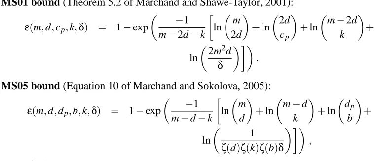
• MS01 bound (Theorem 5.2 of Marchand and Shawe-Taylor, 2001):

ε(m,d,cp,k,δ) = 1−exp

−1

m−2d−k

ln

m

2d

+ln

2d

cp

+ln

m−2d

k

+

ln

2m2d δ

.

• MS05 bound (Equation 10 of Marchand and Sokolova, 2005):

ε(m,d,dp,b,k,δ) = 1−exp

−1

m−d−k

ln

m d

+ln

m−d k

+ln

dp b

+

ln

1

ζ(d)ζ(k)ζ(b)δ

,

whereζ(a)is given by Equation 6.

5.2 Discussion of Results

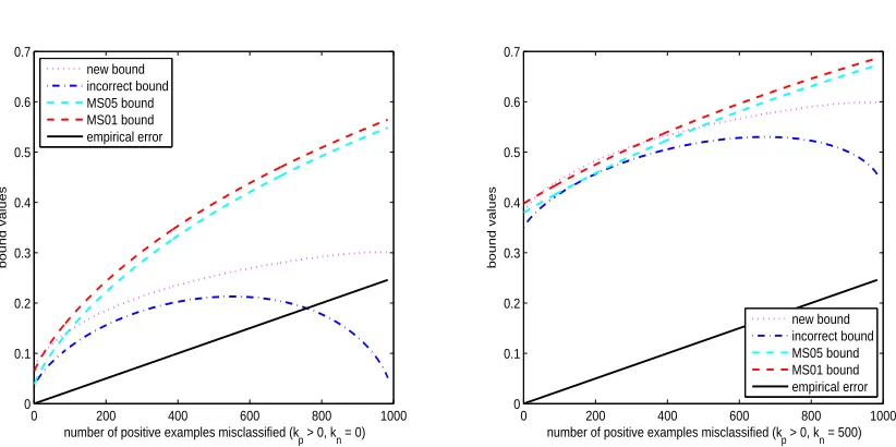
The numerical comparisons of these four bounds (new bound, incorrect bound, MS01 bound and

MS05 bound) are shown in Figure 1 and Figure 2. Each plot contains the number of positive

ex-amples mp, the number of negative examples mn, the number of positive centers cp, the number of negative centers cnand the number of borders b. The number of negative misclassifications knwas fixed for all plots and these values can be found in the x-axis label (either 0 or 500). The number of positive examples was varied and its quantity was set to those values given by the x-axis of the plot. For example, in the left hand side plot of Figure 1, the number of negative misclassifications knwas 0 and the number of positive misclassifications kpvaried from 1 to 2000. The y-axis give the bound values achieved. Finally, the empirical error was also included in each plot—which is simply the number of examples misclassified divided by the number of examples, that is,(kp+kn)/(mp+mn). Figure 1 shows the case where the number of positive and negative examples is approximately the same. We clearly see that the incorrect bound becomes erroneous when the number kpof errors on the positive training examples approaches the total number mpof positive training examples. We also see that the new bound is tighter than the MS01 and MS05 bounds when the kpdiffers greatly from kn. However, the latter bound is slightly tighter than the new bound when kp=kn.

Figure 2 depicts the case where there is an imbalance in the data set (mnmp), implying greater possibility of imbalance in misclassifications. However, the behavior is similar as the one found in Figure 1. Indeed, the MS01 and MS05 loss bounds are slightly smaller than the new bound when

0 500 1000 1500 2000 0

0.1 0.2 0.3 0.4 0.5 0.6 0.7 0.8

number of positive examples misclassified (k_p > 0, k_n = 0)

bound values

new bound incorrect bound MS05 bound MS01 bound empirical error

0 500 1000 1500 2000

0.1 0.2 0.3 0.4 0.5 0.6 0.7 0.8 0.9

number of positive examples misclassified (k_p > 0, k_n = 500)

bound values

new bound incorrect bound MS05 bound MS01 bound empirical error

Figure 1: Bound values for the SCM when mp=2020,mn=1980,cp=5,cn=5,b=10.

0 200 400 600 800 1000

0 0.1 0.2 0.3 0.4 0.5 0.6 0.7

number of positive examples misclassified (k_p > 0, k_n = 0)

bound values

new bound incorrect bound MS05 bound MS01 bound empirical error

0 200 400 600 800 1000

0 0.1 0.2 0.3 0.4 0.5 0.6 0.7

number of positive examples misclassified (k_p > 0, k_n = 500)

bound values

new bound incorrect bound MS05 bound MS01 bound empirical error

6. Conclusion

We have observed that the SCM loss bound proposed by Marchand and Shawe-Taylor (2002) is incorrect and, in fact, becomes erroneous in the limit where the number of errors on the positive training examples approaches the total number of positive training examples. We have then pro-posed a new loss bound, valid for any sample-compression learning algorithm (including the SCM), that depends on the observed fraction of positive examples and on what the classifier achieves on them. This new bound captures the spirit of Marchand and Shawe-Taylor (2002) with very similar tightness in the regimes in which the bound could hold. This is shown in numerical comparisons of the loss bound proposed in this paper with all of the earlier bounds that can be applied to the SCM. As mentioned above, an advantage of the bound is its ability to take into account the observed number of positive examples in the training set in order to arrive at tighter estimates. It also has the advantage of being applicable in cases where the loss function is asymmetrical for type I and type II errors, a situation that is not uncommon in practical applications.

The tightness of the bounds derived for the set covering machine make it tempting to use them to perform model selection as well as to consider integrating them more closely into the workings of the algorithm. Both of these directions are the subject of ongoing research.

Acknowledgments

We would like to thank the anonymous reviewers for their helpful comments. This work was sup-ported by NSERC Discovery grants 262067 and 122405 and, in part, by the IST Programme of the European Community, under the PASCAL Network of Excellence, IST-2002-506778. This publi-cation only reflects the authors’ views.

References

Sally Floyd and Manfred Warmuth. Sample compression, learnability, and the Vapnik-Chervonenkis dimension. Machine Learning, 21(3):269–304, 1995.

John Langford. Tutorial on practical prediction theory for classification. Journal of Machine

Learn-ing Research, 6:273–306, 2005.

Nick Littlestone and Manfred Warmuth. Relating data compression and learnability. Technical report, University of California Santa Cruz, Santa Cruz, CA, 1986.

Mario Marchand and John Shawe-Taylor. Learning with the set covering machine. Proceedings

of the Eighteenth International Conference on Machine Learning (ICML 2001), pages 345–352,

2001.

Mario Marchand and John Shawe-Taylor. The set covering machine. Journal of Machine Learning

Reasearch, 3:723–746, 2002.

Mario Marchand and Marina Sokolova. Learning with decision lists of data-dependent features.