The Pyramid Match Kernel: Efficient Learning with Sets of Features

The Pyramid Match Kernel: Efficient Learning with Sets of Features

Kristen Grauman [email protected]

Department of Computer Sciences University of Texas at Austin Austin, TX 78712, USA

Trevor Darrell [email protected]

Computer Science and Artificial Intelligence Laboratory Massachusetts Institute of Technology

Cambridge, MA 02139, USA

Editor: Pietro Perona

Abstract

In numerous domains it is useful to represent a single example by the set of the local features or parts that comprise it. However, this representation poses a challenge to many conventional machine learning techniques, since sets may vary in cardinality and elements lack a meaningful ordering. Kernel methods can learn complex functions, but a kernel over unordered set inputs must somehow solve for correspondences—generally a computationally expensive task that becomes impractical for large set sizes. We present a new fast kernel function called the pyramid match that measures partial match similarity in time linear in the number of features. The pyramid match maps unordered feature sets to multi-resolution histograms and computes a weighted histogram intersection in order to find implicit correspondences based on the finest resolution histogram cell where a matched pair first appears. We show the pyramid match yields a Mercer kernel, and we prove bounds on its error relative to the optimal partial matching cost. We demonstrate our algorithm on both classification and regression tasks, including object recognition, 3-D human pose inference, and time of publication estimation for documents, and we show that the proposed method is accurate and significantly more efficient than current approaches.

Keywords: kernel, sets of features, histogram intersection, multi-resolution histogram pyramid,

approximate matching, object recognition

1. Introduction

In a variety of domains, it is often natural and meaningful to represent a data object with a collection of its parts or component features. For instance, in computer vision, an image may be described by local features extracted from patches around salient interest points, or a shape may be described by local descriptors defined at edge pixels. Likewise, in natural language processing, documents or topics may be represented by sets or bags of words; in computational biology, a disease may be characterized by sets of gene-expression data from multiple patients. In such cases, one set of feature vectors denotes a single instance of a particular class of interest (an object, shape, document, etc.). The number of features per example varies, and within a single instance the component features may have no inherent ordering.

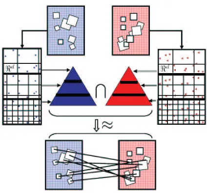
Figure 1: The pyramid match intersects histogram pyramids formed over sets of features, approx-imating the optimal correspondences between the sets’ features. For example, vectors describing the appearance or shape within local image patches can be used to form a fea-ture set for each image; the pyramid match approximates the similarity according to a partial matching in that feature space. (The feature space can be any local description of a data object, images or otherwise; for images the features typically will not be the spatial image coordinates.)

kernels are designed to operate on fixed-length vector inputs, where each dimension corresponds to a particular global attribute for that instance; the commonly used general-purpose kernels defined on

ℜn_{inputs are not applicable in the space of vector sets. Existing kernel-based approaches specially} designed for matching sets of features generally require either solving for explicit correspondences between features (which is computationally costly and prohibits the use of large inputs) or fitting a particular parametric distribution to each set (which makes restrictive assumptions about the data and can also be computationally expensive).

In this work we present the pyramid match kernel—a new kernel function over unordered fea-ture sets that allows them to be used effectively and efficiently in kernel-based learning methods. Each feature set is mapped to a multi-resolution histogram that preserves the individual features’ distinctness at the finest level. The histogram pyramids are then compared using a weighted his-togram intersection computation, which we show defines an implicit correspondence based on the finest resolution histogram cell where a matched pair first appears (see Figure 1).

machine). We also provide theoretical approximation bounds for the pyramid match cost relative to the optimal partial matching cost.

Because it does not penalize the presence of superfluous data points, the proposed kernel is robust to clutter. As we will show, this translates into the ability to handle common issues faced in vision tasks like object recognition or pose estimation: unsegmented images, poor segmentations, varying backgrounds, and occlusions. The kernel also respects the co-occurrence relations inherent in the input sets: rather than matching features in a set individually, ignoring potential dependencies conveyed by features within one set, our similarity measure captures the features’ joint statistics.

Other approaches to this problem have recently been proposed (Wallraven et al. 2003; Lyu 2005; Boughhorbel et al. 2004; Kondor and Jebara 2003; Wolf and Shashua 2003; Moreno et al. 2003; Shashua and Hazan 2005; Cuturi and Vert 2005; Boughorbel et al. 2005; Lafferty and Lebanon 2002), but unfortunately each suffers from some number of the following drawbacks: computational complexities that make large feature set sizes infeasible; limitations to parametric distributions which may not adequately describe the data; kernels that are not positive-definite; limitations to sets of equal size; and failure to account for dependencies within feature sets.

Our method addresses each of these issues, resulting in a kernel appropriate for comparing un-ordered, variable-sized feature sets within any existing kernel-based learning paradigm. We demon-strate our algorithm in a variety of classification and regression tasks: object recognition from sets of image patch features, 3-D human pose inference from sets of local contour features from monoc-ular silhouettes, and documents’ time of publication estimation from bags of local latent semantic features. The results show that the proposed approach achieves an accuracy that is comparable to or better than that of state-of-the-art techniques, while requiring significantly less computation time.

2. Related Work

In this section, we review relevant work on learning with sets of features, using kernels and support vector machines (SVMs) for recognition, and multi-resolution image representations.

Kernel-based learning algorithms, which include SVMs, kernel PCA, and Gaussian Processes, have become well-established tools that are useful in a variety of contexts, including discriminative classification, regression, density estimation, and clustering (Shawe-Taylor and Cristianini, 2004; Vapnik, 1998; Rasmussen and Williams, 2006). However, conventional kernels (such as the Gaus-sian RBF or polynomial) are designed to operate on ℜn vector inputs, where each vector entry corresponds to a particular global attribute for that instance. As a result, initial approaches us-ing SVMs for recognition were forced to rely on global image features—ordered features of equal length measured from the image as a whole, such as color or grayscale histograms or vectors of raw pixel data (Chapelle et al., 1999; Roobaert and Hulle, 1999; Odone et al., 2005). Such global representations are known to be sensitive to real-world imaging conditions, such as occlusions, pose changes, or image noise.

step (e.g., Lowe, 2004; Mikolajczyk and Schmid, 2001); both may be impractical for large training sets, since their classification times increase with the number of training examples. A support vec-tor classifier or regressor, on the other hand, identifies a sparse subset of the training examples (the support vectors) to delineate a decision boundary or approximate a function of interest.

In order to more fully leverage existing kernel-based learning tools for situations where the data cannot be naturally represented by a Euclidean vector space—such as graphs, strings, or trees—researchers have developed specialized similarity measures (Gartner, 2003). In fact, due to the increasing prevalence of data that is best represented by sets of local features, several re-searchers have recently designed kernel functions that can handle unordered sets as input (Lyu 2005; Kondor and Jebara 2003; Wolf and Shashua 2003; Shashua and Hazan 2005; Boughhorbel et al. 2004; Boughorbel et al. 2005; Wallraven et al. 2003; Cuturi and Vert 2005; Moreno et al. 2003; Lafferty and Lebanon 2002). Nonetheless, current approaches are either pro-hibitively computationally expensive, are forced to make assumptions regarding the parametric form of the features, discard information by replacing inputs with prototypical features, ignore important co-occurrence information by considering features independently, are not positive-definite, and (or) are limited to sets of equal size. In addition, none have shown the ability to learn a real-valued function from sets of features; results have only been shown for classification tasks. See Figure 2 for a concise comparison of the approaches.

Approaches which fit a parametric model to feature sets in order to compare their distributions (Kondor and Jebara, 2003; Moreno et al., 2003; Cuturi and Vert, 2005; Lafferty and Lebanon, 2002) can be computationally costly and have limited applicability, since they assume both that features within a set will conform to the chosen distribution, and that sets will be adequately large enough to extract an accurate estimate of the distribution’s parameters. These assumptions are violated regu-larly by real data, which will often exhibit complex variations within a single bag of features (e.g., patches from an image), and will produce wide ranges of cardinalities per instance (e.g., titles of documents have just a few word features). Our method instead takes a non-parametric, “model-free” approach, representing sets of features directly with multi-dimensional, multi-resolution histograms.

Kernel methods that use explicit correspondences between two sets’ features search one set for the best matching feature for each member in the other, and then define set similarity as a func-tion over those component similarity values (Wallraven et al., 2003; Lyu, 2005; Boughhorbel et al., 2004; Boughorbel et al., 2005). These methods have complexities that are quadratic in the number of features, hindering usage for kernel-based learning when feature sets are large. The “intermedi-ate” matching kernel of Boughorbel et al. (2005) has a quadratic run-time if the number of proto-types p=O(m). That is reduced if p is set so that p<m; however, the authors note that higher

values of p yield more accurate results. Furthermore, matching each input feature independently ignores useful information about intra-set dependencies. In contrast, our kernel captures the joint statistics of co-occurring features by matching them concurrently as a set.

Captures Positive- Handles unequal Method Complexity co-occurrences definite Non-parametric cardinalities

Match O(dm2) x x

Exponent match O(dm2) x x x

Greedy match O(dm2) x x x

Principal angles O(dm3) x x

Intermediate O(d pm) x x x

Bhattacharyya’s O(dm3) x x x

KL-divergence O(dm2) x x

Pyramid match O(dm log D) x x x x

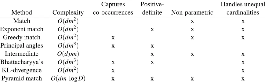
Figure 2: Comparing the properties of kernel approaches to matching unordered sets. “Match” refers to the kernel of Wallraven et al. (2003), “Exponent match” is the kernel of Lyu (2005), “Greedy match” is from Boughhorbel et al. (2004), “Principal angles” is from Wolf and Shashua (2003), “Intermediate” is from Boughorbel et al. (2005), “Bhattacharyya’s” is from Kondor and Jebara (2003), and “KL-divergence” is from Moreno et al. (2003). “Pyramid match” refers to the proposed kernel. Each method’s computational cost is for computing a single kernel value. d is vector dimension, m is maximum set cardinality, p is the number of prototype features used by Boughorbel et al. (2005), and D is the value of the maximal feature range.

Several computer vision researchers have transformed the set of real-valued feature vectors com-ing from one image into a scom-ingle flat histogram that counts the frequency of occurrence of some num-ber of pre-defined (quantized) feature prototypes. In this way the quantized feature space provides a visual vocabulary or bag-of-words vector representation which can be used in conjunction with some vector-based kernels or similarity measures. This type of representation was explored for tex-ture recognition using nearest-neighbors (Leung and Malik, 2001; Hayman et al., 2004), and more recently has been shown for classification of object categories using SVMs, Na¨ıve Bayes classifiers, and a probabilistic Latent Semantic Analysis framework (Csurka et al., 2004; Willamowski et al., 2004; Sivic et al., 2005).

An alternative approach to discriminative classification when dealing with unordered set data is to designate prototypical examples from each class, and then represent examples by a vector giving their distances to each prototype; standard algorithms that handle vectors in a Euclidean space are then applicable. Zhang and Malik (2003) build such a classifier for handwritten digits, and use the shape context distance of Belongie et al. (2002) as the measure of similarity. Shan et al. also explore a representation based on distances to prototypes in order to avoid feature matching when recogniz-ing vehicles (Shan et al., 2005). The issues faced by such a prototype-based method are determinrecogniz-ing which examples should serve as prototypes, choosing how many there should be, and updating the prototypes properly when new types of data are encountered. The method of Holub et al. (2005a) uses a hybrid generative-discriminative approach for object recognition, combining the Fisher ker-nel (Jaakkola and Haussler, 1999) and a probabilistic constellation model.

Our feature representation is based on a multi-resolution histogram, or pyramid, which is com-puted by binning data points into discrete regions of increasingly larger size. Single-level histograms have been used in various visual recognition systems, one of the first being that of Swain and Ballard (1991), where the intersection of global color histograms was used to compare images. Pyra-mids have been shown to be a useful representation in a wide variety of image processing tasks, from image coding (Burt and Adelson, 1983), to optical flow (Anandan, 1987), to texture modeling (Malik and Perona, 1990). See work by Hadjidemetriou et al. (2004) for a summary.

In the method of Indyk and Thaper (2003), multi-resolution histograms are compared with L1 distance to approximate a least-cost matching of equal-mass global color histograms for nearest neighbor image retrievals. This work inspired our use of a similar representation for point sets and to consider counting matches within histograms. However, in contrast Indyk and Thaper’s approach, our method builds a discriminative classifier or regressor over sets of local features, and it allows inputs to have unequal cardinalities. Most importantly, it enables partial matchings, which is important in practice for handling clutter and unsegmented images. In addition, we show that our approximate matching forms a valid Mercer kernel and explore its use for kernel-based learning for various applications.

In this work we develop a new kernel function that efficiently handles inputs that are unordered sets of varying sizes. We show how the pyramid match kernel may be used in conjunction with existing kernel-based learning algorithms to successfully learn decision boundaries or real-valued functions from the multi-set representation. Ours is the first work to show the histogram pyramid’s connection to the optimal partial matching when used with a hierarchical weighted histogram inter-section similarity measure.1

3. Approach

The main contribution of this work is a new kernel function based on implicit correspondences that enables discriminative classification and regression for unordered, variable-sized sets of vectors. The kernel is provably positive-definite. The main advantages of our algorithm are its efficiency, its use of the joint statistics of co-occurring features, and its resistance to clutter or “superfluous”

data points. The basic idea of our method is to map sets of features to multi-resolution histograms, and then compare the histograms with a weighted histogram intersection measure in order to ap-proximate the similarity of the best partial matching between the feature sets. We call the proposed matching kernel the pyramid match kernel because input sets are converted to multi-resolution his-tograms.

3.1 Preliminaries

We consider a feature space F of d-dimensional vectors. The point sets (or multi-sets, since dupli-cations of features may occur within a single set) we match will come from the input space S, which contains sets of feature vectors drawn from F:

S=nX_|X=_{x1, . . . ,xm}

o

,

where each feature is a d-dimensional vector, xi ∈F ⊆ℜd, and m=|X|. Note that the point dimension d is fixed for all features in F, but the value of m may vary across instances in S. The values of elements in vectors in F have a maximal range D, and the minimum inter-vector distance between unique points is 1, which may be enforced by scaling the data to some precision and truncating to integer values.

In this work we want to efficiently approximate the optimal partial matching. A partial matching between two point sets is an assignment that maps all points in the smaller set to some subset of the points in the larger (or equally-sized) set. Given point sets X and Y, where m=_|X_|, n=_|Y_|, and

m≤n, a partial matching

M

(X,Y;π) =_{(x1,yπ1), . . . ,(xm,yπm)}

pairs each point in X to some unique point in Y according to the permutation of indices specified byπ= [π1, . . . ,πm], 1≤πi ≤n, whereπi specifies which point yπi ∈Y is matched to xi∈X, for

1_≤i_≤m. The cost of a partial matching is the sum of the distances between matched points:

C

(

M

(X,Y;π)) =

∑

xi∈X

||xi−yπi||1.

The optimal partial matching

M

(X,Y;π∗)uses the assignmentπ∗that minimizes this cost:

π∗_=argmin

π

C

(

M

(X,Y;π)). (1)

In order to form a kernel function based on correspondences, we are interested in evaluating partial matching similarity, where similarity is measured in terms of inverse distance or cost. The similarity

S

(

M

(X,Y;π))of a partial matching is the sum of the inverse distances between matched points:

S

(

M

(X,Y;π)) =

∑

xi∈X

1 ||xi−yπi||1+1

,

3.2 The Pyramid Match Algorithm

The pyramid match approximation uses a multi-dimensional, multi-resolution histogram pyramid to partition the feature space into increasingly larger regions. At the finest resolution level in the pyramid, the partitions (bins) are very small; at successive levels they continue to grow in size until the point where a single partition encompasses the entire feature space. At some level along this gradation in bin sizes, any two points from any two point sets will begin to share a bin, and when they do, they are considered matched. The pyramid allows us to extract a matching score without computing distances between any of the points in the input sets—when points sharing a bin are counted as matched, the size of that bin indicates the farthest distance any two points in it could be from one another.

Each feature set is mapped to a multi-resolution histogram that preserves the individual features’ distinctness at the finest level. The histogram pyramids are then compared using a weighted his-togram intersection computation, which we show defines an implicit partial correspondence based on the finest resolution histogram cell where a matched pair first appears. The computation time of both the pyramids themselves as well as the weighted intersection is linear in the number of features.

The feature extraction functionΨfor an input set X is defined as:

Ψ(X) = [H0(X), . . . ,HL−1(X)], (2)

where X_∈S, L=_dlog₂D_e+1, Hi(X) is a histogram vector formed over points in X using d-dimensional bins of side length 2i, and Hi(X)has a dimension ri= ₂Di

d

. In other words,Ψ(X)is a histogram pyramid, where each subsequent component histogram has bins that double in size (in all d dimensions) compared to the previous one. The bins in the finest-level histogram H0are small enough that each unique d-dimensional data point from features in F falls into its own bin, and then the bin size increases until all points in F fall into a single bin at level L−1.2

The pyramid match

P

_∆ measures similarity (or dissimilarity) between point sets based on im-plicit correspondences found within this multi-resolution histogram space. The similarity between two input sets Y and Z is defined as the weighted sum of the number of feature matchings found at each level of the pyramid formed byΨ:

P

∆(Ψ(Y),Ψ(Z)) = L−1

∑

i=0

wiNi, (3)

where Ni signifies the number of newly matched pairs at level i, and wi is a weight for matches formed at level i (and will be defined below). A new match is defined as a pair of features that were not in correspondence at any finer resolution level.

The matching approximation implicitly finds correspondences between point sets, if we con-sider two points matched once they fall into the same histogram bin, starting at the finest resolution level where each unique point is guaranteed to be in its own bin. The correspondences are implicit in that matches are counted and weighted according to their strength, but the specific pairwise links be-tween points need not be individually enumerated. The matching is a hierarchical process: vectors not found to correspond at a fine resolution have the opportunity to be matched at coarser resolu-tions. For example, in Figure 3, there are two points matched at the finest scale, two new matches at

y z

y z

y z

(a) Point sets

H

0(y) H0(z)

H

1(y) H1(z)

H

2(y) H2(z)

(b) Histogram pyramids

min(H

0(y), H0(z))

I

0=2

min(H

1(y), H1(z))

I

1=4

min(H

2(y), H2(z))

I

2=5

(c) Intersections

N

0=2−0=2

w₀=1

N₁=4−2=2

w₁=1/2

N₂=5−4=1

w

2=1/4

(d) New

matches

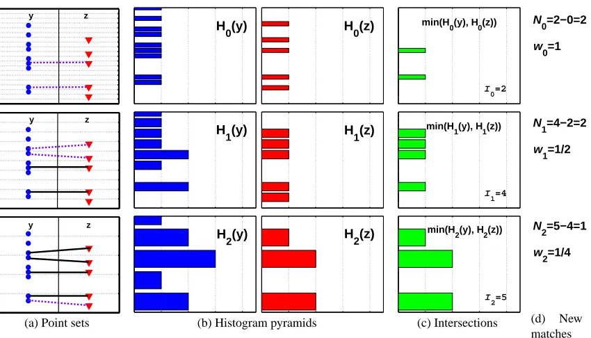
Figure 3: The pyramid match (

P

_∆) determines a partial correspondence by matching points once they fall into the same histogram bin. In this example, two 1-D feature sets are used to form two histogram pyramids. Each row corresponds to a pyramid level. In (a), the set Y is on the left side, and the set Z is on the right. (Points are distributed along the vertical axis, and these same points are repeated at each level.) Light dotted lines are bin boundaries, bold dashed lines indicate a new pair matched at this level, and bold solid lines indicate a match already formed at a finer resolution level. In (b) multi-resolution histograms are shown, with bin counts along the horizontal axis. In (c) the intersection pyramids between the histograms in (b) are shown.

P

∆ uses these intersection counts to measure how many new matches occurred at each level. Here,

I

i =

I

(Hi(Y),Hi(Z)) = 2,4,5 across levels, and therefore the number of new matches found at each level are

Ni=2,2,1. (

I

−1=0 by definition.) The sum over Ni, weighted by wi=1,1₂,1₄, gives the pyramid match similarity.

the medium scale, and one at the coarsest scale.

P

_∆’s output value reflects the overall similarity of the matching: each newly matched pair at level i contributes a value withat is proportional to how similar two points matching at that level must be, as determined by the bin size.

To calculate Ni, the pyramid match makes use of a histogram intersection function

I

, which measures the “overlap” between two histograms’ bin counts:

I

(A,B) = r

∑

j=1 min

A(j),B(j)

,

Histogram intersection effectively counts the number of points in two sets that match at a given quantization level, that is, fall into the same bin. To calculate the number of newly matched pairs

Niinduced at level i, it is sufficient to compute the difference between successive histogram levels’ intersections:

Ni=

I

(Hi(Y),Hi(Z))−

I

(Hi₋1(Y),Hi₋1(Z)), (4)

where Hirefers to the ithcomponent histogram generated byΨin Eqn. 2. Note that the measure is not searching explicitly for similar points—it never computes distances between the vectors in each set. Instead, it simply uses the change in intersection values at each histogram level to count the matches as they occur. In addition, due to the subtraction in Eqn. 4, the output score will reflect an underlying matching that is one-to-one.

The sum in Eqn. 3 starts with index i=0 because by the definition of F, the same points that could match at level 0 can match at (a hypothetical) level ₋1. Therefore we can start col-lecting new match counts at level 0, and define level₋1 to be a base case with no intersections:

I

(H₋1(Y),H−1(Z)) =0. All matches formed at level 0 are new.

The number of new matches found at each level in the pyramid is weighted according to the size of that histogram’s bins: to measure similarity, matches made within larger bins are weighted less than those found in smaller bins. Specifically, we make a geometric bound of the distance between any two points sharing a particular bin; in terms of L1 cost, two points in the same bin can only be as far from one another as the sum of the lengths of the bin’s sides. At level i in a pyramid, this length is equal to d2i. Thus, the number of new matches induced at level i is weighted by

wi=_d21i to reflect the (worst-case) similarity of points matched at that level. Intuitively, this means

that similarity between vectors (features in Y and Z) at a finer resolution—where features are more distinct—is rewarded more heavily than similarity between vectors at a coarser level.3 Moreover, as we show in Section 6, this particular setting of the weights enables us to prove theoretical error bounds for the pyramid match cost.

From Eqns. 3 and 4, we define the (un-normalized) pyramid match:

˜

P

∆(Ψ(Y),Ψ(Z)) = L−1

∑

i=0

wi

I

(Hi(Y),Hi(Z))−

I

(Hi−1(Y),Hi−1(Z))

, (5)

where Y,Z_∈S, and Hi(Y)and Hi(Z) refer to the ith histogram inΨ(Y) andΨ(Z), respectively. We normalize this value by the product of each input’s self-similarity to avoid favoring larger input sets, arriving at the final kernel value

P

_∆(P,Q) =_√1

C

P

˜∆(P,Q), where C=

P

˜∆(P,P)

P

˜∆(Q,Q). In order to alleviate quantization effects that may arise due to the discrete histogram bins, we combine the kernel values resulting from multiple (T ) pyramid matches formed under different multi-resolution histograms with randomly shifted bins. Each dimension of each of the T pyramids is shifted by an amount chosen uniformly at random from[0,D]. This yields T feature mappings

Ψ1, . . . ,ΨT that are applied as in Eqn. 2 to map an input set X to T multi-resolution histograms:

[Ψ1(X), . . . ,ΨT(X)]. For inputs Y and Z, the combined kernel value is then∑Tj=1

P

∆(Ψj(Y),Ψj(Z)). To further refine a pyramid match, multiple pyramids with unique initial (finest level) bin sizes may be used. The set of unique bin sizes produced throughout a pyramid determines the range

3. This is if the pyramid match is a kernel measuring similarity; an inverse weighting scheme is applied if the pyramid match is used to measure cost. To use the matching as a cost function, weights are set as the distance estimates

(wi=d2i); to use as a similarity measure, weights are set as (some function of) the inverse of the distance estimates

of distances at which features will be considered for possible matchings. With bin sizes doubling in size at every level of a pyramid, this means that the range of distances considered will rapidly increase until the full diameter of the feature space is covered. However, by incorporating multiple pyramids with unique initial bin sizes, we can boost that range of distances to include more diverse gradations. This is accomplished by setting the side length for each histogram Hi(X)to f 2i, where

f is the side length at the finest resolution (in the above definition, f =1). For example, say D=32,

so L=6. Then the set of distances considered with f =1 are_{1,2,4,8,16,32_}; adding a second pyramid with f =3 increases this set to also consider the distances_{3,6,12,24_}. The outputs from pyramids with multiple starting side lengths are combined in the same way that the outputs from pyramids with multiple translations are combined.

In fact, the rationale for considering multiple random shifts of the pyramid grids is not only to satisfy the intuitive need to reduce quantization effects caused by bin placements; it also allows us to theoretically measure how probable it is (in the expectation) that any two points will be separated by a bin boundary, as we describe below in Section 6.

3.3 Partial Match Correspondences

The pyramid match allows input sets to have unequal cardinalities, and therefore it enables partial matchings, where the points of the smaller set are mapped to some subset of the points in the larger set. Dissimilarity is only judged on the most similar part of the empirical distributions, and superfluous data points from the larger set are entirely ignored; the result is a robust similarity measure that accommodates inputs expected to contain extraneous vector entries. This is a common situation when recognizing objects in images, due for instance to background variations, clutter, or changes in object pose that cause different subsets of features to be visible. As a kernel, the proposed matching measure is equipped to handle unsegmented or poorly segmented examples, as we will demonstrate in Section 9.

Since the pyramid match defines correspondences across entire sets simultaneously, it inherently accounts for the distribution of features occurring in one set. In contrast, previous approaches have used each feature in a set to independently index into the second set; this ignores possibly useful information that is inherent in the co-occurrence of a set of distinctive features, and it fails to distinguish between instances where an object has varying numbers of similar features since multiple features may be matched to a single feature in the other set (Wallraven et al., 2003; Lyu, 2005; Boughorbel et al., 2005; Lowe, 2004; Mikolajczyk and Schmid, 2001; Tuytelaars and Gool, 1999; Shaffalitzky and Zisserman, 2002).

4. Efficiency

A key aspect of this method is that we obtain a measure of matching quality between two point sets without computing pairwise distances between their features—an O(m2)savings over sub-optimal greedy matchings. Instead, we exploit the fact that the points’ placement in the pyramid reflects their distance from one another in the feature space.

The time required to compute the L-level histogram pyramidΨ(X)for an input set with m=_|X_|

d-dimensional features is O(dzL), where z=max(m,k)and k is the maximum histogram index value

in a single dimension. For a histogram at level i, k_≤ D₂i, so at any level, k≤D. (Typically m>k.)

sorted by the bin indices and the bin counts for all entries with the same index are summed to form one entry. This sorting requires only O(dm+dk)time using the radix-sort algorithm with counting sort, a linear time sorting algorithm that is applicable to the integer bin indices Cormen et al. (1990). The histogram pyramid that results is high-dimensional, but very sparse, with only O(mL)nonzero entries that need to be stored.

The computational complexity of

P

_∆ is O(dmL), since computing the intersection values for histograms that have been sorted by bin index requires time linear in the number of nonzero entries (not the number of actual bins). With sorted bin index lists, we obtain the intersection value by running one pointer down each of the two lists; one pointer may not advance until the other is incremented down to an index at least as high as the other, or else the end of its list. Then, whenever the two lists share a nonzero index, the intersection count is incremented by the minimum bin count between the two. If one list has a nonzero count for some bin index but the other has no entry for that index, the minimum count is 0, so no update is needed. In the applications we explore in our experiments, typical values of the variables affecting complexity are as follows: 5_≤d _≤12, 300_≤m_≤3000, and D_≈250, which yields L=9.

Generating multiple pyramid matches with randomly shifted grids scales the complexity by T , the constant number of shifts. (Typically we will use 1≤T ≤3.) All together, the complexity of computing both the pyramids and kernel or cost values is O(T dmL). In contrast, the optimal matching requires O(dm3)time, which severely limits the practicality of large input sizes. Refer to Figure 2 for complexity comparisons with existing set kernels.

5. Satisfying Mercer’s Condition

Kernel-based learning algorithms are founded on the idea of embedding data into a Euclidean space, and then seeking linear relations among the embedded data (Shawe-Taylor and Cristianini, 2004; Vapnik, 1998). For example, a support vector machine (SVM) finds the optimal separating hyper-plane between two classes in an embedded space (also referred to as the feature space). A kernel function K : X_×X _→ ℜ serves to map pairs of data objects in an input space X to their inner product in the embedding space E, thereby evaluating the similarities between all data objects and determining their relative positions. Linear relations are sought in the embedded space, but the learned function may still be non-linear in the input space, depending on the choice of a feature mapping functionΦ: X_→E.

Only positive semi-definite kernels guarantee an optimal solution to kernel-based algorithms based on convex optimization, which includes SVMs. According to Mercer’s theorem, a kernel K is positive semi-definite if and only if there exists a mappingΦsuch that

K(xi,xj) =hΦ(xi),Φ(xj)i, ∀xi,xj∈X,

where_h·,_·idenotes a scalar dot product. This insures that the kernel corresponds to an inner product in some feature space, where kernel methods can search for linear relationships (Shawe-Taylor and Cristianini, 2004).

Proposition 1

Proof:

Histogram intersection on single resolution histograms over multi-dimensional data was shown to be a positive-definite function by Odone et al. (2005). That is, the intersection

I

(H(Y),H(Z))is a Mercer kernel. The proof shows that there is an explicit feature mapping after which the intersection is an inner product. Specifically, the mapping

V

encodes an r-bin histogram H as a p-dimensional binary vector, p=m_×r, where m is the total number of points in the histogram:

V

(H) =



 

H(1)

z }| {

1, . . . ,1,

m₋H(1)

z }| {

0, . . . ,0

| {z }

first bin

, . . . ,

H(r)

z }| {

1, . . . ,1,

m₋H(r)

z }| {

0, . . . ,0

| {z }

last bin





.

The inner product between the binary strings output from

V

is equivalent to the original histograms’ intersection value (Odone et al., 2005). If m varies across examples, the above holds by setting

p=M_×r, where M is the maximum size of any input. Note that this binary encoding only serves

to prove positive-definiteness and is never computed explicitly.

Using this proof and the closure properties of valid kernel functions, we can show that the pyramid match is a Mercer kernel. The definition given in Eqn. 5 is algebraically equivalent to

˜

P

∆(Ψ(Y),Ψ(Z)) =wL₋1

I

(HL₋1(Y),HL₋1(Z)) + L₋2

∑

i=0

(wi−wi+1)

I

(Hi(Y),Hi(Z)),

since

I

(H₋1(Y),H−1(Z)) =0 by definition. Given that Mercer kernels are closed under both addi-tion and scaling by a positive constant (Shawe-Taylor and Cristianini, 2004), the above form shows that the pyramid match kernel is positive semi-definite for any weighting scheme where wi≥wi+1. In other words, if we can insure that the weights decrease for coarser pyramid levels, then the pyra-mid match will sum over positively weighted definite kernels, yielding another positive-definite kernel. Using the weights wi= _d21i, we do maintain this property. The sum combining the

outputs from multiple pyramid matches under different random bin translations likewise remains Mercer. Therefore, the pyramid match is valid for use as a kernel in any existing learning methods that require Mercer kernels.

6. Approximation Error Bounds

In this section we show theoretical approximation bounds on the cost measured by the pyramid match relative to the cost measured by the optimal partial matching defined in Section 3.1. Re-call the cost (as opposed to similarity) is measured by setting wi=d2i in Eqn. 5. In earlier work, Indyk and Thaper (2003) provided bounds for a multi-resolution histogram embedding’s approxi-mation of the optimal bijective matching between inputs with equal cardinality. Some of the main ideas of the proofs below are similar, but they have been adapted and extended to show the expected error bounds for partial matchings, where input sets can have variable numbers of features, and some features do not affect the matching cost.

Proposition 2

For any two point sets X,Y where|X| ≤ |Y|, we have

Proof:

Consider a matching induced by pairing points within the same cells of each histogram Hi. The cost induced by matching two points within a bin having d sides that are each of length 2iis at most d2i under the L1ground distance.

There are no pairings induced by the histograms at level ₋1, so

I

(H₋1(X),H−1(Y)) =0. At level 0 there are

I

(H0(X),H0(Y)) pairs of points that can be matched together within the same bins of H0, which induces a cost no more than d

I

(H0(X),H0(Y)). Then

I

(H1(X),H1(Y))₋

I

(H0(X),H0(Y))new pairs of points are matched at level 1, which induces a cost no more than 2d[

I

(H1(X),H1(Y))₋

I

(H0(X),H0(Y))], and so on.

In general, histogram Hiinduces cost d2i[

I

(Hi(X),Hi(Y))−

I

(Hi−1(X),Hi−1(Y))]. Summing the costs induced by all levels, we have:

C

(

M

(X,Y;π∗)) _≤

L−1

∑

i=0

d2i

I

(Hi(X),Hi(Y))−

I

(Hi−1(X),Hi−1(Y))

≤

P

∆(X,Y),

where wi=d2iin Eqn. 5.

Proposition 3

There is a constant C such that for any two point sets X and Y, where_|X_{| ≤ |}Y_|, if the histogram bin boundaries are shifted randomly in the same way when computingΨ(X)andΨ(Y), then the expected value of the pyramid match cost is bounded:

E[

P

_∆(X,Y)]_≤C_·d log D+d

C

(

M

(X,Y;π∗)).

Proof:

To write the pyramid match in terms of counts of unmatched points in the implicit partial matching, we define the directed distance between two histograms formed from point sets X and Y:

D

(H(X),H(Y)) =

r

∑

j=1

D

j

H(X)(j),H(Y)(j) , where

D

j(a,b) =

a₋b, if a>b

0, otherwise.

The directed distance

D

(Hi(X),Hi(Y))counts the number of unmatched points at resolution level

i. Note that

D

(H₋1(X),H₋1(Y)) =_|X_|and

D

(HL₋1(X),HL₋1(Y)) =0 by definition. The directed

distance value decreases with i, as bins are increasing in size and more implicit matches are made. The change in the directed distance across levels is the decrease in the count of unmatched points from one level to the next, and therefore also serves to count the number of new matches formed at level i:

In terms of the directed distance, the pyramid match cost is

P

∆(X,Y) =

L−1

∑

i=0

d2i

D

(Hi−1(X),Hi−1(Y))−

D

(Hi(X),Hi(Y))

= d

D

(H₋1(X),H−1(Y)) + L−2

∑

i=0

d2i

D

(Hi(X),Hi(Y))

= d_|X_|+

L−2

∑

i=0

d2i

D

(Hi(X),Hi(Y)).

The expected value of the pyramid match cost is then

E[

P

_∆(X,Y)] =d_|X_|+ L−2

∑

i=0

d2iE[

D

(Hi(X),Hi(Y))]. (6)

The optimal partial matching

M

(X,Y;π∗) =(x1,yπ∗₁), . . . ,(xm,yπ∗

m) implies a graph whose

nodes are those points in the input sets X and Y that participate in the matching (i.e., all points in X and a subset from Y), and whose edges connect the matched pairs(xi,yπi), for 1≤i≤ |X|. Let njbe the number of edges in this graph that have lengths in the range[d2j−1,d2j). A bound on the optimal partial matching may then be expressed as:

∑

j

njd2j−1 ≤

C

(

M

(X,Y;π∗)), or

∑

j

njd2j ≤ 2

C

(

M

(X,Y;π∗)), (7)

since for every j, all njedges must be of length at least d2j−1.

The directed distance

D

counts at a given resolution how many points from set X are unmatched. Any edge in the optimal matching graph that is left “uncut” by the bin boundaries in histogram Hi contributes nothing to

D

(Hi(X),Hi(Y)). Any edge that is “cut” by the histogram contributes at most 1 to

D

(Hi(X),Hi(Y)). Therefore, the expected value of the directed distance at a given resolution is bounded by:

E[

D

(Hi(X),Hi(Y))]≤

∑

j

E[Ti j], (8)

where Ti j is the number of edges in the optimal matching having lengths in the range[d2j−1,d2j) that are cut by Hi.

The probability Pr(cut(x,y); i) that an edge for (x,y) in the optimal matching is cut by the histogram grid Hi is bounded by ||x−₂yi||1. This can be seen by considering the probability of a bin

boundary cutting an edge in any one of the d dimensions, taking into account that the bin boundaries are shifted independently in each dimension. An edge with length_||x₋y_||1>d2i is certainly cut by the histogram grid at Hi. An edge with length||x−y||1≤d2i may be cut in any dimension. In this case, the probability of a cut in dimension k for points x= [x1, . . . ,xd],y= [y1, . . . ,yd]is |xk−₂iyk|,

for 1_≤k_≤d. The probability of a cut from Hioccurring in some dimension is then bounded by the sum of these probabilities:

Pr(cut(x,y); i) _≤ d

∑

k=1

|xk−yk| 2i

This provides an upper bound on the expected number of edges in the optimal matching that are cut at level i:

E[Ti j]≤nj

d2j

2i ,

since by definition d2j is the maximum distance between any pair of matched points counted by nj. Now with Eqns. 7 and 8 we have a bound for the expected directed distance at a certain resolu-tion level:

E[

D

(Hi(X),Hi(Y))]≤ 1 2i

∑

j

njd2j≤

1

2i 2

C

(

M

(X,Y;π∗)).

Relating this to the expected value of the pyramid match cost in Eqn. 6, we have

E[

P

∆(X,Y)] _≤ d_|X_|+

L₋2

∑

i=0

d2i

1

2i 2

C

(

M

(X,Y;π∗))

≤ d|X|+2d(L−1)

C

(

M

(X,Y;π∗))

≤ d_|X_|+2d log D

C

(

M

(X,Y;π∗)) (9)

since L=_dlog₂D_e+1.

As described in Section 3.1, points in sets X and Y are comprised of integer entries, insuring that the minimum inter-feature distance between unique points is 1. We also know that for the sake of measuring matching cost, X and Y are disjoint sets: X_∩Y= /0; if there are any identical points in the two sets, we can consider them as discarded (in pairs) to produce strictly disjoint sets, since identical points contribute nothing to the matching cost. Since X,Y_⊆[D]d_{and X∩Y=/0, we have}

|X_{| ≤}

C

(

M

(X,Y;π∗)). That is, each edge in the optimal matching must have a length of at least 1, making the number of points in the smaller set a lower bound on the cost of the optimal matching for any two sets. With this bound and Eqn. 9, we have the following bound on the expected pyramid match cost error

E[

P

_∆(X,Y)] _≤ d

C

(

M

(X,Y;π∗)) +2d log D

C

(

M

(X,Y;π∗))

≤ 2d log D+d

C

(

M

(X,Y;π∗))

≤ C_·d log D+d

C

(

M

(X,Y;π∗)).

7. Classification and Regression with the Pyramid Match

We train support vector machines and support vector regressors (SVRs) to perform classification and regression with the pyramid match kernel. An SVM or SVR is trained by specifying the matrix of kernel values between all pairs of training examples. The kernel’s similarity values determine the examples’ relative positions in an embedded space, and quadratic programming is used to find the optimal separating hyperplane or function between the two classes in this space. Because the pyramid match kernel is positive-definite we are guaranteed to find a unique optimal solution.

intersections will receive lower weights due to the _d21i weighting scheme, which by construction

accurately reflects the maximal distance between points falling into the same bin at level i. On the other hand, an input set compared against itself will result in large histogram intersection values at each level—specifically intersection values equal to the number of points in the set, which after normalization generates a diagonal entry of one.

The danger of having a kernel matrix diagonal that is significantly larger than the off-diagonal entries is that the examples appear nearly orthogonal in the feature space, in some cases causing an SVM or SVR to essentially “memorize” the data and impairing its sparsity and generalization ability (Shawe-Taylor and Cristianini, 2004). Nonetheless, we are able to work around this issue by modifying the initial kernel matrix in such a way that reduces its dynamic range, while preserving its positive-definiteness. We use the functional calculus transformation suggested in Weston et al. (2002): a subpolynomial kernel is applied to the original kernel values, followed by an empirical kernel mapping that embeds the distance measure into a feature space. Thus, when necessary to reduce diagonal dominance, first kernel values Ki j generated by

P

∆ are updated to Ki j ←Ki jp, 0<p<1. Then the kernel matrix K is replaced with KKT to obtain the empirical feature map

Φe(y) = [K(y,x1), . . . ,K(y,xN)]Tfor N training examples. As in Weston et al. (2002), the parameter

p is chosen with cross-validation. This post-processing of the kernel matrix is not always necessary;

both the dimension of the points as well as the specific structure of a given data set will determine how large the initial kernel matrix diagonal is.

8. Empirical Quality of Approximate Partial Matchings

The approximation bounds we can show are actually significantly weaker than what we observe in practice. In this section, we empirically evaluate the approximation quality of the pyramid match, and make a direct comparison between our partial matching approximation and the L1embedding of Indyk and Thaper (2003).

We conducted experiments to evaluate how close the correspondences implicitly measured by the pyramid match are to the true optimal correspondences—the matching that results in the minimal summed cost between corresponding points. In order to work with realistic data but still have control over the sizes of the sets and the amount of clutter features, we established synthetic “category” models. Each model is comprised of some fixed number m0of parts, and each part has a Gaussian model that generates its d-dimensional appearance vector (in the spirit of the “constellation model” used by Fergus et al., 2003, and others). Given these category models, we can then add clutter features, adjust noise parameters, and so on, simulating in a controlled manner the variations that occur with the sets of image patches extracted from an actual object. The appearance of the clutter features is determined by selecting a random vector from a uniform distribution on the same range of values as the model features.

those produced by an L1 approximation (Indyk and Thaper, 2003). For both of the data sets, we computed the pairwise set-to-set distances using each of these three measures.

If an approximate measure is approximating the optimal matching well, we should find the ranking induced by that approximation to be highly correlated with the ranking produced by the optimal matching for the same data. In other words, the point sets should be sorted similarly by either method. We can display results in two ways to evaluate if this is true: 1) by plotting the actual costs computed by the optimal and approximate method, and 2) by plotting the rankings induced by the optimal and approximate method. Spearman’s rank correlation coefficient R provides a good quantitative measure to evaluate the ranking consistency:

R=1₋6∑

N

i=1(i−ˆr(i))2

N(N2₋₁₎ ,

where i is the rank value in the true order and ˆr(i)is the corresponding rank assigned in the approx-imate ordering, for each of the N corresponding ordinal values assigned by the two measures.

Figure 4 displays both types of plots for the two data sets: the top row (a) displays plots corre-sponding to the data set with equally-sized sets, that is, for the bijective matching problem, while the bottom row (b) displays plots corresponding to the data set with variable-sized sets, that is, for the partial matching problem.

The two plots in the lefthand column show the normalized output costs from 10,000 pairwise set-to-set comparisons computed by the optimal matching (black), the pyramid match with the num-ber of random shifts T=3 (red circles), and the L1approximation, also with T=3 (green x’s). Note that in these figures we plot cost (so the pyramid match weights are set to wi =d2i), and for dis-play purposes the costs have been normalized by the maximum cost produced for each measure to produce values between [0,1]. The cost values are sorted according to the optimal measure’s magnitudes for visualization purposes. The raw values produced by the approximate measures will always overestimate the cost; normalizing by the maximum cost value simply allows us to view them against the optimal measure on the same scale.

The two plots in the righthand column display the rankings for each approximation plotted against the optimal rankings. The black diagonals in these plots denote the optimal performance, where the approximate rankings would be identical to the optimal ones. The R values displayed in the legends refer to the Spearman rank correlation scores for each approximation in that experiment; higher Spearman correlations have points clustered more tightly along this diagonal.

Both approximations compute equivalent costs and rankings for the bijective matching case, as indicated by Figure 4 (a). This is an expected outcome, since the L1distance over histograms is directly related to histogram intersection if those histograms have equal masses (Swain and Ballard, 1991), as they do for the bijective matching test:

I

(H(Y),H(Z)) =m₋1

2||H(Y)−H(Z)||L1, if m=|Y|=|Z|.

0 2000 4000 6000 8000 10000 0 0.1 0.2 0.3 0.4 0.5 0.6 0.7 0.8 0.9 1

Pairwise example matches (sorted according to optimal)

Cost (normalized)

Bijective matching: cost accuracy

Pyramid match L1

Optimal

0 2000 4000 6000 8000 10000 0 1000 2000 3000 4000 5000 6000 7000 8000 9000 10000 Approximation ranks Optimal ranks

Bijective matching: ranking quality

Pyramid match (R=0.89) L1 (R=0.89) Optimal

(a) Bijective matching

0 2000 4000 6000 8000 10000

0 0.1 0.2 0.3 0.4 0.5 0.6 0.7 0.8 0.9 1

Pairwise example matches (sorted according to optimal)

Cost (normalized)

Partial matching: cost accuracy

Pyramid match L1

Optimal

0 2000 4000 6000 8000 10000 0 1000 2000 3000 4000 5000 6000 7000 8000 9000 10000 Approximation ranks Optimal ranks

Partial matching: ranking quality

Pyramid match (R=0.95) L1 (R=−0.69) Optimal

(b) Partial matching

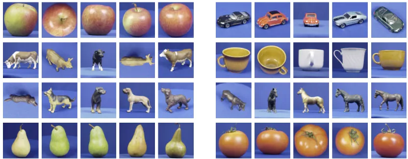
Figure 5: Example images from the ETH-80 objects database. Five images from each of the eight object classes (apple, cow, dog, pear, car, cup, horse, and tomato) are shown here.

in the left plot of part (a) due to distance clusters caused by drawing point sets from two distinct category models.

However, for the partial matching case (Figure 4 (b)), the L1approximation fails because it can handle only sets with equal cardinalities and requires all points to match to something. In contrast, the pyramid match can also approximate the partial matching for the unequal cardinality case: its matchings continue to follow the optimal matching’s trend since it does not penalize outliers, as evidenced by the clustered points along the diagonal in the bottom right ranking quality plot. We have performed this same experiment using data generated from a uniform random point model, and the outcome was similar.

9. Discriminative Classification using Sets of Local Features

In this section we report on object recognition experiments using SVMs and provide baseline com-parisons to other methods. We use the SVM implementation provided in the LIBSVM library (Chang and Lin, 2001) and train one-versus-all classifiers in order to perform multi-class classifica-tion.

Local affine- or scale-invariant feature descriptors extracted from a sparse set of interest points in an image have been shown to be an effective, compact representation (e.g., Lowe 2004; Mikolajczyk and Schmid 2001). This is a good context in which to test the pyramid match ker-nel, since such local features have no inherent ordering, and it is expected that the number of fea-tures will vary across examples. Given two sets of local image feafea-tures, the pyramid match kernel (PMK) value reflects how well the image parts match under a one-to-one correspondence. Since the matching is partial, not all parts must have a match for the similarity to be strong.

9.1 ETH-80 Data Set

A performance evaluation given by Eichhorn and Chapelle (2004) compares the set kernels de-veloped by Kondor and Jebara (2003), Wolf and Shashua (2003), and Wallraven et al. (2003) in the context of an object categorization task using images from the publicly available ETH-80 database.4 The experiment uses eight object classes, with 10 unique objects and five widely separated views of each, for a total of 400 images (see Figure 5). A Harris detector is used to find interest points in each image, and various local descriptors (SIFT features, Lowe 2004; JETs, Schmid and Mohr 1997; and raw image patches) are used to compose the feature sets. A one-versus-all SVM classifier is trained for each kernel type, and performance is measured via cross-validation, where all five views of an object are held out at once. Since no instances of a test object are ever present in the training set, this is a categorization task (as opposed to recognition of the same specific object).

The experiments show the polynomial-time “match kernel” (Wallraven et al., 2003) and Bhat-tacharyya kernel (Kondor and Jebara, 2003) performing best, with a classification rate of 74% using on average 40 SIFT features per image (Eichhorn and Chapelle, 2004). Using 120 interest points, the Bhattacharyya kernel achieves 85% accuracy. However, the study also concluded that the cubic complexity of the method made it impractical to use the desired number of features.

We evaluated the pyramid match kernel on this same subset of the ETH-80 database under the conditions provided in Eichhorn and Chapelle (2004), and it achieved a recognition rate of 83% using PCA-SIFT features (Ke and Sukthankar, 2004) from all Harris-detected interest points (aver-ages 153 points per image) and T =8. Restricting the input sets to an average of 40 interest points yields a recognition rate of 73%. Thus the pyramid match kernel (PMK) performs comparably to the others at their best for this data set, but is much more efficient than those tested above, requiring time only linear in the number of features.

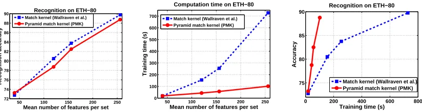
In fact, the ability of a kernel to handle large numbers of features can be critical to its success. An interest operator may be tuned to select only the most salient features, but in our experiments we found that recognition rates always benefited from having larger numbers of features per image with which to judge similarity. The plots in Figure 6 depict the run-time versus recognition accuracy of the pyramid match kernel as compared to the match kernel (Wallraven et al., 2003), which has

O(dm2) complexity. The match kernel computes kernel values by averaging over the distances between every point in one set and its nearest point in the other set. These are results from our own implementation of the match kernel. Each point in the figure represents one experiment, and both kernels were run with the exact same PCA-SIFT feature sets. The saliency threshold of the Harris interest operator was adjusted to generate varying numbers of features, thus trading off accuracy versus run-time. With no filtering of the Harris detector output (i.e., with a threshold of 0), there is on average 153 features per set. To extract an average of 256 features per set we used no interest operator and sampled features densely and uniformly from the images. Computing a kernel matrix for the same data with the two kernels yields nearly identical accuracy (left plot), but the pyramid match is significantly faster (center plot). Allowing the same amount of training time for both methods, the pyramid match produces much better recognition results (right plot).

9.2 Caltech-101 Data Set

We also tested our method with a challenging database of 101 object categories developed at Cal-tech, called the Caltech-101 (Fei-Fei et al., 2004). The creators of this database obtained the images

50 100 150 200 250 72

74 76 78 80 82 84 86 88

90 Recognition on ETH−80

Mean number of features per set

Recognition accuracy

Match kernel (Wallraven et al.) Pyramid match kernel (PMK)

50 100 150 200 250

0 100 200 300 400 500 600 700

Computation time on ETH−80

Mean number of features per set

Training time (s)

Match kernel (Wallraven et al.) Pyramid match kernel (PMK)

0 200 400 600 800

75 80 85 90

Training time (s)

Accuracy

Recognition on ETH−80

Match kernel (Wallraven et al.) Pyramid match kernel (PMK)

Figure 6: Both the pyramid match kernel and the match kernel of Wallraven et al. yield comparable recognition accuracy for input sets of the same size (left plot). Both benefit from using richer (larger) image descriptions. However, while the time required to learn object cat-egories with the quadratic-time match kernel grows quickly with the input size, the time required by the linear-time pyramid match remains very efficient (center plot). Allowing the same run-time, the pyramid match kernel produces better recognition rates than the match kernel (right plot). Recognition accuracy is measured as the mean rate of correct predictions per class.

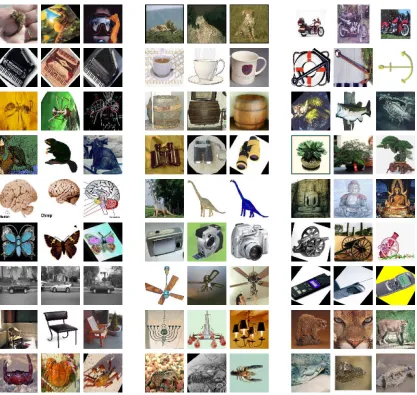
using Google Image Search, and many of the images contain a significant amount of intra-class ap-pearance variation (see Figure 7). The Caltech-101 is currently the largest benchmark recognition data set (in terms of number of categories) available, and as such it has been the subject of many recent recognition experiments in the field. There are 8677 images in the data set, with between 31 to 800 images for each of the 101 categories.

For this data set, the pyramid match operated on sets of SIFT features projected to d =10 dimensions using PCA, with each appearance descriptor concatenated with its corresponding posi-tional feature (image position normalized by image dimensions). The features were extracted on a uniform grid at every 8 pixels in the images, that is, no interest operator was applied. The regions extracted for the SIFT descriptor were about 16 pixels in diameter, and each set had on average

m=1140 features. We trained the algorithm using unsegmented images. Since the pyramid match seeks a strong correspondence with some subset of the images’ features, it explicitly accounts for unsegmented, cluttered data. Classification was again done with a one-vs-all SVM, and we set the number of grid shifts T =1, and summed over kernels corresponding to pyramids with finest side lengths of 5,7, and 9. Note that some images were rotated by the creators of the database, causing some triangular artifacts in the corners of some images; this is how the images are provided to any user.

As a baseline, we also experimented with the bag-of-words representation and an RBF kernel:

Figure 7: Example images from the Caltech-101 database. Three images are shown for each of 27 of the 101 categories.

feature prototypes (“words”) was tested at values ranging from 1000 to 100,000 (2200 was best); the kernel’sσparameter was tested from values of 500 to 10,000 (1000 was best).

per-formance with any number of training examples would be just 1%. Using 15 examples (a standard point of comparison), the pyramid match achieves an average recognition rate per class of 50%. Experiments comparing the recognition accuracy of the pyramid match kernel to an optimal partial matching kernel reveal that very little loss in accuracy is traded for speedup factors of several orders of magnitude (Grauman, 2006, , pages 118-121).

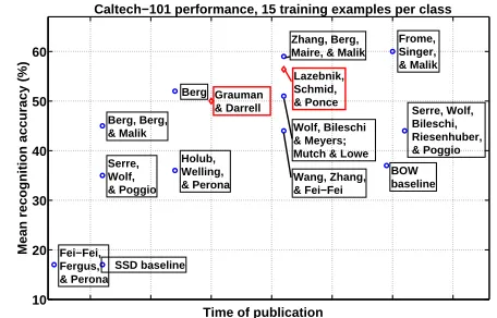
Over all the parameter configurations we tested, the best performance we could achieve with the bag-of-words on this data set is substantially poorer than that of the pyramid match, as seen in Figure 8 (a). In addition, the bag-of-word approach’s accuracy was fairly sensitive to the parameter settings; for instance, over all the parameters we tested, the mean accuracy for 15 training examples per class varied from 28% to 37%. This indicates the difficulty of establishing an optimal flat quantization of the feature space for recognition, and also suggests that the partial matching ability of the pyramid match is beneficial for tolerating outlier features without skewing the matching cost.

Figure 8 (b) shows all published results on this data set as a function of time since the data was released, including the PMK and results published more recently by other authors (Holub et al. 2005b; Serre et al. 2007; Wolf et al. 2006; Wang et al. 2006; Berg et al. 2005; Berg 2005; Fei-Fei et al. 2004; Mutch and Lowe 2006; Lazebnik et al. 2006; Zhang et al. 2006; Frome et al. 2007). From this comparison we can see that even with its extreme computational efficiency, the pyramid match kernel achieves results that are competitive with the state-of-the-art. We have pre-viously obtained 50% accuracy on average (0.9% standard deviation) when using the standard 15 training examples per category (Grauman and Darrell, 2006). In addition, the PMK with sets of spatial features yields very good accuracy on this data set: 56.4% for 15 training examples per class (Lazebnik et al., 2006). These results are based on a special case of the pyramid match, where mul-tiple pyramid match kernels computed on spatial features are summed over a number of quantized appearance feature channels. This is among the very best accuracy rates reported to-date on the data set, and about three percentage points below the most accurate result of 60% obtained recently by Frome et al. (2007), which compares images using a discriminative local distance function.

Figure 8 (c) shows the recognition accuracy of various methods as a function of computation time, measured in terms of the time required to train a classifier (left plot) and the time required to classify a novel example (right plot). We collected these time estimates directly from the au-thors, and every response we received is plotted here. (So not every method represented in (b) is represented in (c) due to a lack of information on computation times.) For both plots in part (c), computation time is measured excluding the time required to extract image features for all methods. For display purposes, in the left plot, we plot the square root of the training time; nearest-neighbor classifiers such as the method of Berg et al. require no training time beyond feature extraction. In the right plot, we plot the log of the classification time estimates to reflect the relative complexities in terms of orders of magnitude. This figure illustrates the PMK’s clear practical cost advantages. Pyramid matching any two examples requires just 0.0001 s on this data set, and classifying a novel example requires a fraction of a second; in contrast, many other techniques require on the order of a minute to classify a single example, and yield varying accuracies relative to the PMK.