Unlabeled Compression Schemes for Maximum Classes
∗Dima Kuzmin [email protected]
Manfred K. Warmuth [email protected]
Computer Science Department University of California, Santa Cruz 1156 High Street
Santa Cruz, CA, 95064
Editor: John Shawe-Taylor
Abstract
Maximum concept classes of VC dimension d over n domain points have size ≤nd, and this is an upper bound on the size of any concept class of VC dimension d over n points. We give a compression scheme for any maximum class that represents each concept by a subset of up to d unlabeled domain points and has the property that for any sample of a concept in the class, the representative of exactly one of the concepts consistent with the sample is a subset of the domain of the sample. This allows us to compress any sample of a concept in the class to a subset of up to d unlabeled sample points such that this subset represents a concept consistent with the entire original sample. Unlike the previously known compression scheme for maximum classes (Floyd and Warmuth, 1995) which compresses to labeled subsets of the sample of size equal d, our new scheme is tight in the sense that the number of possible unlabeled compression sets of size at most d equals the number of concepts in the class.
Keywords: compression schemes, VC dimension, maximum classes, one-inclusion graph
1. Introduction
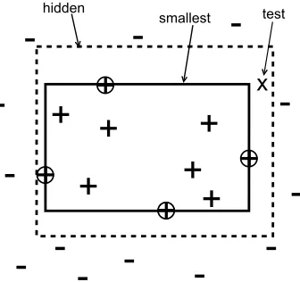
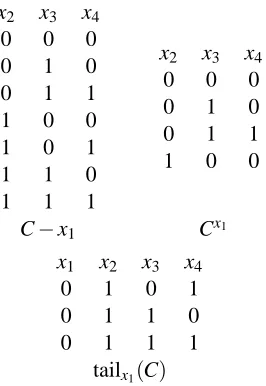
Consider the following type of protocol between a learner and a teacher. Both agree on a domain and a class of concepts (subsets of the domain). For instance, the domain could be the plane and a concept the subset defined by an axis-parallel rectangle (see Figure 1). The teacher gives a set of training examples (labeled domain points) to the learner. The labels of this set are consistent with a concept (rectangle) that is hidden from the learner. The learner’s task is to predict the label of the hidden concept on a new test point.
Intuitively, if the training and test points are drawn from some fixed distribution, then the la-bels of the test point can be predicted accurately provided the number of training examples is large enough. The sample size should grow with the inverse of the desired accuracy and with the com-plexity or “dimension” of the concept class. The most basic notion of dimension in this context is the Vapnik-Chervonenkis dimension. This dimension is the size d of the maximum cardinality subset of domain points such that all 2d labeling patterns can be realized by a concept in the class. The VC dimension of axis-parallel rectangles is 4, since it is possible to label any set of 4 points in all possible ways as long as no point lies inside the orthogonal hull of the other 3 points (where
+
+
+
+
+
--
-x
+
+
+
+
+
hidden
smallest test
Figure 1: An example set consistent with some axis-parallel rectangle. Also shown is the smallest axis-parallel rectangle containing the subsample of circled points. This rectangle is con-sistent with all examples and the set of circled points represents a concon-sistent concept. The hidden rectangle generating the data is dashed. “x” is the next test point.
the orthogonal hull is defined as the smallest rectangle containing the points); also for any 5 points, at least one of the points lies inside the orthogonal hull containing the remaining 4 points and this disallows at least one of the 25patterns.
This paper deals with an alternate notion of dimension used in machine learning that is related to compression (Littlestone and Warmuth, 1986). It stems from the observation that you can often select a subset of the training examples to represent a hypothesis consistent with all training exam-ples. For instance, in the case of rectangles, it is sufficient to keep only the uppermost, lowermost, leftmost and rightmost positive point. There are up to 4 points in the subsample (since some of the 4 extreme points might coincide.) The orthogonal hull of the subsample will always be consistent with the entire sample.
More generally, a compression scheme is defined by two mappings (Littlestone and Warmuth, 1986): one mapping samples of concepts in the class to subsamples, and the other one mapping the resulting subsamples to hypotheses on the domain of the class. Compression schemes must have the property that the subsample always represents a hypothesis consistent with the entire original sample. However note that the reconstructed hypothesis doesn’t have to lie in the original concept class. It only needs to be consistent with the original sample. The subsamples represent hypotheses and are called representatives in this paper. A compression scheme can be viewed as a set of rep-resentatives of hypotheses with the property that every sample of the class contains a representative of a consistent hypothesis. The size of the compression scheme is the size of the largest represen-tative, and the minimum size of a compression scheme for a class serves as an alternate measure of complexity.
The size of the compression scheme also replaces the VC dimension in the PAC sample size bounds (Littlestone and Warmuth, 1986; Floyd and Warmuth, 1995; Langford, 2005). However, in the case of compression schemes, the proofs of these bounds are much simpler. There are many practical algorithms based on compression schemes (e.g., Marchand and Shawe-Taylor, 2002, 2003). Also, any algorithm with a mistake bound M leads to a compression scheme of size M (Floyd and Warmuth, 1995).
Let’s consider some more illustrative examples of compression schemes. Unions of up to k intervals on the real line form a concept class of VC dimension 2k. We can compress a sample from this class to the following set of points: the leftmost “+” point in the sample, the leftmost “−” point to the right of the last selected point, the leftmost “+” further to the right of the last selected point, and so forth; stop when there are no more points whose label is opposite to the last selected point. It is easy to see that at most 2k points are kept when the original sample is consistent with a union of k intervals. Also the labels of the entire original sample can be reconstructed from this subsample. Note that in this case the labels of the subsample are always alternating starting with a “+”. Thus these labels are redundant and the above scheme can be interpreted as compressing to unlabeled subsamples of size at most the VC dimension 2k.
Support Vector Machines also lead to a simple labeled compression scheme for halfspaces (sets of the form{x∈Rn:w·x≥b}), because only the set of support vectors is needed to reconstruct
the hyperplane consistent with the original sample. Of course, the number of support vectors can be quite big. However, it suffices to keep any set of essential support vectors and these sets have size n+1, where n is the dimension of the feature space (von Luxburg et al., 2004). Not surprisingly, n+1 is also the VC dimension of arbitrary halfspaces of dimension n. However, the labels of a set of essential support vectors are not redundant and this provides an example of a labeled compression scheme for halfspaces. There also exists a compression scheme for the same class that compresses to at most n+1 unlabeled points (Ben-David and Litman, 1998). However this scheme is not constructive.
The compression scheme conjecture is easily proven for intersection-closed concept classes (Helmbold et al., 1992), which include the class of axis-parallel rectangles as a special case. More importantly, the conjecture was shown to be true for maximum classes. A finite class of VC dimen-sion d over n domain points is maximum if its size is equal to ≤nd, which is the upper bound on the size of any concept class of VC dimension d over n points. An infinite class of VC dimension d is maximum if all restrictions to a finite subset of domain of size at least d are maximum classes of dimension d.
Of the example concept classes discussed so far, the class of up to k intervals on the real line is maximum. The class of halfspaces inRnis not maximum, but it is in fact a union of two classes of
VC dimension n which are “almost maximum”: positive halfspaces and negative halfspaces (Floyd, 1989). Positive halfspaces are those that contain the “point”(∞,0, . . . ,0)and negative halfspaces are those that contain(−∞,0, . . . ,0). Both classes of halfspaces are almost maximum in the sense that the restriction to any set of points in general position always produces a maximum class. Finally, the class of axis-parallel rectangles is not maximum since for any five points at least two labelings are not realizable.
com-x1 x2 x3 x4 r(c)
c1 0 0 0 0 /0
c2 0 0 1 0 {x3}
c3 0 0 1 1 {x4}
c4 0 1 0 0 {x2}
c5 0 1 0 1 {x3,x4}
c6 0 1 1 0 {x2,x3}
c7 0 1 1 1 {x2,x4}
c8 1 0 0 0 {x1}
c9 1 0 1 0 {x1,x3}
c10 1 0 1 1 {x1,x4}
c11 1 1 0 0 {x1,x2}
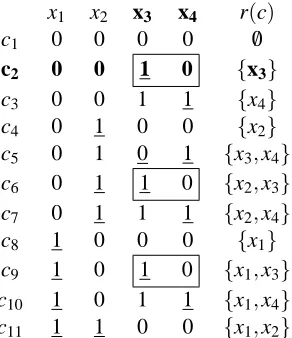
Figure 2: Illustration of the unlabeled compression scheme for some maximum concept class. The representatives for each concept are indicated in the right column and also as the under-lined positions in each row. Suppose the sample is x3=1,x4=0. The set of concepts
consistent with that sample is {c2,c6,c9}. The representative of exactly one of these
concepts is entirely contained in the sample domain{x3,x4}. For our sample this
repre-sentative is{x3}which represents c2. So the compressed sample becomes{x3}.
presses any sample consistent with a concept to at most d unlabeled points from the sample. If m is the size of the sample, then there are ≤mdsets of points of size up to d. For maximum classes, the number of different labelings induced on any set of size m is also ≤md. Thus our new scheme is “tight”. In the previous labeled scheme, the number of possible representatives was much bigger than the number of concepts.
The new unlabeled scheme also has many interesting combinatorial properties. Let us represent finite classes as a binary table (see Figure 2) where the rows are concepts and the columns are all the points in the domain. Our compression scheme represents concepts by subsets of size at most d and for any k≤d, the concepts represented by subsets of size up to k will form a maximum class of VC dimension k. Our scheme compresses as follows: After receiving a set of examples, we first restrict ourselves to concepts that are consistent with the sample. We then compress to a representative of a consistent concept that is completely contained in the sample domain (see Figure 2). As our main result we will prove that for our choice of representatives, for any sample there always will be exactly one of the consistent concepts whose representative is completely contained in the sample domain.
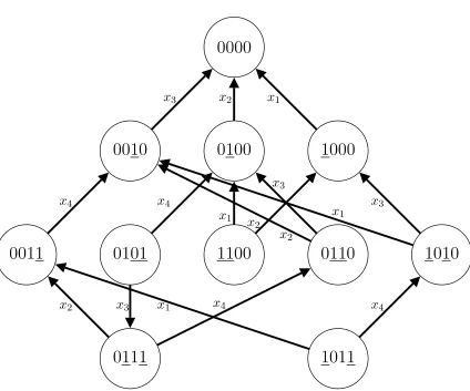
Our new unlabeled compression scheme is connected to a certain undirected graph, called the one-inclusion graph, that characterizes the concept class on a set of example points (Haussler et al., 1994): the vertices are the possible labelings of the example points and there is an edge between two concepts if they disagree on a single point. The edges are naturally labeled by the differing points (see Figure 4).
Any prediction algorithm can be used to orient the edges of the one-inclusion graphs as follows. Assume we are given a labeling of some m points x1, . . . ,xmand an unlabeled test point x. If there
x1 x2 x3 x4
c1 0 0 1 0
c2 0 1 0 0
c3 0 1 1 0
c4 1 0 1 0
c5 1 1 0 0
c6 1 1 1 0
c7 0 0 1 1
c8 0 1 0 1
c9 1 0 0 0
c10 1 0 0 1
,
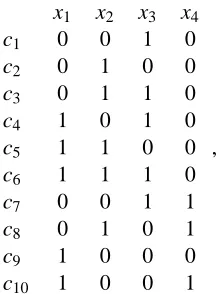
Figure 3: A maximal class of VCdim 2 with 10 concepts. Maximum concept classes of VCdim 2 have ≤42=11 concepts (see Figure 2).
one-inclusion graph for the set{x1, . . . ,xm,x}. This edge connects the two possible extensions of
the labeling of x1, . . . ,xmto the test point x. If the algorithm predicts b, then orient the edge toward
the concept that labels x with bit b.
The vertices in the one-inclusion graph represent the possible labelings of {x1, . . . ,xm,x}
pro-duced by the target concepts and if the prediction is averaged over all permutations of the m+1 points, then the probability of predicting wrong is md+1, where d is the out-degree of the target. Therefore the canonical optimal algorithm predicts with an orientation of the one-inclusion graphs that minimizes the maximum out-degree (Haussler et al., 1994; Li et al., 2002) and in Haussler et al. (1994) it was shown that this outdegree is at most the VC dimension.
How is this all related to our new compression scheme for maximum classes? We show that for any edge labeled with x, exactly one of the two representatives of the incident concepts contains the point x. Thus by orienting the edges toward concept that does not have x, we immediately obtain an orientation of the one-inclusion graphs in which all vertices have maximum outdegree at most d (which is the best possible). Again such a d-orientation immediately leads to prediction algorithms with a worst case expected mistake bound of m+d1, where m is the sample size (Haussler et al., 1994), and this bound is optimal1(Li et al., 2002).
The conjecture whether there always exists a compression scheme of size at most the VC di-mension remains open. For finite domains it clearly suffices to resolve the conjecture for maximal classes (i.e., classes where adding any concept would increase the VC dimension). We do not know of any natural example of a maximal concept class that is not maximum or closely related. However, it is easy to find small artificial maximal classes (see Figure 3). We believe that much of the new methodology developed in this paper for maximum classes will be useful in deciding the general conjecture in the positive and think that in this paper we made considerable progress toward this goal. In particular, we developed a refined recursive structure of finite concept classes and made the connection to orientations of the one-inclusion graphs. Also, our scheme constructs a certain unique matching that is interesting in its own right.
Even though the unlabeled compression schemes for maximum classes are tight in some sense, they are not unique. There is a strikingly simple “peeling algorithm” that always seems to produce a valid unlabeled compression scheme for maximum classes: construct the one-inclusion graph for the domain; iteratively peel off a lowest degree vertex and represent a concept c by the set of data points incident to vertex c in the remaining graph when c was removed from the graph (see Figure 7 for an example run). However, we have no proof of correctness of this algorithm and the resulting schemes do not have as much recursive structure as the ones produced by our recursive algorithm for which we have correctness proof. For the small example given in Figure 2, both algorithms can produce the same scheme.
1.1 Outline of the Paper
Some basic definitions are provided in Section 2. We then define unlabeled compression schemes in Section 3 and characterize the properties of the representation mappings of such schemes and their relation to the one-inclusion graph. In this section we also discuss the simple Min-Peeling Al-gorithm in more detail. This alAl-gorithm always seems to provide an unlabeled compression scheme even though we currently do not have a correctness proof for it. Section 4 discusses linear ar-rangements, which are special maximum concept classes, and discuss how to interpret unlabeled compression schemes for these classes. Next, in Section 5, we briefly summarize the old scheme for maximum classes from Floyd and Warmuth (1995) which compresses to labeled subsamples, whereas ours uses unlabeled ones. The core of the paper is in Section 6, where we give a recursive algorithm for constructing an unlabeled compression scheme with a detailed proof of correctness. Section 7 contains additional combinatorial lemmas about the structure of maximum classes and unlabeled compression schemes. In Section 8, we discuss how to possibly extend various compres-sion schemes for maximum classes to the more general case of maximal classes. We conclude in Section 9 with a large number of combinatorial open problems that we have encountered in this research.
2. Definitions
Let X be a domain, where we allow X=/0. A concept c is a mapping from X to{0,1}. We can also view a concept c as a characteristic function of a subset of dom(c), that is, for any domain point x∈dom(c), c(x) =1 iff x∈c. A concept class C is a set of concepts with the same domain (denoted as dom(C)). Such a class is represented by a binary table (see Figure 2), where the rows correspond to concepts and the columns to points in dom(C).
Alternatively, C can be represented as a subgraph of the Boolean hypercube of dimension
|dom(C)|. Each dimension corresponds to a particular domain point, the vertices are the concepts in C and two concepts are connected with an edge if they disagree on the label of a single point. This graph is called the one-inclusion graph of C (Haussler et al., 1994). Note that each edge is naturally labeled by the single dimension/point on which the incident concepts disagree (see Figure 4). The set of incident dimensions of a vertex c in a one-inclusion graph G is the set of dimensions labeling the edges incident to c. We denote this set as IG(c). Its size equals the degree of c in G.
0000
0010
0011
0100
0101
0110
0111
1000
1010
1011
1100
x
3x
2x
1x
4x
1x
2x
1x
4x
3x
1x
3x
4x
3x
2x
4x
2x2 x3 x4
0 0 0
0 1 0
0 1 1
1 0 0
1 0 1
1 1 0
1 1 1
x2 x3 x4
0 0 0
0 1 0
0 1 1
1 0 0
C−x1 Cx1
x1 x2 x3 x4
0 1 0 1
0 1 1 0
0 1 1 1
tailx1(C)
Figure 5: The reduction, restriction and the tail of the concept class from Figure 2 wrt x1.
identical rows.2 Also the one-inclusion graph for the restriction C|A is now a subgraph of the Boolean hypercube of dimension|A|instead of the full dimension|C|. We use c−x as shorthand for c|(dom(C)r{x})and let C−x denote{c−x|c∈C}(produced by removing column x from the
table, see Figure 5). A sample of a concept c is any restriction c|A for some A⊆dom(c).
The reduction Cxof a concept class C wrt a dimension x∈dom(C)consists of all those concepts
in C−x that have two possible extensions onto concepts in C. All such concepts correspond to an edge labeled with x in the one-inclusion graph (see Figure 5). In summary, the class Cx is a subset of C−x that has the same reduced domain X− {x}.
The tail of concept class C on dimension x consists of all concepts that do not have an edge labeled with x. Thus it corresponds to the subset of C−x that has a unique extension onto the full domain. We denote the tail of C on dimension x as tailx(C). The class C can therefore be partitioned
as 0Cx∪1Cx∪ tailx(C), where
∪denotes the disjoint union and bCx consists of all concepts in Cx extended with bit b in dimension x. Note that tails have the same domain as the original class, whereas the reduction and restriction are classes that have a reduced domain.
A finite set of dimensions A⊆dom(C) is shattered by a concept class C if for any possible labeling of A, the class C contains a concept consistent with that labeling (i.e., size(C|A) =2|A|).3 The Vapnik-Chervonenkis dimension of a concept class C is the size of a maximum subset that is shattered by that class (Vapnik, 1982). We denote this dimension as VCdim(C). Note that if|C|=1, then VCdim(C) =0.4
In this paper we use the binomial coefficients nd, for integers n≥0 and d, where nd=0 for d >n or d <0 and 00=1. We make use of the following identity which holds for n>0:
n d
= n−d1+ nd−−11. Let ≤nd be a shorthand for the binomial sums∑di=0 ni. Then we have a similar identity for the binomial sums when n>0: ≤nd= n≤−d1+ ≤nd−−11.
From Vapnik and Chervonenkis (1971) and Sauer (1972) we know that for all concept classes with VC dimension d:|C| ≤ |dom≤d(C)|(generally known as Sauer’s lemma). A concept class C with VCdim(C) =d is called maximum (Welzl, 1987) if for all finite subsets Y of the domain dom(C), size(C|Y) = ≤|Yd|. If C is a maximum class with d=VCdim(C), then∀x∈dom(C), the classes C−x and Cxare also maximum classes and have VC dimensions d and d−1, respectively (Welzl, 1987). From this it follows that for finite domains, a concept class C is maximum iff size(C) = |dom≤(dC)|.
A concept class C is called maximal if adding any other concept to C will increase its VC dimension. Any maximum class on a finite domain is also maximal (Welzl, 1987). However, there exist finite maximal classes, which are not maximum (see Figure 3 for an example).
From now on we only consider finite classes. As our main result we construct an unlabeled compression scheme for any finite maximum class. The existence of an unlabeled scheme for infinite maximum classes then follows from a compactness theorem given in Ben-David and Litman (1998). The proof of that theorem is, however, non-constructive.
3. Unlabeled Compression Scheme
Our unlabeled compression scheme for maximum classes represents the concepts as unlabeled sub-sets of dom(C) of size at most d. For any c∈C we call r(c) its representative. Intuitively we want concepts to disagree on their representatives. We say that two different concepts clash wrt r if c|(r(c)∪r(c0)) =c0|(r(c)∪r(c0)).
Main definition: A representation mapping r of a maximum concept class C must have the follow-ing two properties:
1. r is a bijection between C and (unlabeled) subsets of dom(C)of size at most VCdim(C)and
2. no two concepts in C clash wrt r.
The following lemma shows how the non-clashing requirement can be used to find a unique repre-sentative for each sample.
Lemma 1 Let r be any bijection between a finite maximum concept class C of VC dimension d and subsets of dom(C)of size at most d. Then the following two statements are equivalent:
1. No two concepts clash wrt r.
2. For all samples s of a concept from C, there is exactly one concept c∈C that is consistent with s and r(c)⊆dom(s).
Based on this lemma it is easy to see that a representation mapping r for a maximum concept class C defines a compression scheme as follows. For any sample s of C we compress s to the unique representative r(c) such that c is consistent with s and r(c)⊆dom(s). Reconstruction is even simpler, since r is bijective: if s is compressed to the set r(c), then we reconstruct to the concept c. See Figure 2 for an example of how compression and reconstruction work.
Proof of Lemma 1
1⇒2 : At a high level, for any sample domain dom(s) there are as many representatives r(c)⊆
dom(s)as there are different samples having that domain. The no clashing condition implies that all concepts with representatives in dom(s)are different from each other on dom(s), thus every sample has to get at least one representative.
For a more detailed proof assume¬2, that is, there is a sample s for which there are either zero or (at least) two consistent concepts c for which r(c)⊆dom(s). If two concepts c,c0∈C are consistent with s and r(c),r(c0)⊆dom(s), then c|r(c)∪r(c0) =c0|r(c)∪r(c0) (which is
¬1). If there is no concept c consistent with s for which r(c)⊆dom(s), then since
size(C|dom(s)) =
|dom(s)| ≤d
=|{c : r(c)⊆dom(s)}| .
there must be another sample s0with dom(s0) =dom(s)for which there are two such concepts.
So again¬1 is implied. 2
Once we have a valid representation mapping for some maximum concept class C, we can easily derive a valid mapping for any restriction of the class C|A by compressing every restricted concept. This is discussed in the following corollary.
Corollary 2 For any maximum class C and A⊆dom(C), if r is a representation mapping for C then a representation mapping for C|A can be constructed as follows. For any c∈C|A, let rA(c)be
the representative of the unique concept c0∈C, such that c0|A=c and r(c0)⊆A.
Proof The construction of the mapping for C|A essentially tells us to treat the concept c as a sample from C and to compress it. Thus we can apply Lemma 1 to see that rA(c)⊆A is always uniquely
de-fined. Now we need to show that rAsatisfies the conditions of the Main Definition. Since the
repre-sentatives rA(c)are subsets of A, the non-clashing property for the representation mapping rAfor C|A
follows from the non-clashing condition for r for C. The bijection property follows from a counting argument like the one used in the proof of Lemma 1, since size(C|A) =size({r(c)s.t. r(c)⊆A}).
The following lemmas and corollaries will be stated only for the concept class C itself. However, in light of Corollary 2 they will also hold for all restrictions C|A.
We first show that a representation mapping r for a maximum classes can be used to derive a d-orientation for the one-inclusion graph of the class (i.e., an orientation of the edges such that the outdegree of every vertex is at most d). As discussed in the introduction such orientations lead to a prediction algorithm with a worst-case expected mistake bound of dt at trial t.
Lemma 3 For any representation mapping r of a maximum concept class C and the one-inclusion graph of C, any edge c— cx 0 in the graph has the property that its associated dimension x lies in exactly one of the representatives r(c)or r(c0).
Proof Since c and c0differ only on dimension x and c|r(c)∪r(c0)=6 c0|r(c)∪r(c0), x lies in at least one of r(c),r(c0). Next we will show that x lies in exactly one.
and upper bounded by the total size of all representations. We complete the proof of the lemma by showing that the number of edges equals the total size of all representatives. This means that no edge can charge both of its incident concepts and each point labeling an edge must lie in exactly one of the representations of its incident concepts.
There are |Cx|edges labeled with dimension x in the one-inclusion graph for C. Since there are n dimensions and Cxis always maximum and of dimension d−1, the total number of edges in the graph is n ≤nd−−11, where n=|dom(C)|, d=VCdim(C). (This formula is also a special case of Lemma 15.) The total size of all representatives is the same number because:
∑
c∈C
|r(c)|=
d
∑
i=0
i
n i
=n
d
∑
i=1
n−1
i−1
=n
n−1
≤d−1
.
The above lemma lets us orient the one-inclusion graphs for the class.
Corollary 4 For any representation mapping of maximum class C and the one-inclusion graph of C, directing each edge away from the concept whose representative contains the dimension of the edge creates a d-orientation of the one-inclusion graph for the class.
Proof The outdegree of every concept is equal to size of its representative, which is≤d.
The lemma also implies that the representatives of concepts are always subsets of the set of incident dimensions in the one-inclusion graphs.
Corollary 5 Any representation mapping r of a maximum class C has the property that for any concept c∈C, its representative r(c)is a subset of the dimensions incident to c in the one-inclusion graph for C.
Proof From the counting argument in the proof of Lemma 3 we see that for every x∈r(c) there must exist an edge leaving c in the graph labeled with x.
3.1 The Min-Peeling Algorithm
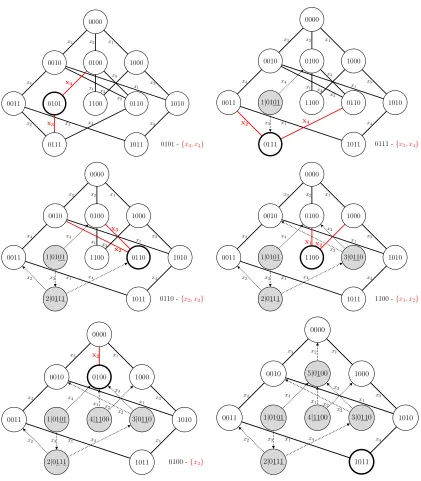
As discussed at the end of the introduction, there is a simple algorithm that always seems to construct a correct representation mapping for any maximum class. The algorithm iteratively removes any lowest degree vertex from the one-inclusion graph for the remaining class and sets the representative r(c) to the set of dimensions of the edges incident to c when c was removed from the graph. The algorithm is formally stated in Figure 6. An illustration of several iterations of the algorithm is given in Figure 7.
Min-Peeling Algorithm
Input: a finite maximum concept class C. Output: a representation mapping r for C Let G be the one-inclusion graph for C
While C6=/0
1. Choose a minimum-degree vertex c among those in C
2. r(c):=set of dimension incident to c in the graph
3. Remove c from G and C
Figure 6: The Min-Peeling Algorithm for constructing an unlabeled compression scheme for max-imum classes.
thus it does not contradict the Min-Peeling Algorithm. Maximum classes and classes obtained by peeling them appear to have a special structure that always ensures existence of a degree≤d vertex, where d is the VC dimension of the remaining class. However a complete proof of this statement needs to be found.
The representation mappings produced by the Min-Peeling Algorithm have less structure than the representation mappings produced by the Tail Matching Algorithm discussed in Section 6. In particular, they do not necessarily satisfy the condition of Lemma 12, which states the subset of concepts corresponding to representations of size up to k forms a maximum class of VC dimension k. For the maximum class of Figure 2, both algorithms can produce the same representation mapping. Also note how the Min-Peeling Algorithm immediately leads to a d-orientation of the one-inclusion graph: as we peel away a vertex, its edges are naturally oriented away from the vertex before the edges are removed. Since each vertex has degree at most d when it is peeled away, the outdegree of each vertex will be at most d. Moreover, the resulting orientation of the one-inclusion graph is acyclic because all edges are oriented from a vertex toward a vertex that is removed later. In other words, the list of vertices produced by the Min-Peeling Algorithm is a topological ordering of the oriented one-inclusion graph (see Figure 8). As we shall see later, the Tail Matching Algo-rithm also produces a topological order of the graph. By Corollary 4, every representation mapping induces a d-orientation of the one-inclusion graph. However we found examples where a valid representation mapping for a maximum class induces a cyclic orientation (not shown).
4. Linear Arrangements
In this section we visualize many of our basic notations and unlabeled compression schemes for simple linear arrangements, which are special maximum classes. An unlabeled compression scheme for linear arrangements is also described in Ben-David and Litman (1998).
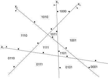
A linear arrangement is a collection of oriented hyperplanes inRd. The cells of the arrangement
0000 0010 0011 0100 0101 0110 0111 1000 1010 1011 1100
x3 x2 x1
x4 x1 x2 x1 x4 x3 x1
x3 x4
x3 x2
x4 x2
0101 -{x3, x4}
0000
0010
0011
0100
1|0101 0110
0111
1000
1010
1011 1100
x3 x2 x1
x4
x1
x2 x1
x4
x3
x1
x3 x4
x3
x2
x4 x2
0111 -{x2, x4}
0000
0010
0011
0100
1|0101 0110
2|0111
1000
1010
1011 1100
x3 x2 x1
x4 x1 x2 x1 x4 x3 x1 x3 x4 x3 x2 x4 x2
0110 -{x2, x3}
0000
0010
0011
0100
1|0101 3|0110
2|0111
1000
1010
1011 1100
x3 x2 x1
x4
x1
x2 x1
x4
x3
x1
x3 x4
x3
x2
x4
x2
1100 -{x1, x2}
0000
0010
0011
0100
1|0101 3|0110
2|0111
1000
1010
1011 4|1100
x3 x2 x1
x4
x1
x2 x1
x4
x3
x1
x3 x4
x3
x2
x4
x2
0100 -{x
2}
0000
0010
0011
5|0100
1|0101 3|0110
2|0111
1000
1010
1011 4|1100
x3 x2 x1
x4
x1
x2 x1
x4
x3
x1
x3 x4
x3
x2
x4
x2
Figure 8: Topological order and d-orientation produced by a run of Min-Peeling Algorithm for some maximum class.
x1
x3
x4
1010
1110
0110
0111
0101 1101 1000
1001
0001 1011
1111
x2
Figure 9: An example linear arrangement. The cells of the arrangement represent the concepts and the planes the dimensions of the class. All cells on the upper side of a hyperplane (indicated by an arrow) are labeled one in the corresponding dimension and the cells on the lower side are labeled zero. Up to d hyperplanes bordering a cell are marked and the set of dimensions of these marked planes forms the representative of the cell in the unlabeled compression scheme.
x
1
x
2
x3
1010
1110
0110
0111
0101
1101
1000
1001
0001
1011
1111
x4
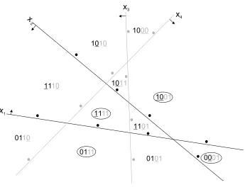
Figure 10: Restriction C−{x3,x4}of the linear arrangements concept class of Figure 9. The planes
x3 and x4 are grayed. Several cells of the full arrangement are combined into bigger
cells of the restricted arrangement. One of the subcells forming each big cell (circled) has the property that all dimensions in its representative are still available (none of the corresponding hyperplanes were grayed). The representative of this subcell represents the big cell. For example the subcells 1110,1111,1101 form the larger cell for sample
(x1,1),(x2,1) and only 1111 (circled) is represented by a subset of non-grayed
hyper-planes: r(1111) ={x1}, and therefore the sample is compressed to{x1}.
common) then the arrangement is called simple. Such arrangements are maximum classes because their VC dimension is min{n,d}and they have ≤nd cells (Edelsbrunner, 1987). However not all finite maximum classes are representable as linear arrangements (Floyd, 1989).
The vertices of the one-inclusion graph are the cells of the arrangement and edges connect neighboring cells. A restriction C−x corresponds to removing the x plane from the arrangement. Pairs of cells that border this plane are now combined to larger cells (an example of a double restric-tion is given in Figure 10). Samples are combined cells produced by removing some hyperplanes. The reduction Cx is the arrangement in the space of dimension d−1 induced by the projection of
the remaining n−1 planes onto the x plane. The subclasses 1Cxand 0Cxcorrespond to the cells di-rectly above or below the x plane, respectively. All cells not bordering the x plane form the subclass tailx(C).
neighbouring cells (See Figure 9). Each cell marks at most d bordering hyperplanes and no cell marks the same set of hyperplanes. The no-clashing condition of our Main Definition means that any two cells are on opposite sides of at least one hyperplane marked by one of the cells. Also by Lemma 3, any boundary shared between any two cells is marked on exactly one side.
We now visualize how we compress a sample, that is, we restate the process described in Figure 2 for the special case of linear arrangements. Recall that a sample s corresponds to a combined cell produced by removing the hyperplanes in dom(c)rdom(s) where each of the original cells
corresponds to a concept consistent with the sample. One (and only one) of the original cells in the combined cell that corresponds to the sample is marking only hyperplanes from the surviving set dom(s)(circled in Figure 10). We compress the sample to that set of marked dimensions and reconstruct based on the represented original cell. Note that if the selected original cell marks any plane, then it must always be at the boundary of the combined cell, since cells in the middle do not border any of the remaining hyperplanes.
It is interesting to observe how our algorithms construct representation mappings for linear arrangements.
Conjecture 1. Sweeping the arrangement with a hyperplane that is not parallel to any plane in the arrangement produces a compression scheme as follows: as soon as a cell is completely swept, it marks the planes of all bordering currently live cells. The resulting sequential assignments of representatives to concepts corresponds to a run of the Min-Peeling Algorithm.
In particular we conjecture that sweeping as prescribed iteratively completes minimum degree cells.
The recursive Tail Matching Algorithm of Section 6 chooses some plane x and first finds a compression scheme for the projection Cx of the linear arrangement onto the this plane. Each projected cell from Cx corresponds to two cells, one from 0Cx and one from 1Cx. The algorithm uses the scheme for Cx for all concepts in 0Cx, that is, all cells bordering the x plane from below. The sibling cells in 1Cx right above the plane receive the same marks but also an additional mark from the x plane. The recursive algorithm uses exactly d marks for all vertices in tailx(C)(the cells
not bordering the x plane). However, this assignment cannot be easily visualized.
Note that one of the planes has the property that the markings produced by the recursive algo-rithm all lie on one side of the plane. We initially conjectured that there always exist representation schemes that place the marks on the same side for all planes. However we found small counterex-amples to this conjecture (not shown).
Simple linear arrangements are known to have the following property: the shortest path between any two cells is always equal to the Hamming distance between the cells (Edelsbrunner, 1987). Surprisingly, we were able to show in Lemma 14 that all maximum classes have this property.
5. Comparison with Old Scheme
In the old scheme every set of exactly d labeled points represents a concept. Let u denote such a set of d labeled points. By the properties of maximum classes, the reduction Cdom(u)is a maximum class of VC dimension 0, that is, just a single concept on the domain dom(C)rdom(u).5
Augmenting this concept with any of the 2dlabelings of dom(u), leads to a concept in C on the full domain. Let cudenote the concept in C represented by the labeled set u in this way.
Note that there are 2d ndlabeled subsets of size d when the domain size is n, and the number of concepts in the maximum class C is ≤nd. This means that some concepts have multiple represen-tatives in the old scheme. In Figure 11 we give both compression schemes for the maximum class used in the previous figures.
We first reason that every concept in C is represented by some labeled subset u of the domain of size d. Since the one-inclusion graph for C is connected (see Gurvits, 1997, or Lemma 14 of this paper), any concept c has an edge along some dimension x. Therefore, c−x lies in Cx. Inductively
we can find a labeled set v of size d−1 that represents c−x in Cx. Now let u=v∪ {(x,c(x))}. Clearly, cu=c (since Cdom(u)= (Cx)dom(v)).
We still need to show that for every sample s of C with at least d points, there is at least one labeled subset u of size d that represents a concept consistent with the entire sample. Since the restriction C|dom(s)is a maximum class of VC dimension d, it follows from the previous paragraph that there is a labeled subset u representing the concept s of C|dom(s). However, u also represents a concept c in C. It suffices to show that u represents the same concept on dom(s)wrt both classes C and C|dom(s).
Assume the concept for C labels some point x in dom(s)rdom(u)with 0 and the concept for C|dom(s)labels this point with 1. Then from the construction of the representations for C it follows that there are 2d concepts in C that label x with 0 and dom(u)in all possible ways. Similarly there are 2d concepts in C|dom(s) labeling x with 1. The latter concepts extend to concepts in C and therefore the d+1 points dom(u)∪ {x}are shattered by class C, which is a contradiction.
6. Tail Matching Algorithm for Constructing an Unlabeled Compression Scheme
The unlabeled compression scheme for any maximum class can be found by the recursive algorithm given in Figure 13. For any x∈dom(C), there are two “copies” of Cx in the original class, one in which the concepts in Cx are extended in the x dimension with label 0 and one with extension
(x,1). This algorithm first finds a representation mapping r for Cx to subsets of size up to d−1 of dom(C)rx. It then uses this mapping for the(x,0)extension and adds x to all the representatives in the other extension. Finally, the algorithm completes r by finding the representatives for tailx(C)
via the subroutine given in Figure 14.
For correctness, it suffices to show that the constructed mapping satisfies both conditions of our Main Definition. We begin with some additional definitions and a sequence of lemmas.
For a∈ {0,1}and c∈C−x, ac denotes a concept formed from c by extending it with(x,a). It is usually clear from the context what the missing x dimension is. Similarly, aCxdenotes the concept class formed by extending all the concepts in Cx with(x,a). Each dimension x∈dom(C)can be used to split class C into three disjoint sets: C=0Cx∪ 1Cx∪tailx(C).
x1 x2 x3 x4 Unlab. Labeled Representatives
0 0 0 0 /0 {(x1,0),(x2,0)},{(x1,0),(x3,0)},{(x2,0),(x3,0)}
0 0 1 0 {x3} {(x1,0),(x3,1)},{(x1,0),(x4,0)},{(x2,0),(x4,0)} {(x2,0),(x3,1)}
0 0 1 1 {x4} {(x1,0),(x4,1)},{(x2,0),(x4,1)}
0 1 0 0 {x2} {(x1,0),(x2,1)},{(x2,1),(x3,0)},{(x3,0),(x4,0)}
1 0 0 0 {x1} {(x1,1),(x2,0)},{(x1,1),(x3,0)}
1 0 1 0 {x1,x3} {(x1,0),(x3,1)},{(x1,1),(x4,0)}
1 0 1 1 {x1,x4} {(x1,1),(x4,1)}
1 1 0 0 {x1,x2} {(x1,1),(x2,1)}
0 1 0 1 {x3,x4} {(x3,0),(x4,1)}
0 1 1 0 {x2,x3} {(x2,1),(x3,1)},{(x2,1),(x4,0)},{(x3,1),(x4,0)}
0 1 1 1 {x2,x4} {(x2,1),(x4,1)},{(x3,1),(x4,1)}
Figure 11: The new unlabeled compression scheme and the old labeled compression scheme for a maximum class.
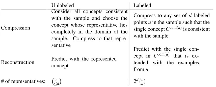
Unlabeled Labeled
Compression
Consider all concepts consistent with the sample and choose the concept whose representative lies completely in the domain of the sample. Compress to that repre-sentative
Compress to any set of d labeled points u in the sample such that the single concept Cdom(u)is consistent with the sample
Reconstruction Predict with the represented concept
Predict with the single con-cept in Cdom(u) that is ex-tended with the examples from u
# of representatives: ≤nd 2d nd
Figure 12: Comparison of the two compression schemes.
A forbidden labeling (Floyd and Warmuth, 1995) of a class C of VC dimension d is a labeled set f of d+1 points in dom(C)that is not consistent with any concept in C. We first note that for a maximum class of VC dimension d there is exactly one forbidden labeling f for each set of d+1 dimensions in dom(C). This is because the restriction C|dom(f) is maximum with dimension d and its size is thus 2d+1−1. Also if C= /0, then VCdim(C) =−1 and the empty set is the only forbidden labeling.
Our Tail Matching Algorithm assigns all concepts in tailx(C) a forbidden labeling of the class
Cx of size(d−1) +1. Since c|r(c)is now a forbidden labeling for Cx, clashes between the tailx(C)
and Cx are avoided. If n is the domain size of C, then the number of such forbidden labelings is
n−1 d
. The class tailx(C)contains the same number of concepts, since C−x=Cx
and Cxand C−x are maximum classes:
|tailx(C)|=|C−x| − |Cx|=
n−1
≤d
−
n−1
≤d−1
=
n−1 d
. (1)
We next show that every tail concept contains some forbidden labeling of Cx and each such forbidden labeling occurs in at least one tail concept. Since any finite maximum class is maximal, adding any concept increases the VC dimension. Adding any concept in tailx(C)−x to Cxincreases
the dimension of Cxto d. Therefore all concepts in tailx(C)contain at least one forbidden labeling of
Cx. Furthermore, since C−x shatters all sets of size d and C−x=Cx∪ (tailx(C)−x), all forbidden
labels of Cx appear in the tail.
We will now show that the Tail Subroutine actually constructs a matching between the forbidden labelings of size d for Cxand the tail concepts that contain them. This matching is unique (Theorem 10 below) and using these matched forbidden labelings as representatives avoids clashes between tail concepts.
We begin by establishing a recursive structure for the tail (see Figure 15 for an example).
Lemma 6 Let C be a maximum class and x6=y be two dimensions in dom(C). If we denote tailx(Cy)
as{ci: i∈I}and tailx(C−y)as{cj: j∈J}(where I∩J= /0),6then there exist bit values{ai: i∈
I},{aj: j∈J}for the y dimension such that tailx(C) ={aici: i∈I}
∪ {ajcj: j∈J}.
Proof First note that the sizes add up as they should (see Equation 1 for the tail size calculation):
|tailx(C)|=
n−1
d
=
n−2 d−1
+
n−2
d
=|tailx(Cy)|+|tailx(C−y)|.
Next we will show that any concept in tailx(Cy) and tailx(C−y) can be mapped to a concept in
tailx(C)by extending it with a suitable y bit. We also have to account for the possibility that there
can be some concepts c∈tailx(Cy)∩tailx(C−y). Concepts in the intersection will need to be
mapped back to two different concepts of tailx(C).
Consider some concept c∈tailx(Cy). Since c∈Cy, both extensions 0c and 1c exist in C. (Note
that the first bit is the y position.) If at least one of the extensions lies in tailx(C), then we can choose
one of the extensions and map c to it. Assume that neither 0c and 1c lie in tailx(C). This means
that these concepts both have x edges to some concepts 0c0,1c0, respectively. But then c0∈Cyand therefore(c,c0)forms an x edge in Cy. Thus c∈/tailx(Cy), which is a contradiction.
Now consider a concept c∈tailx(C−y). It might have one or two y extensions in C. Assume 0c
was an extension outside of the tailx(C). Then this extension has an x edge to some 0c0and therefore
(c,c0)forms an x edge in C−y. It follows that all extensions of c will be in the tail.
Finally, we need to avoid mapping back to the same concept in tailx(C). This can only happen
for concepts in c∈tailx(Cy)∩tailx(C−y). In this case 0c,1c∈C, and by the previous paragraph,
both lie in tailx(C). So we can arbitrarily map c∈tailx(Cy)to 0c and c∈tailx(C−y)to 1c.
The next lemma shows that the order of the restriction and reduction operations is interchange-able (see Figure 16 for an illustration).
6. Note that while Cy⊆C−y, this does not imply that tailx(Cy)⊆tailx(C−y), as the deletion of the concepts(C−y)r
Tail Matching Algorithm
Input: a maximum concept class C Output: a representation mapping r for C
1. If VCdim(C) =0 (i.e., C contains only one concept c), then r(c):= /0. Otherwise, pick any x∈dom(C)and recursively find a representation mapping ˜r for Cx.
2. Expand ˜r to 0Cx∪1Cx:
∀c∈Cx: r(c∪ {x=0}):=˜r(c)and r(c∪ {x=1}):=˜r(c)∪x
3. Extend r to tailx(C)via the subroutine of Figure 14.
Figure 13: The recursive algorithm for constructing an unlabeled compression scheme for maxi-mum classes.
Tail Subroutine
Input: a maximum concept class C, x∈dom(C)
Output: an assignment of representatives to tailx(C)
1. If VCdim(C) =0 (i.e., C={c}=tailx(C)), then r(c):= /0.
If VCdim(C) =|dom(C)|, then tailx(C) =/0and r :=/0.
Otherwise, pick some y∈dom(C), y6=x and recursively find representatives for tailx(Cy)and tailx(C−y).
2. ∀c∈tailx(Cy)rtailx(C−y), find c0∈tailx(C), s.t. c0−y=c, r(c0):=r(c)∪ {y}.
3. ∀c∈tailx(C−y)rtailx(Cy), find c0∈tailx(C), s.t. c0−y=c, r(c0):=r(c).
4. ∀c∈tailx(Cy)∩tailx(C−y), consider the concepts 0c,1c∈tailx(C). Let r1
be the representative for c from tailx(Cy) and r2 be the one from tailx(C−y).
Suppose, wlog, that 0c|r1∪ {y}is a sample not consistent with any concept in Cx.
Then r(0c):=r1∪ {y}, r(1c):=r2.
Figure 14: The Tail Subroutine for finding tail representatives
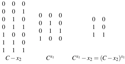
Lemma 7 For any maximum class C and two dimensions x6=y in dom(C), Cx−y= (C−y)x.
Proof We first show that Cx−y⊆(C−y)x. Take any c∈Cx−y. By the definition of restriction,
x1 x3 x4
0 0 0
0 1 0
0 1 1
1 0 0
1 1 0
1 1 1
0 0 1
x1 x3 x4
0 0 0
1 0 0
0 1 0
0 1 1
x1 x2 x3 x4
0 1 0 1 tailx1(C−x2)
0 1 1 0 tailx1(C
x2)
0 1 1 1 tailx1(C
x2)
C−x2 Cx2 tailx1(C)
Figure 15: Illustration of Lemma 6 which shows that tailx1(C)can be composed from tailx1(C
x2)and
tailx1(C−x2); class C is from Figure 2, tails in classes are separated by horizontal lines
and the last column for tailx1(C)indicates whether the concept comes from tailx1(C
x2)
or tailx1(C−x2).
0 0 0
0 0 1
0 1 0
0 1 1
1 0 0
1 1 0
1 1 1
0 0 0
0 1 0
0 1 1
1 0 0
0 0
1 0
1 1
C−x2 Cx1 Cx1−x2= (C−x2)x1
Figure 16: Illustration of Lemma 7 which shows that Cx1−x
2= (C−x2)x1: class C is given in
Figure 2.
follows that 0ayc,1ayc∈C. By first restricting these two concepts in y and then reducing in x we
have 0c,1c∈C−y and c∈(C−y)x, respectively.
Both(C−y)xand Cx−y are maximum classes with the same domain size|dom(C)| −2 and the
same VC dimension. Therefore both have the same size, and since Cx−y⊆(C−y)x, they are in
fact equal.
Corollary 8 Any forbidden labeling of(C−y)xis also a forbidden labeling of Cx.
Proof By the previous lemma, the forbidden labelings of(C−y)x and Cx−y are the same. The
Lemma 9 If we have a forbidden labeling for Cxyof size d−1, then there exists a bit value for the y dimension such that extending this forbidden labeling with this bit results in a forbidden labeling of size d for Cx.
Proof We will establish a bijection between forbidden labelings of Cxof size d that contain y and forbidden labelings of size d−1 for Cxy. Since Cx is a maximum class of VC dimension d−1, it has n−d1forbidden labelings of size d, one for every set of d dimensions from dom(C)rx. Exactly
n−2 d−1
of these forbidden labelings contain y and this is also the total number of forbidden labelings of size d−1 for Cxy.
We map the forbidden labelings of size d for Cx that contain y to labelings of size d−1 by
discarding the y dimension. Assume that a labeling constructed this way is not forbidden in Cxy. Then by extending the concept that contains this labeling with both(y,0)and(y,1)back to Cx, we will hit the original forbidden set, thus forming a contradiction.
It follows that every forbidden set is mapped to a different forbidden labeling and by the count-ing argument above we see that all forbidden sets are covered. Thus the mappcount-ing is a bijection and the inverse of this mapping proves the lemma.
Theorem 10 Let C be any maximum class C of VC dimension d and domain size n. For any x∈ dom(C)we can construct a bipartite graph between the n−d1 concepts in tailx(C) and the n−d1
forbidden labelings of size d for Cxwith an edge between a concept and a forbidden labeling if this labeling is contained in the concept. All such graphs have a unique matching.
Proof The proof is an induction on n=|dom(C)|and d. More precisely, we induct on the pairs
(n,d)(where n≥d) in lexicographic order. The minimal element of this order is(0,0).
Note that in the Tail Matching Algorithm 13 we actually stop when n=d, in which case we have a complete hypercube with no tail and the matching is empty. Also for d=0, there is a single concept which is always in the tail and gets matched to the empty set.
Inductive hypothesis: For any maximum classC, such thate (|dom(Ce|,VCdim(Ce))<(n,d)the statement of the theorem holds.
Inductive step. Let x,y∈dom(C) and x6=y. By Lemma 6, we can compose tailx(C) from
tailx(Cy)and tailx(C−y). Since VCdim(Cx) =d−1 and|dom(C−x)|=n−1,7then(n−1,d),(n−
1,d−1)<(n,d) and we can use the inductive hypothesis for these classes and assume that the desired matchings already exist for tailx(Cy)and tailx(C−y).
Now we need to combine these matchings to form a matching for tailx(C). See Figure 14 for a
description of this process. Concepts in tailx(C−y)are matched to forbidden labelings of(C−y)x
of size d. By Lemma 8, any forbidden labeling of(C−y)xis also a forbidden labeling of Cx. Thus
this part of the matching transfers to the appropriate part of tailx(C) without alterations. On the
other hand, tailx(Cy) is matched to labelings of size d−1. We can make them labelings of size
d by adding some value for the y coordinate. Some care must be taken here. Lemma 9 tells us that one of the two extensions will in fact have a forbidden labeling of size d (that includes the y coordinate). In the case where just one of two possible extensions of a concept in tailx(Cy)is in the
tailx(C), there are no problems: the single concept will be the concept of Lemma 9, since the other
concept lies in Cx and thus does not contain any forbidden labelings. There is also the possibility
that both extensions are in tailx(C). From the proof of Lemma 6 we see that this only happens to the
concepts that are in tailx(Cy)∩tailx(C−y). Then, by Lemma 9, we can figure out which extension
corresponds to the forbidden labeling involving y and use that for the tailx(Cy)matching. The other
extension will correspond to the tailx(C−y)matching. Essentially, where before Lemma 6 told us
to map the intersection tailx(Cy)∩tailx(C−y)back to tailx(C)by assigning a bit arbitrarily, we now
choose a bit in a specific way.
So far we have shown that the matching exists. We still need to verify its uniqueness. From any matching for tailx(C)we will show how to construct matchings for tailx(C−y)and tailx(Cy)with
the property that two different matchings for tailx(C)will disagree with the constructed matchings
for either tailx(C−y)or tailx(Cy). Now, uniqueness follows by induction.
Consider any concept c in tailx(C), such that c−y∈tailx(Cy)rtailx(C−y). Then c−y lies
in C−y, but not in tailx(C−y). Therefore c−y must belong to either 0(C−y)x or 1(C−y)x,
which means that this concept cannot contain a forbidden set for (C−y)x. We claim that any
forbidden set of c for Cx must contain y. Otherwise such a set would be forbidden for Cx−y, which by Lemma 7 equals(C−y)x. By a similar argument, concepts c∈tail
x(C), such that c−y∈
tailx(C−y)rtailx(Cy)have to be matched to forbidden sets that do not contain y (since a forbidden
set of size d for Cxthat contains y, becomes a forbidden set of size d−1 for Cxyjust by removing y, and condition c−y∈/tailx(Cy)implies that c does not contain any such forbidden sets).
From these two facts it follows that if a concept in tailx(C)is matched to a forbidden set
contain-ing y, then c−y∈tailx(Cy), and if it is matched to a set not containing y, then c−y∈tailx(C−y).
We conclude that a matching for tailx(C)splits into a matching for tailx(C−y)and a matching for
tailx(Cy). This implies that if there are two matchings for all of tailx(C), then there are either two
matchings for tailx(C−y)or two matchings for tailx(Cy).
Theorem 11 The Tail Matching Algorithm of Figure 13 returns a representation mapping that sat-isfies both conditions of the Main Definition.
Proof Proof by induction on d=VCdim(C). The base case is d=0: this class has only one concept which is represented by the empty set.
The algorithm recurses on Cxand VCdim(Cx) =d−1. Thus we can assume that it has a correct representation mapping for Cxthat uses sets of size at most d−1 for the representatives.
Bijection condition: The representation mapping for C is composed of a bijection between 1Cx and all sets of size≤d containing x, a bijection between 0Cx and all sets of size<d that do not contain x, and finally a bijection between tailx(C)sets of size equal d that do not contain x.
No clashes condition: By the inductive assumption there cannot be any clashes internally within each of the subclasses 0Cx and 1Cx, respectively. Clashes between 0Cx and 1Cx cannot occur be-cause such concepts are always differentiated on the x bit and x belongs to all representatives of 1Cx. By Theorem 10, we know that concepts in the tail are assigned to representatives that define a forbidden labeling for Cx. Therefore, clashes between tail
x(C)and 0Cx, 1Cx are avoided. Finally,
we need to argue that there cannot be any clashes internally within the tail. By Theorem 10, the matching between concepts in tailx(C)and forbidden labeling of Cx is unique. So if this matching
resulted in a clash, that is, c1|r1∪r2=c2|r1∪r2, then both c1and c2would contain the forbidden
labelings specified by representative r1and r2. By swapping the assignment of forbidden labels
thus contradicting the uniqueness of the matching.
Note that by Corollary 4, the unlabeled compression scheme produced by our recursive algorithm induces a d-orientation of the one-inclusion graph: orient each edge away from the concept that contains the dimension of the edge in its representative. As was the case for the orientation pro-duced by the Min-Peeling Algorithm, the resulting orientation is acyclic. As a matter of fact a topological order can be constructed by ordering the concepts of C as follows: 0Cx,1Cx,tailx(C).
The concept within tailx(C) can be ordered arbitrarily and the concepts within 0Cx and 1Cx are
ordered recursively based on the topological order for Cx.
7. Miscellaneous Lemmas
We conclude with some miscellaneous lemmas that highlight the combinatorics underlying the un-labeled compression schemes for maximum classes. The first one shows that the representatives constructed by our Tail Matching Algorithm induce a nesting of maximum classes. This is a special property, because there are cases where the simpler Min-Peeling Algorithm produces a representa-tion mapping that does not have this property (not shown).
Lemma 12 Let C be a maximum concept class with VC dimension d and let r be a representation mapping for C produced by the Tail Matching Algorithm. For 0≤k≤d, let Ck={c∈C s. t. |r(c)| ≤
k}. Then Ck is a maximum concept class of VC dimension k.
Proof Proof by induction on d. Base case d=0: the class has only one concept and the lemma clearly holds.
The lemma trivially holds for k=0 or k=d. Otherwise let x∈dom(C)be the first dimension used in the recursion of the Tail Matching Algorithm and assume by induction that the lemma holds for Cx. Consider which concepts in C belong to Ck. Clearly none of the concepts in tailx(C)lie in
Ck because their representatives are of size d>k. From the recursion of the algorithm it follows
that Ck=0Cxk∪1Ckx−1, that is, it consists of all concepts in 0Cx with representatives of size≤k in
the mapping for Cx, plus all the concepts in 1Cxwith representatives of size≤k−1 in the mapping for Cx. By the inductive assumption, Ckx and Cxk−1 are maximum classes with VC dimension k and k−1, respectively. Furthermore, the definition of Ckimplies that Ckx−1⊂Ckx.
Since |Ck|=|0Cxk|+|1Ckx−1|= n≤−k1
+ ≤nk−−11 = ≤nk, the class Ck has the right size and
VCdim(Ck)≥k. We still need to show that Ck does not shatter any set of size k+1. Consider any
such set that does not contain x. This set would have to be shattered by Ck−x=Ckx∪Ckx−1=Ckx,
which is impossible. Now consider any set A of size k+1 that does contain x. All the 1 values for the x coordinate happen in the 1Ckx−1 part of Ck. Thus Arx must be shattered by Cxk−1 whose VC
dimension is again one too low.
We actually proved that the Ck produced by the representation mapping of the Tail Matching
Al-gorithm always satisfy the recurrence Ck=0Ckx∪1Ckx−1. On the other hand there are nestings of
maximum concept classes C0⊂C1⊂. . .⊂Cd =C, where Ck has VC dimension k, for which the
above recurrence does not hold (not shown).
Open Problem 1. We do not know whether for any nesting C0⊂C1⊂. . .⊂Cd=C of maximum
classes, where Ck has VC dimension k, there always exists a representation mapping that induces