Prioritization Methods for Accelerating MDP Solvers
David Wingate [email protected]
Kevin D. Seppi [email protected]
Computer Science Department Brigham Young University Provo, UT 84602, USA
Editor: Sridhar Mahadevan
Abstract
The performance of value and policy iteration can be dramatically improved by eliminating redun-dant or useless backups, and by backing up states in the right order. We study several methods designed to accelerate these iterative solvers, including prioritization, partitioning, and variable reordering. We generate a family of algorithms by combining several of the methods discussed, and present extensive empirical evidence demonstrating that performance can improve by several orders of magnitude for many problems, while preserving accuracy and convergence guarantees.
Keywords: Markov Decision Processes, value iteration, policy iteration, prioritized sweeping, dynamic programming
1. Introduction
This paper systematically explores the idea of minimizing the computational effort needed to com-pute the optimal policy (with its value function) of a discrete, stationary Markov Decision Process using an iterative solver such as value or policy iteration. The theme of our exploration can be stated generally as “backing up states in the right order,” and to accomplish that, we present and discuss several methods of differing complexity which structure value dependency and prioritize compu-tation to follow those dependencies. We have named the resulting family of algorithms General
Prioritized Solvers, or GPS.
between policy improvement steps. In addition, GPS can enhance algorithms that propagate dif-ferent forms of information (not just value information). For example, Munos and Moore (2002) propagate both “influence” and “variance” throughout a problem using a form of value iteration. In this more abstract sense, the principle of propagating knowledge throughout a space as quickly and efficiently as possible is applicable to almost all systems.
Two principal observations motivated this work. First, many backups performed by value it-eration can be useless. Value itit-eration is almost a pessimal algorithm, in the sense that it never leverages any advantage a sparse transition matrix (and/or sparse reward function) may offer: it always iterates over and updates every state, even if such a backup does not (or cannot) change the value function. An intuitive improvement is this: if, on the previous sweep, only a handful of states changed value, why back up the value of every state on the next sweep? The only useful backups will be to those states which depend upon states that changed on the previous sweep. Similar obser-vations about the efficient ordering of work can be made about policy iteration: it is best to wait to compute the policy of a state s until a good policy for the dependents of s has been determined.
Second, almost all backups are naively ordered. For example, ordering the states in an acyclic problem such that the rows in the transition matrix are triangular (corresponding to a topological
sort) yields a O(n)solution; but solving the same system in an arbitrary order yields an expected
O(n2)solution time. Additionally, as information backpropagates through a value function estimate,
the optimal ordering may change. Dynamically generating a good backup ordering in an efficient way is one of the central issues we examine.
The idea of efficient computation applied to value iteration and policy iteration is not new, but it has not received a dedicated treatment. This paper makes a fourfold contribution: first, it studies pri-oritization metrics systematically, comparing and contrasting them to each other. Most other papers have only presented a metric in isolation, as a heuristic performance enhancer. Prioritized Sweeping (Moore and Atkeson, 1993), for instance, uses Bellman error as a priority metric, but we demon-strate that another equally simple metric can perform better. Second, this paper points out how the complexity introduced with the priority metrics can be managed through the use of partitioning, which is an issue other researchers have not addressed. Partitioning also enables prioritized policy iteration, which has not been studied previously. Third, this paper introduces a new priority metric,
H2, and an effective variable reordering algorithm designed to improve performance. Both are
stud-ied empirically, and some general guidelines for their use are established. Fourth, and somewhat in contrast to most asynchronous value iteration proofs of convergence (such as Bertsekas, 1982, 1983; Gullapalli and Barto, 1994), we point out that not every state needs to be backed up during each sweep in order to guarantee convergence. In fact, some states may never need to be backed up at all, which is valuable for optimizing performance.
2. The GPS Family of Algorithms
There are three principal enhancements we use to accelerate value and policy iteration: prioritiza-tion, partitioning and variable reordering. Sections 2.1, 2.3 and 2.5 discuss each in detail, along with issues that each raises. A general discussion of convergence, stopping, and complexity is deferred until Section 2.6. We shall study many combinations of these enhancements, but consider all vari-ants to be members of a single family. We begin with a prototype MDP solver, which has elements common to all members:
Algorithm 1 Abstract GPS
Initialization
1: // Partition the problem
2: // Order variables within each partition
3: // Compute initial partition priorities
Main Loop
1: repeat
2: // Select a partition p
3: // Compute the optimal policy and value function of states in p,
// keeping all other partitions constant
4: // Recompute priorities of partitions depending on p
5: until convergence
To simplify the following discussions, all of the MDPs we consider are discounted, infinite horizon, stationary and positive bounded (all rewards are positive and finite).
2.1 Prioritization
The first method we use to improve efficiency is the prioritization of backups. Instead of naively sweeping over the entire problem, we wish to work our way backwards through the problem: we correct the value function estimate (and policy) for a state s by backing it up, and then correct the value function estimate (and policy) for all states which depend upon s. This has the effect of focusing computation in regions of the problem which are expected to be maximally productive, and simultaneously avoids useless backups.
To accomplish this, we begin with a standard value function definition:
V(s) =max
a∈A
(
R(s,a) +γ
∑
s0∈S
Pr(s0|s,a)V(s0) )
. (1)
Here, s∈S is a state, a∈A is an action,γ∈[0,1)is the discount factor, R(s,a)is the reward function,
and Pr(s0|s,a)is the probability of transitioning to state s0if action a is taken in state s. Algorithm
2 shows the traditional value iteration algorithm, without prioritization.
We use Bellman error to characterize how useful any given backup is, and then construct differ-ent metrics based on the Bellman error as the priority in a priority queue:
Bt(s) =max a∈A
(
R(s,a) +γ
∑
s0∈S
Pr(s0|s,a)Vt(s0)
)
Algorithm 2 Standard Value Iteration
1: V0←0
2: repeat
3: for all s∈S do
4: Vt(s)←maxa∈A{R(s,a) +γ∑s0∈SPr(s0|s,a)Vt−1(s0)}
5: end for
6: t←t+1
7: until convergence
Note that this should not be considered a one-step temporal difference: Bellman error represents the amount of potential change to the value function, assuming that a certain state was backed up, as opposed to the actual difference between two value function estimates separated by one timestep. Peng and Williams (1993) called this value the prediction difference. We will let
Mt =kBtk∞
be the largest potential update in the system, wherek · k∞ represents max-norm. This quantity is
commonly called the Bellman error magnitude (Williams and Baird, 1993).
We build different prioritization metrics upon the Bellman error function. The first metric we will analyze, H1, is equal to the Bellman error itself:
H1t(s) =Bt(s).
The second metric is:
H2t(s) =
Bt(s) +Vt(s) if Bt(s)>ε
0 otherwise.
When it is not important which prioritization metric is used, we will use Ht(s)to refer to a generic
one. The next section discusses the semantics of each metric.
Once a state s is backed up, the priority of any state depending on s must be recomputed. The
state dependents of a state is the set of all states who have some probability of transitioning to s,
and therefore whose value depend on the value of s. We define it as
SDS(s) =
s0:∃aPr(s0|s,a)6=0 .
Algorithm 3 shows a prioritized version of value iteration.
As noted, we only consider positive bounded MDPs. Creating a positive bounded MDP can be accomplished by adding a constant C to the reward function; since we will initialize the value
function estimate to 0, this ensures that Vt≤V∗(where V∗is the value of the optimal policyπ∗). This
does not change the resulting policy, and, as Zhang et al. (1999) point out, “the value function of
the original [MDP] equals that of the transformed [MDP] minus C/(1−γ), where C is the constant
Algorithm 3 Prioritized Value Iteration
1: repeat
2: s←arg maxξ∈SH(ξ)
3: V(s)←maxa∈A{R(s,a) +γ∑s0∈SPr(s0|s,a)V(s0)}
4: for all s0∈SDS(s)do
5: // recompute H(s0)
6: end for
7: until convergence
2.2 Selecting Metrics
The H1 prioritization metric is the most obvious metric, and has been studied before (although not in contrast to other metrics, and in somewhat different contexts than ours). Using it, GPS can be thought of as a greedy reduction in the error of the value function estimate. This has the tendency to propagate information quickly throughout the state space, but it also tends to leave large regions only partially converged, and therefore does not necessarily propagate correct information quickly. The H2 metric has a very different effect on computation order. The intuition is this: if there is a
value that is more thanεaway from its optimal value, the value will eventually need to be corrected.
Since large values (generated from large rewards, or small loops) have greater influence on the value function than small values, H2 converges large values before propagating their influence throughout the state space. This tends to ensure that regions are fully converged before anything depending on the region is processed. Experimental results illustrating these effects are shown in Figure 1.
The results in Section 4 demonstrate that neither H1, H2, nor standard value iteration induce an optimal backup ordering for all MDPs. However, each performs better than the others for some problems. The question of which metric should be used on a new problem naturally arises, but it is difficult to find topological features which accurately predict the performance of each metric. Often, the best metric seems to be a hybrid of all three.
Normal value iteration yields a very good backup order when a problem is close to being fully connected (and thus, whenever states are highly interdependent). The obvious corollary is that value iteration is also very good for any subgraph that is close to fully connected. Value iteration performs poorly when the problem exhibits highly sequential (and thus, asymmetric) dependencies, which can be due to a large number of strongly connected components, or a large graph diameter relative to the number of nodes.
The H1 metric performs best in graphs which have highly sequential dependencies, which occur in acyclic graphs and in graphs with long loops. The H1 metric excels at avoiding useless backups, but tends not to iron out feedback loops completely, meaning that states within such loops must often be processed multiple times.
Figure 1: Images of partially converged value functions for the SAP problem (described in Section 3). The left function was generated with H1, and the right function was generated with
H2. For both images, the x axis represents position, the y axis represents velocity, and
the z axis represents the value of the state. Notice the “stair step” in the left image near the primary reward (the peak in the middle of the space). This will eventually need to be corrected, and the change will propagate throughout the entire problem, resulting in extra computation. In addition, notice the many imperfections; each of them will eventually need to be corrected. The right function is much cleaner, because H2 tends to drive regions of the problem to convergence before moving on. Green (light gray) and red (medium gray) are different controls; a dark blue color (dark gray) indicates that a state has never been processed. Both images are frames from a video which is available in the on-line appendix.
A B C D
0 0.5 1 1.5 2 2.5
0 20 40 60 80 100
Summed value function estimate
Number of backups
Value iteration Partitioned VI with H1 metric Partitioned VI with H2 metric
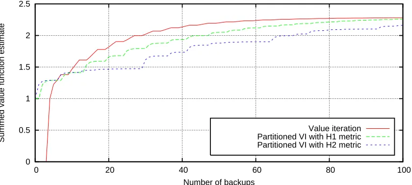
Figure 3: Performance of two GPS variants on the problem in Figure 2, using one state per par-tition and a value iteration subsolver (see Figure 6 for an explanation of the different
algorithms). Shown is∑s∈SV(s)versus the number of backups. Reaching a higher sum
in fewer backups is better.
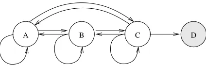
states in a round-robin fashion, which is nearly optimal (it is not fully optimal because it repeatedly backs up state D, even though it does not need to do so).
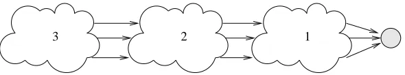
H2 performs best in a hybrid setting, which we illustrate using Figure 4. Each cloud represents
a cluster of highly interdependent states (perhaps even strongly connected components); clusters are weakly connected to each other. The values of states within each cluster should be converged before moving on to process the next cluster, but within each cluster, standard value iteration should be employed. By themselves, each metric performs poorly: value iteration performs useless backups by working on clusters two and three before information has propagated back to them; H1 has the tendency to prematurely move on to the second and third clusters before the first cluster has converged, and H2 correctly prioritizes clusters, but functions poorly within each cluster.
A good algorithm should select a cluster and work on it until convergence, then move on to the next cluster. This is exactly the way that GPS functions, except that it also employs partitions (as discussed in the next section). Either H1 or H2 serves as a guide between partitions, but within each partition, round-robin updating occurs.
2.3 Partitioning
Although prioritization reduces the total number of backups performed, the overhead of managing
the priority queue can be prohibitively high. Each state s (and each s0∈SDS(s)) must be extracted,
reprioritized, and reinserted into the queue, resulting in several O(log n) operations per backup
3 2 1
Figure 4: An example illustrating when hybrid metrics are close to optimal. Clouds represent clus-ters of highly interdependent states; arrows represent some of the arcs in the transition matrix. Variants of GPS perform very well on problems of this sort if partitions corre-spond to clusters.
Two observations direct our solution: first, we can accept some backups that do not occur in strict priority order. Second, any single state (typically) depends on multiple other states; it would be ideal to postpone the reprioritization of a state until multiple dependencies have been backed up. A good principle is to group states together into sets, and to work on the sets, instead of individual states. This accomplishes both goals: it efficiently approximates the backup order induced by the priority metric, and it tends to ensure that multiple dependencies are resolved before moving on. The specific partitioning used therefore navigates the trade-off between useless backups (there might be states in the partition that did not need to be processed) and priority queue overhead (it is faster to update them anyway, because it takes too long to determine which ones are useless). Additionally, with partitioning in place, a prioritized version of policy iteration may be created, as described in the next section.
Our partitioned, prioritized algorithm selects a high-priority partition p, solves the states in the partition, and then reprioritizes any partition which depends upon anything in p. Thus, running GPS with a single partition containing all states is equivalent to normal value/policy iteration, while running it with a single state per partition generates backups in strict priority order (this is actually not always the case, as explained in the next section).
We use the following definitions to describe a partitioned, prioritized algorithm. Let each p∈P
be a partition, which is a set of states. We define the state dependents of a partition to be the set of all states whose value depends on some state in the partition p:
SDP(p) =[ s∈p
SDS(s).
Let Psbe a function mapping states to their partitions. We define the partition dependents of a state
to be the set of partitions which contain a state whose value depends on s:
PDS(s) = [ s0∈SDS(s)
Ps(s0).
We define the partition dependents of a partition to be the set of all partitions that contain at least one state that depends on the value of at least one state in p:
PDP(p) =[ s∈p
PDS(s).
We define the priority between two partitions as
HPPt(p,p0) = max
Note that in general, HPPt(p,p0)=6 HPPt(p0,p). We define the priority of a partition as
HPt(p) =max
p0 HPPt(p,p
0).
Algorithm 4 shows a general partitioned, prioritized solver.
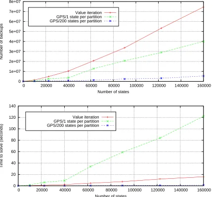
As shown in Figure 5, adding more states to the partitions dramatically improves performance. Both variants of GPS perform fewer backups to the value function than normal value iteration, but because the variant with 200 states per partition eliminates priority queue overhead, the time needed for it to reach a solution drops by two orders of magnitude. Counter-intuitively, it even performed fewer backups than the variant which used only one state per partition. This indicates that the intra-partition backup order is better than the order imposed by the priority metric.
Figure 3 demonstrates one situation in which using priority metrics with partitioning can be suboptimal, and that it is not always desirable to solve partitions exactly. In this example, the best solver is normal value iteration, which can be thought of as an algorithm which solves each partition inexactly. That is, it performs exactly one backup within each partition, and then moves on to the next partition, in a round-robin fashion. Both of the other algorithms attempt to solve each
partition to withinεof optimal; because they back up the states in the partition multiple times, the
value function of the states slowly spirals upwards. Once they are withinεof their optimal value,
the solvers select another partition. This example suggests that that partitioned solvers will be suboptimal whenever partitions are highly intra-dependent and highly inter-dependent. Of course, the example also illustrates the fact that the prioritization metrics (either at the state level, or the partition level) are only an approximation of the optimal backup ordering.
There are many possible ways to generate good partitions. If states have geometrical information associated with them, it can be used to generate partitions containing states that are near to each other. If not, more general k-way graph partitioning algorithms, such as multilevel coarsening or recursive spectral bisection, may be used (see Alpert, 1996, for an excellent dissertation on the subject). k-way graph partitioners generate partitions that minimize the cumulative weight of cross-partition edges, which is desirable because it tends to ensure that highly interdependent states are in the same partition. Automatic, variable resolution partitioners could be used, such as those described by Moore and Atkeson (1995) or Munos and Moore (2002). It may also be possible that techniques from state aggregation literature may help. Dean and Givan (1997) describe a “stable cluster” creation technique, for instance, with properties that are desirable for a partition.
Combining partitioning with prioritization is useful for other reasons, which are not explored in this work. Partitioning is a good domain decomposition, which enables an efficient, naturally parallelizable algorithm (Wingate and Seppi, 2004b). In addition, the H2 metric (combined with partitioning) exhibits excellent disk-based-cache behavior, which is desirable when attempting to solve problems so large they cannot fit into available RAM (Wingate and Seppi, 2004a).
Our experiments tested both geometrically generated partitions as well as partitions generated by the METIS package (see, for example, Karypis and Kumar, 1998). Section 4 presents results exploring different edge cut criteria.
2.4 Solving a Partition
0 1e+07 2e+07 3e+07 4e+07 5e+07 6e+07 7e+07 8e+07
0 20000 40000 60000 80000 100000 120000 140000 160000
Number of backups
Number of states Value iteration
GPS/1 state per partition GPS/200 states per partition
0 20 40 60 80 100 120 140
0 20000 40000 60000 80000 100000 120000 140000 160000
Time to solve (seconds)
Number of states Value iteration
GPS/1 state per partition GPS/200 states per partition
Algorithm 4 Prioritized, Partitioned Value and Policy Iteration
Initialization
1: for all s∈S do
2: V0(s)←0
3: H0(s)←maxa∈AR(s,a)
4: end for
5: for all p∈P do
6: HP0(p)←maxs∈p,a∈AR(s,a)
7: for all p0∈P do
8: HPP0(p,p0)←0
9: end for 10: end for
11: p←arg maxξ∈PHP0(ξ)
12: t←1
Main loop
1: repeat
2: // compute the optimal policy and value function of states in p
3: solve(p)
4:
5: // update partition priority for all dependent partitions
6: for all p0∈PDP(p)do 7: HPPt(p0,p)←0
8: hmax←0
9: for all s0∈p0∩SDP(p)do
10: // recompute Ht(s0)
11: hmax←max(hmax,Ht(s0))
12: end for
13: HPPt(p0,p)←hmax
14: HPt(p0)←maxξHPPt(p0,ξ)
15: end for
16: p←arg maxξ∈PHPt(ξ)
17: t←t+1
be used. It is even possible to use a partitioned, prioritized solver (indeed, such an idea could be extended to more than two levels), although hierarchical partitioning is not explored in this work.
We require that the value of the states in the partition be computed accurately (that is, to withinε
of exact) because the value function may be needed in the context of a larger algorithm, but more importantly because both priority metrics depend upon accurate value function estimates. In other words, if we use policy iteration as a solver, and use an iterative policy evaluation method, we cannot stop when just the policy has converged; rather, we must wait until the value function has converged as well.
It is clear how to use value iteration to solve p, but it is less clear how to use policy iteration. Policy improvement is easy, but how do we evaluate the value of the states in p? Recall that policy
evaluation is the process of computing the value function for a single policyπ. This eliminates the
max operator in Eq. 1, simplifying it to V(s) =R(s,π(s)) +γ∑s0∈SPr(s0|s,a)V(s0). This is a linear
system of|S|equations in |S|unknowns; in matrix-vector notation, it is equivalently expressed as
v=rπ+γPπv, where P is the transition probability matrix of policyπand rπis the reward under
policy π. Note that this has the same form as the more general problem x=Ax+b, which is
equivalent to(I−A)x=b.
The key observation is the fact that if the value and policy of states outside the partition are held constant, their values may be temporarily “folded” into the right-hand side vector, and a new
sub-problem created. As an example, consider the general problem Ax=b, where A is a 2x2 matrix.
Suppose that we wish to solve only for variable 0 while holding variable 1 constant. We may expand this system (indexing with array notation) as
A[0,0]x[0] +A[0,1]x[1] = b[0]
A[1,0]x[0] +A[1,1]x[1] = b[1]
and, since x[1]is constant, rewrite it as
A[0,0]x[0] =b[0]−A[0,1]x[1] =b0[0]
A[1,0]x[0] =b[1]−A[1,1]x[1] =b0[1],
where b0is the new vector that results from the folding operation. This yields a set of two equations
with one unknown. Either may be used to solve for variable 0.
More generally, assume that we are given an n×n matrix A and a partition p which contains a
set of variable indices that we wish to solve for. The equation for variable i is
n
∑
j=0A[i,j]x[j] = b[i]
∑
j∈pA[i,j]x[j] +
∑
j6∈p
A[i,j]x[j] = b[i]
∑
j∈pA[i,j]x[j] = b[i]−
∑
j6∈pA[i,j]x[j]
∑
j∈pA[i,j]x[j] = b0[i].
This yields n equations in|p|unknowns, which is an over-constrained system. We wish to select a
corresponding to the variable indices in the partition. Specifically, we may define a diagonal selector
matrix as
Kp[i,i] =
1 i∈p
0 otherwise.
Then, to select a subset of equations from A,x and b, we will let A0=KpAKp, x0=Kpx, and b0=Kpb.
Note that A0is still an n×n matrix, but with many empty rows and columns. If row i in A0is empty,
column i will also be empty, and the corresponding entries in both both x0and b0will also be zero.
The entire system may be compacted by eliminating such zero entries and mapping variable indices from the original system to new variable indices in a compacted system, which may then be passed to an arbitrary subsolver. Selection and compaction can be accomplished simultaneously through the use of prolongation and restriction operators (Saad, 1996), but we have adopted the current approach for simplicity of explanation. We note that GPS with this fold/extract method can be considered a prioritized Multiplicative Schwarz Procedure (Schwarz, 1890; Saad, 1996).
Once the problem A0x0=b0is constructed, any number of direct or indirect linear system solvers
can be used. Exact policy evaluation usually involves inverting a matrix, which is typically a O(n3)
operation. Since we only need to solve A0x0=b0 to withinε, and because of our interest in
per-formance, we we can opt instead for approximate policy evaluation. Fortunately, this does not compromise the accuracy of the final solution: Bertsekas and Tsitsiklis (1996) establish the funda-mental soundness of approximate policy evaluation, and provides bounds on the optimality of the final policy based on the evaluation error.
In this work, we use Richardson iteration (which is equivalent to value iteration) and GMRES as policy evaluators. GMRES is considered by the numerical analysis community to be the standard it-erative method for large, sparse, asymmetric matrices. Saad (1996) presents an excellent discussion of iterative methods and Barrett et al. (1994) present template-based implementations of common iterative methods.
2.5 Variable Reordering
As noted previously, it is possible to use standard value iteration to solve a partition. We would like to optimize this step in the algorithm, but we have already seen that we cannot use a priority queue – the overhead is excessive, which is why we used partitions in the first place. Instead of a good dynamic ordering, we therefore opt for a good static ordering. Specifically, we wish to reorder the states in the partition such that for each sweep, they are backed up in an approximately optimal order. This ordering of states is computed once, during initialization. Note that variable reordering is only effective when Gauss-Seidel iterations are used; it does not affect Jacobi-style iterations, and may not affect other methods of solving linear systems. In particular, variable reordering is only applicable to prioritized policy iteration if partitions are evaluated using a Gauss-Seidel iterative method.
Algorithm 5 Variable reordering
1: // Initialization:dcis an array representing the in-degree of each state
2: dc←0
3: for all s∈p do
4: for all a∈A do
5: for all s0∈p do if((Pr(s0|s,a)6=0)thenincrement(dc[s0])
6: end for
7: end for 8:
9: // Main loop:finalorderis an array representing the final state ordering
10: for i=0..|p| −1 do
11: let s be the index of the smallest non-negative value indc
12: dc[s]← −1
13: finalorder[|p| −1−i]←s
14: for all a∈A do
15: for all s0∈p do if((Pr(s0|s,a)6=0)thendecrement(dc[s0])
16: end for 17: end for
The reason for this follows. We begin with the generic problem x=Ax+b, where A is a matrix
and x,b are column vectors. This suggests an iterative method of the form
xt+1=Axt+b (2)
which corresponds to a Jacobi-style iterative method. Now, let A= (L+D+U), where L is the
lower-triangular part of A, D is the diagonal part, and U is the upper-triangular part. Using
Gauss-Seidel iterations, Eq. 2 can be expressed as xt+1=Lxt+1+ (U+D)xt+b (recall that Gauss-Seidel
iterations use state values as soon as they are available). This can be rearranged to yield
xt+1= (I−L)−1(U+D)xt+ (I+L)−1b. (3)
This is the most basic regular splitting of the matrix A; see Puterman (1994) for a more comprehen-sive treatment of regular splittings and of the specifics of Gauss-Seidel vs. Jacobi iterations.
It is well known that both asynchronous and synchronous relaxations of the form xt+1= f(xt)
converge when f satisfies the definitions of a contraction mapping (Bertsekas and Tsitsiklis, 1989). Proofs of contraction have been constructed for several important cases, including linear relaxations.
Iterations in the form of Eq. 2 are guaranteed to converge if the spectral radiusρ(A)<1.
The convergence of Eq. 3 is therefore governed by ρ((I−L)−1(U+D)), which is a difficult
expression to simplify. However, it is also well known thatρ(AB)<kAkkBkfor any matrix norm;
since the infinity-norm of a matrix corresponds to the largest row-sum in the matrix, convergence
will be governed byk(I−L)−1k∞andk(U+D)k∞. (Tangentially, we note that, because(I−L)is
lower-triangular, its inverse is also lower-triangular, and the eigenvalues therefore correspond to the diagonal entries. It is easy to show that the diagonals will still be ones after inverting, meaning that
ρ((I−L)−1)is simply 1). We therefore seek some permutation of A which will minimize either
a minimizing permutation is obtained, and the graph defined by the matrix is acyclic, (U+D) is empty, and the system converges in one pass.
As Knuth (1993) states, this problem is NP-complete, because it includes as a very special case the “Feedback Arc Set” problem, which “was shown to be NP-complete in Karp’s classic paper (Miller and Thatcher, 1972)”. However, heuristics have been proposed: Knuth (1993) experiments with a downhill method to find a permutation that is locally optimal (in the sense that moving any individual row increases the row-sum), but his method is computationally expensive. Modified topological sorts (in which any edge that completes a cycle is deleted) have also been proposed which are efficient, and which form the basis of the strategy we follow.
The foregoing analysis has been in terms of a generic matrix A. However, the transition matrix of a discrete MDP depends on the operative policy at any given time. What matrix should be used to compute a new variable ordering? We use an aggregate matrix which incorporates all of the transitions possible under any policy, all of which are weighted equally. This represents an implicit assumption that we are optimizing for an expected case where all policies are equally likely, but if additional information about the likelihood of different policies is available, it could be leveraged during this phase.
The final variable reordering algorithm is a modified topological sort, and is shown in Algorithm
5. The algorithm operates on a partition p, and generates the arrayfinalorder, which lists the order
in which states should be backed up.
2.6 Convergence, Stopping Criteria and Complexity
Convergence of GPS with a value-iteration subsolver is established by noting that it is an asyn-chronous variant of traditional value iteration. Convergence is guaranteed for such algorithms pro-vided that every state is backed up infinitely often (Bertsekas, 1982, 1983; Gullapalli and Barto, 1994). Practically, this can be guaranteed as long as no state is starved of backups. In our algo-rithm, states will be backed up until they have converged, at which point a new set of states will be
selected. If a state has some Bt(s)>ε, it will eventually be backed up; if no such state exists, the
problem is solved. Convergence of approximate policy iteration and asynchronous policy iteration has been established by Bertsekas and Tsitsiklis (1996); once again, the stipulation is that each state must be visited infinitely often, and once again, it is clear that our algorithm does not starve any
state that has Bt(s)>ε.
Here, we also note that if a state s never has Bt(s)>ε, it never needs to be backed up. Of course,
there is no performance gain in detecting that a single state never needs to be backed up, because
it takes just as long to compute Bt(s) as it does to back the state up – but partitions change that.
Because the states in a partition p are “blocked off” from the rest of the problem, detection of the
fact that they may not need to be backed up can be highly efficient: only Bt of the cross-partition
dependencies must be examined. If they never move above ε, nothing in p needs to be backed
up (assuming the partition is internally solved). Thus, the “infinite updates” stipulation of most asynchronous convergence proofs represent sufficient conditions, but not necessary conditions.
Stopping criteria are easily established. The largest difference between a value function estimate and the optimal value function can be characterized in terms of the Bellman error magnitude. This has already been accomplished by Williams and Baird (1993); similar results can be easily derived by using equation 6.3.7 of Puterman’s book (Puterman, 1994):
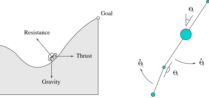
Name Description
PI-Rich Policy iteration with Richardson policy evaluator
PI-GMRES Policy iteration with GMRES policy evaluator
PPI-Rich-H1 Partitioned PI, prioritized w/H1, using Richardson evaluator
PPI-Rich-H2 Same, but with H2 priority metric
PPI-GMRES-H1 Partitioned PI, prioritized w/H1, using GMRES evaluator
PPI-GMRES-H2 Same, but with H2 priority metric
VI Standard value iteration
VI-VRE Value iteration with partitions, NO priority, and variable reordering
PVI-H1 Partitioned value iteration, prioritized with H1
PVI-H1-VRE Same, plus variable reordering
PVI-H2 Partitioned value iteration, prioritized with H2
PVI-H2-VRE Same, plus variable reordering
Figure 6: Algorithms tested.
The maximum difference provides a natural stopping criterion. The algorithm can stop when Mt<
ε(1−γ), and will be guaranteed to have anε-optimal policy. A more common bound (for example,
Puterman, 1994) is that ifkVt+1−Vtk<ε(1−γ)/2γ, thenkVt+1−V∗k<ε/2. The slight difference
in the two equations can be accounted for by noting that we previously stipulated that all rewards be positive (which allows us to provide a tighter bound by avoiding absolute values), and because of a minor difference in time subscripting.
The space complexity of GPS is quite good. The largest overhead comes from the need to store a partial inverse model, but this is always a subset of the whole problem. Additional memory is
needed for the priority queue (O(|P|)), for the state-to-partition mapping (O(|S|)), and the
partition-to-state maps (O(|P|+|S|)).
3. Experimental Setup
We tested twelve different combinations of the basic enhancements we have discussed, which are shown in Figure 6. Most are self-explanatory, except the VI-VRE algorithm. VI-VRE was designed to isolate the impact of variable reordering, so to accomplish this, the problem was partitioned, and variables were reordered within each partition. Then, for each sweep, the algorithm iterated over all partitions, and backed up each state within each partition in the prescribed order.
All value iteration and Richardson iteration solvers used Gauss-Seidel backups. When GMRES was needed, we used the AZTEC package (Tuminaro et al., 1999), which is an implementation of several iterative methods developed by Sandia National Laboratories.
Two types of partitioning were tested. Most experiments used graph-based partitions generated by the METIS package (Karypis and Kumar, 1998), but some used geometrical information. This was done by laying down a regular grid of partitions over the state space. Various grids were tested; the best was a simple grid with square cells.
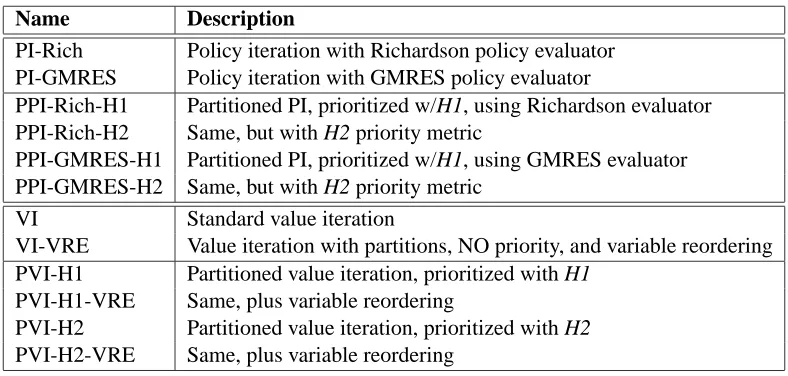
mini-Figure 7: On the left, the Kuhn triangulation of a (3d) cube. A d-dimensional hypercube is
tes-sellated (implicitly) into d! simplices. On the right, control of each(s,a)pair is tracked
until the resulting state s0 enters a new hypercube. Barycentric coordinates relative to
the enclosing simplex are computed, and are used to represent probabilistic transitions to vertices.
mum time optimal control problems, which are continuous time, and involve continuous action and state dimensions (these were discretized as described below). These control problems were selected because the number of states used in the discretization could be varied at will, while maintaining a constant expected degree, thus allowing us to generate families of highly related MDPs. The second set of problems were versions of the SysAdmin problem described by Guestrin et al. (2003). These are inherently discrete, stochastic problems with very dense transition matrices.
We will briefly describe the process used to discretize the control problems, but we note here that this process is tangential to the research focus of this paper. There are many other methods which could have been used to discretize the problems; naturally, this particular method introduces a bias with respect to the original problem, but since the solution engine simply expects a discrete MDP, the details of where it came from are somewhat irrelevant.
To discretize the space, we use the general numerical stochastic control techniques described by Kushner and Dupuis (2001); our specific implementation closely followed that of Munos and Moore (2002) (except that no variable discretization is used). Instead, the space is discretized once in the initialization phase. We refer the reader to their work for a complete description of the technique with comprehensive citations on component elements.
Figure 7 illustrates the discretization process. The state space is divided into hypercubes by regularly dividing each dimension, and a Kuhn triangulation is implemented (implicitly) inside of each hypercube. The use of Kuhn triangles is particularly appropriate because once discretized,
each state depends upon exactly d+1 other states. In addition, the combination of hypercubes and
Kuhn triangles has excellent space and time performance characteristics, which greatly accelerated the experimental cycle. The hypercubes completely tessellate the space, and the Kuhn triangles completely tessellate each hypercube. The vertices defining the hypercube grid are used as the states in the MDP. The transition matrix is computed by iterating over each vertex s. For each available action a, the system dynamics are integrated using Runge-Kutta and tracked until the resulting state
s0 enters a new hypercube. The barycentric coordinates of s0with respect to the enclosing simplex
mathematically equivalent to probabilistically jumping to a vertex: we approximate a deterministic continuous process by a stochastic discrete one” (emphasis in original).
Approximation of the value function is performed by computing exact values at each of the vertices, and interpolating the value across the interior of each hypercube. Interpolation is linear within each simplex. Since these problems are continuous time, a slightly different form of the value function equation was used:
Vt(s,a) = Z τ
0 γ
tR(s(t),a)dt+γτ
∑
s0∈S
Pr(s0|s(τ),a)max
a0∈AVt−1(s
0,a0)
whereτis the amount of time it took for s0to enter the new hypercube (or exit the state space), with
the convention thatτ=∞if s0never exited the original hypercube.
All results were obtained on a dual Opteron 246 with 8G of RAM. For partitioned solvers, there were always about 200 states in each partition, unless otherwise indicated. Results are deterministic, so wallclock tests were only run enough times to ensure accuracy.
3.1 Problem Details
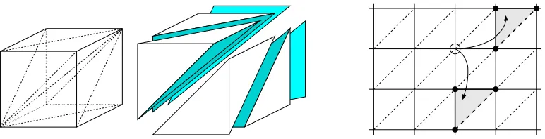
Mountain car (MCAR) is a two-dimensional minimum-time optimal control problem. A small car must rock back and forth until it gains enough momentum to carry itself up to the top of the hill (see Figure 8). In order to receive any reward, the car must exit the state space on the right-hand side (positive position), with a velocity close to zero. In order to make results more comparable to the other problems studied, the reward function was modified from the traditional gradient reward to be a single-point reward: the agent received a reward only upon exiting the state space with a velocity (within a threshold) of zero. This did not substantially change the shape of the resulting
value function. The state space is defined by position (x∈[−1,1]) and velocity ( ˙x∈[−4,4]).
The single-arm pendulum (SAP) is also a two dimensional minimum time optimal control prob-lem. The agent has two actions available (bang-bang control is sufficient for this problem) repre-senting positive and negative torques applied to rotating pendulum, which the agent must learn to swing up and balance. Similar to MCAR, the agent cannot move the pendulum from the bottom to the top directly, but must learn to rock it back and forth. Rewards are zero everywhere but in the
balanced region. The state space is defined by the angle of the link (θ1) and the angular velocity of
the link ( ˙θ1∈[−15,15]). The two actions are±10 Newton.
The double-arm pendulum (DAP) is a four dimensional minimum time optimal control problem (see Figure 8). It is similar to SAP, except that there are two links. It is the second link which the agent must balance vertically, but it is a free-swinging link. This variant of DAP is different from the easier Acrobot problem, where force is applied at the junction between the two links (Sutton, 1996), and from a horizontal double-arm pendulum (where the main link rotates in the horizontal plane, and the secondary link rotates vertically with respect to the main link). This version of DAP is the complete swing-up-and-balance problem; other variants only treat the balancing aspect. Rewards are zero everywhere but in the balanced region. The state space is defined by the two
link angles (θ1,θ2) and their angular velocities ( ˙θ1∈[−10,10]radians/s, ˙θ2∈[−15,15]radians/s).
Values outside these ranges are almost impossible to achieve, and are not necessary for the optimal
policy. The two actions are±10 Newton.
1 O
O1
O2 O2
Goal
Resistance
Thrust
Gravity
Figure 8: The left figure shows the MCAR problem (figure adapted from Munos and Moore, 2002). The car must rock itself back and forth to generate enough momentum to exit the state space. The state space is described by the position and velocity of the car. The right figure shows the DAP problem. The agent must swing the secondary link into the vertical
position and keep it there. The state space is described by four variables:θ1,θ2, ˙θ1and
˙
θ2. The same dynamics are used for the SAP problem.
each timestep, the administrator is paid proportionally to the number of machines that are on-line; the goal of the problem is to maximize the amount of money made. The state space is a binary vector, with each bit representing whether or not a machine is working. Machines fail with a fixed probability, with a failed machine increasing the probability of failure of any machine connected to
it. The administrator has n+1 actions available: action i corresponds to rebooting machine i, and
action n+1 means that nothing is rebooted. A rebooted machine is guaranteed to be working on the
next timestep. We used a network of 10 machines, connected in a ring topology; other network sizes were tested, with substantially similar results. See the paper by Guestrin et al. (2003) for specifics on generating the transition probabilities.
4. Results
4.1 Positive Results
Figures 9, 10 and 11 show that the enhancements constituting GPS clearly accelerate normal value and policy iteration for the SAP problem; substantially similar results were obtained for the MCAR problem. The gains were even better for the DAP problem, as shown in Figures 12 and 13, although the enhancements that worked the best on SAP and MCAR were different than the enhancements that worked the best on DAP. To solve a 160,000 state version of SAP, for example, VI required about 23 seconds, but PVI-H2-VRE required about 1.24 seconds. For a 6.25 million state version of DAP, VI required 110.64 seconds, but PVI-H1 required only 8.28 seconds. Similar performance gains were observed by enhancing policy iteration: PI-Rich and PI-GMRES solved the 6.25 million state DAP in about 250 seconds each; the partitioned, prioritized variants ranged in times between 12.53 and 22.77 seconds. It is also interesting to note that GPS solved both MCAR and SAP in about the same amount of time for any given discretization, even though they represent very different problems (in the sense that value information flows through them very differently).
The H2 metric usually exhibited better behavior than the H1 metric; the only exception was the DAP problem (this is discussed in the next section). The results also demonstrate that, while solving the control problems, the relative advantages of the enhancements were consistent as the problem size changed. This could be due to the fact that although the discretization level is changing, other fundamental properties of the MDP are not: the expected degree of any vertex is constant, the number of actions is very small, and there is only one reward in the system.
Variable reordering was almost always very effective on these control problems. In most exper-iments, reordering reduced time and backups by at least a factor of 2, and even in the cases when it did not help, we never saw a situation where it hurt in any statistically significant way. VRE thus appears to be a good enhancement, considering the low overhead and ease of implementation.
An additional advantage of prioritization is that some of the prioritized algorithms never pro-cessed certain states in the MCAR problem. Figure 16 demonstrates this graphically: large regions of the state space (indicated by a dark blue color) were never processed, because the agent can never reach the goal state from them. This is a significant result from a practical standpoint: no additional code or information about the problem was necessary, but a full 19% of the state space was never processed. This behavior manifested itself in the algorithm by a priority of zero that never changed. For all policy iteration variants, the Richardson iteration subsolver often outperformed the GM-RES subsolver. This is surprising, since Krylov methods are generally considered superior to their more naive counterparts. It is possible that the use of preconditioning may show GMRES in a more positive light, but such experiments are left to future research. We consider this a positive result because it indicates that using “naive” algorithms such as Modified Policy Iteration (Puterman and Shin, 1978) (which interleaves rounds of policy improvement with rounds of value iteration) may not be such a bad idea after all; the use of more sophisticated general matrix solvers may not be very fruitful because of the extremely specific type of matrix that is used in RL problems.
To validate the resulting policies from GPS, a 75,000,000 state version of DAP was run (an empirically determined minimum resolution needed for an effective control policy). This was done in the continuous domain by overlaying the discretization structure on the original space. Policies are exact at the vertices, so distance-weighted vertex voting was used to generate policies inside
each simplex. A very good result is that GPS solved it (toε=0.0001) in only about four hours. The
one third as fast as the Opteron used in all of the other experiments, and is a shared machine which is always heavily used.
4.2 Negative Results
The most significant negative result is the poor performance of GPS on the SysAdmin problem. Figure 14 shows some representative results: the best performers are standard PI and VI, and the worst are any GPS variant (except, of course, the variants which used only variable reordering; these showed slightly improved performance). As it turns out, SysAdmin is an example of the theoretically worst-case performance for GPS when compared to standard methods, and therefore represents the other extreme of the performance spectrum.
The problem lies in state interdependence. The transition matrix of this problem is extremely dense: under any policy, there is a non-zero probability of transitioning from any state to 50% of all of the other states. This is problematic for two reasons: first, the reprioritization calculations are very expensive, and second, the problem is not amenable to a divide-and-conquer strategy. Instead, this problem is like the one shown in Figure 2, where the best solution is a round-robin backup ordering. Thus, all of the overhead associated with maintaining priorities is pure overhead, in the sense that solution times would have been just as good without the effort.
The negative results are therefore not all that surprising, but deserve more quantification. A theoretical worst-case scenario for GPS can be estimated by considering a fully connected MDP
(Pr(s0|s,a)=6 0 ∀s,a,s0). The two critical factors in the reprioritization overhead are 1) the fact
that backing up a state is costly, which is true for any algorithm but which additionally implies
that recomputing Ht is costly, and 2) the fact that every state is dependent upon every other state,
implying that|SDP(p)|will be large for all p, and that Ht will need to be recomputed for a large
number of states. The very worst case occurs when just one state is included in each partition. Assume that just one backup per state s is needed to solve a partition. Then, to reprioritize dependent
partitions, we must recompute the priority for every dependent state (O(|S|)), by recomputing Ht(s),
which costs O(|S||A|). This incurs O(|S|2|A|)overhead per backup. Using fewer partitions helps, but
even then performance is worse than that of normal VI, because the same O(|S|2|A|)reprioritization
overhead is incurred whenever a partition is solved. The extra overhead is not justified when a round-robin method works just as well.
Additional experiments were conducted to discover which features of SysAdmin lead to the poor performance. These involved reducing the number of available actions, pruning low-probability transitions, testing various partition sizes, etc. GPS still performed poorly on these modified prob-lems. The current hypothesis is that all versions of SysAdmin considered still exhibit the same basic interdependence, which means that it is difficult to partition the problem cleanly, which implies that solving one partition before moving on to the next is not the best strategy. This leads to the fol-lowing general conclusion: highly interdependent states must be solved concurrently; spending too much time solving in isolation any one part of a problem which is highly interdependent on another part is wasted effort. This suggests that a better strategy for future versions of GPS may be to solve
each partition inexactly, instead of to withinε, but such an algorithm is left to future research.
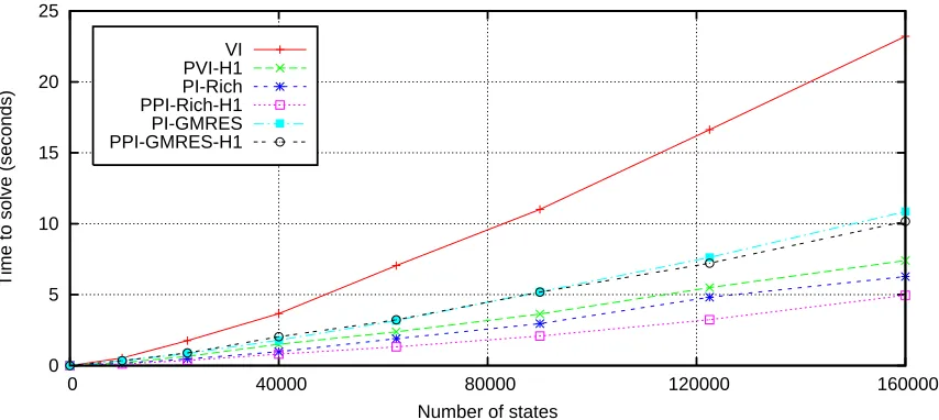
0 5 10 15 20 25
0 40000 80000 120000 160000
Time to solve (seconds)
Number of states VI
PVI-H1 PI-Rich PPI-Rich-H1 PI-GMRES PPI-GMRES-H1
Figure 9: Impact of using the H1 metric on the SAP problem. The y axis is time to solve in seconds (lower is better), and the x axis is the number of states used to discretize the problem. The reader should compare VI to PVI-H1, PI-Rich to PPI-Rich-H1, etc. These results show that using partitioning and prioritization with H1 always improves performance on this problem (although it does not improve by much between PI-GMRES and PPI-GMRES-H1). The improvement is especially large for VI. Partitions were generated using METIS.
GMRES outperforming Richardson, as well as H1 outperforming H2. In both sets of experiments, the largest performance gain seems to be due to the general idea of prioritization and partitioning; the specific variant of GPS used does not affect performance proportionately as much. Figure 12 also shows that, for a small number of states, VI slightly outperformed any GPS variant. Since each
state always depends on d+1 other states, the graph diameter of these problems may be smaller.
Neither our priority metrics, our variable reordering algorithm, nor our partitioning methods are optimal. For example, Figure 15 clearly shows that graph-based partitioning is not as effective as partitions based on geometrical information. Although the minimum-cut partitioning problem is NP-complete, it is unlikely that the suboptimality in our partitioning is what causes the poor performance; a more likely explanation is that we are partitioning based on the wrong criteria. Figure 5 shows that H2-VRE/200 performs fewer backups than H2-VRE/1. With PVI-H2-VRE/1, backups are executed in strict priority order, but with PVI-H2-VRE/200, backups are executed in an order that is partly due to the priority metric, and partly due to variable reordering. This fact implies that H2 generates a suboptimal ordering.
0 5 10 15 20 25
0 40000 80000 120000 160000
Time to solve (seconds)
Number of states VI
PVI-H2 PI-Rich PPI-Rich-H2 PI-GMRES PPI-GMRES-H2
Figure 10: Impact of using the H2 metric on the SAP problem. The results show that using par-titioning and prioritization with H2 always improves performance. In contrast to the previous figure, it substantially improves PI-GMRES. Partitions were generated using METIS.
0 5 10 15 20 25
0 40000 80000 120000 160000
Time to solve (seconds)
Number of states VI
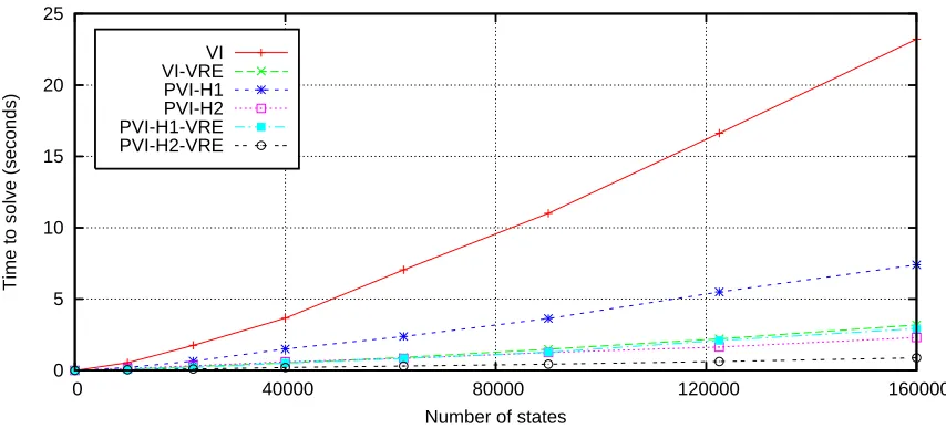
VI-VRE PVI-H1 PVI-H2 PVI-H1-VRE PVI-H2-VRE
0 20 40 60 80
0 5e+06 1e+07 1.5e+07 2e+07 2.5e+07
Time to solve (seconds)
Number of states
VI VI VRE PVI H1 PVI H1 VRE PVI H2 PVI H2 VRE
Figure 12: Results of the value iteration algorithms on the DAP problem. The results contrast some-what with the results for MCAR and SAP: H1 outperformed H2, and VRE negatively affected performance. However, any GPS variant greatly outperformed standard VI, with or without VRE. Partitions were generated using geometrical information.
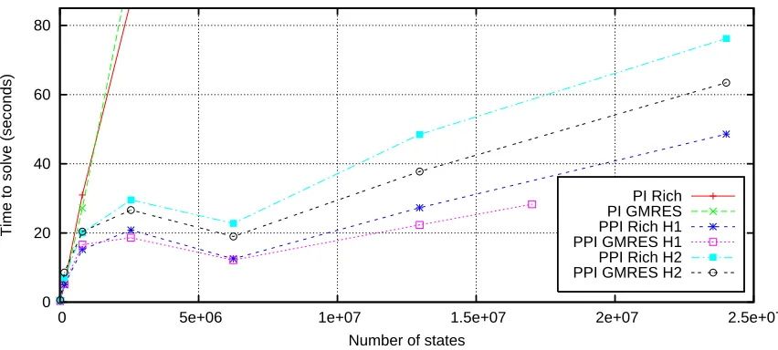
0 20 40 60 80
0 5e+06 1e+07 1.5e+07 2e+07 2.5e+07
Time to solve (seconds)
Number of states
PI Rich PI GMRES PPI Rich H1 PPI GMRES H1 PPI Rich H2 PPI GMRES H2
20 40 60 80 100
1 10 100
Time to solve (seconds)
Number of partitions
VI PI Rich PI GMRES PVI H1 PVI H2 VRE
Figure 14: Performance on the SysAdmin-10 problem, as a function of the number of partitions used. Only a representative sample of all algorithms is shown. The results contrast sharply with previous results: VI and PI dramatically outperform GPS variants, and adding partitions never helps any algorithm. VRE barely affects performance. Partitions were generated using METIS.
0.1 1 10 100
1 10 100 1000 10000
Time to solve (seconds)
Number of partitions Geometrical
Uniform Average Max
Figure 16: The MCAR control policy. Green (light gray) is positive thrust, red (medium gray) is negative thrust, and dark blue (dark gray) indicates that the partition was never pro-cessed. On the left: using one state per partition, the resolution of the unvisited states is very high, and corresponds exactly to the discontinuities in the value function. On the right: same, but using 100 states per partition. A partition can be skipped only if all of the states inside can be skipped.
5. Related Work
This work is about the efficient backpropagation of correct value function estimates. Other re-searchers who have investigated similar issues of efficiency have produced results that are tangible and compelling, but their algorithms are not directly comparable to ours because they have been developed in the context of on-line, model-free learning. Our algorithms, in contrast, explicitly assume the availability of a complete model.
The difference in these domains is significant and shifts the emphasis of the work. Model-free algorithms do not have the luxury of executing backups to states they have not visited; model-based algorithms, in contrast, can execute backups to any state, in any order. This fact frees us to examine different types of questions. For example, most model-free algorithms must content themselves with backpropagating information along experience traces, but there is no reason to suppose that an experience trace (played in any order) represents an optimal sequence of backups. It is a surrogate for what is truly desired: the ability to digest the consequences of corrected value function estimates as quickly and thoroughly as possible, throughout the entire problem. Thus, instead of examining questions related to maximizing the utility of experience traces, this work examines questions related to finding globally optimal backup sequences.
There are three primary classes of methods that researchers have used to accelerate the back-propagation of correct value information. Algorithmically, these methods form a poor basis for comparison, but conceptually, they illustrate several important points.
First is the class of trace propagation methods, such as TD(λ) (Sutton, 1988), Q(λ) (Peng and
Williams, 1994), SARSA(λ) (Rummery and Niranjan, 1994), Fast Q(λ) (Reynolds, 2002) and
up states in a principled order (that is, backwards) and by only backing up a subset of all states. These ideas of principled ordering and partial sweeps are central in this work.
Second, there are forced generalization methods, such as Eligibility Traces (Singh and Sutton, 1996), PQ-learning (Zhu and Levinson, 2002) and Propagation-TD (Preux, 2002). These methods attempt to compute the value for a state based on information that was not directly associated with an experience trace. States selected for backup may have been part of a previous experience trace, or may have a geometrical or geodesic relationship to states along the actual trace (this happens implicitly with function approximators, but is forced to happen explicitly in these tabular methods). Third, there are prioritized computation methods, such as Prioritized Sweeping (Moore and Atkeson, 1993) and Queue-DYNA (Peng and Williams, 1993). These methods order the backups in a principled way by constructing priority queues based on Bellman error. The idea of prioritizing backups is also central to our paper, but these methods raise many questions that merit further study. It is from these questions that our work springs.
Other researchers have considered extensions to the three basic classes previously enumerated, but the extensions do not match our domain of interest. For example, Andre et al. (1998) propose a continuous extension to Prioritized Sweeping, and Zhang and Zhang (2001) discuss a method for accelerating the convergence of value iteration in POMDPs. It is also well known that the dual of any MDP can be solved by linear programming. However, Littman et al. (1995) point out that “existing algorithms for solving LPs with provable polynomial-time performance are impractical for most MDPs. Practical algorithms for solving LPs based on the simplex method appear prone to the same sort of worst-case behavior as policy iteration and value iteration.” Guestrin et al. (2003) present efficient algorithms for solving factored MDPs, but the efficiency they describe relies on closed-form expressions for state spaces that are never explicitly enumerated. Gordon (1999) provides a thorough survey of other MDP solution techniques, such as state aggregation, interpolated value iteration, approximate policy iteration, policies without values, etc.
6. Conclusions and Future Research
Based on our observations, there are several important conclusions which clarify directions for future research. In the quest for an optimal sequence of backups, the gains to be had from prioritized computation are real and compelling, but there is a lack of understanding as to what constitutes optimality and how it can be achieved. A better understanding of why GPS works is needed: more principled approaches to selecting priority metrics, reordering methods, and partitioning schemes are essential. Ideally, such principled methods would all be combined in a unified architecture.
Partitioning with a priority metric seems to be the most important improvement. Even though we observed that our partitioning criteria was suboptimal, and that our reordering algorithm was suboptimal, and that both H1 and H2 are suboptimal, the fact that they were not perfect seemed to make less of a difference than the fact that we used them at all. This was shown clearly by DAP: the addition of VRE and the specific priority metric used did not affect things proportionately as much as the initial use of partitions.
ma-trices, strongly/weakly connected component analyses, etc. When do our enhancements work well? The rule of thumb seems to be “on problems with large diameter;” there is also evidence that they work well on problems with sparse rewards and a sparse transition matrix. We conclude that perhaps the control problems selected show GPS in its very best light – however, it was only GPS which made it possible for us to solve a 75,000,000, explicitly enumerated discrete state MDP. Without question, the algorithms are effective on certain types of problems.
More generally, the results indicate that dramatically improved performance is possible for al-gorithms that exploit problem-specific structure in an intelligent way. This motivates research into new types of representations (and companion algorithms) that are designed from the beginning with efficiency in mind. There are also many improvements that could be made using current ideas. For example, variable reordering can be considered a surrogate for an intra-partition priority metric. In the same way that partitioning a problem alleviates suboptimal backups, partitioning a partition might improve efficiency. The choice of a single-level partitioning scheme was arbitrary; perhaps a better solution is to generate a continuum of partitions with priority metrics at each level.
Overall, the results of this work have improved our ability to experiment with RL problems and have opened the doors of several fascinating avenues of research. At the very least, this work has enabled certain very large MDPs to be solved in tractable amounts of time and space, which would not have been possible otherwise; hopefully, this advance will allow researchers to design and tackle ever larger and more relevant problems. But the results also indicate that there are strong possibilities for even more efficient solution methods in the future, some of which may be radically different than anything considered to date, and which may enable even more intelligent systems to be created.
On-Line Appendix
The reader is encouraged to refer to
http://aml.cs.byu.edu/papers/prioritization methods/
for additional multi-media materials. Several videos are available which graphically demonstrate the different backup orders imposed by the different priority metrics. The GPS source code is also available for download.
Acknowledgments
The authors wish to thank Todd Peterson, Michael Goodrich, Dan Ventura and Martha Wingate for their patient revisions and cogent suggestions. They would also like to thank the anonymous reviewers for their attention to detail and excellent feedback.
David Wingate is supported under a National Science Foundation Graduate Research Fellow-ship.
References
David Andre, Nir Friedman, and Ronald Parr. Generalized prioritized sweeping. Advances in
Neural Information Processing Systems, 10:1001–1007, 1998.
Richard Barrett, Michael Berry, Tony F. Chan, James Demmel, June Donato, Jack Dongarra, Victor Eijkhout, Roldan Pozo, Charles Romine, and Henk Van der Vorst. Templates for the Solution of
Linear Systems: Building Blocks for Iterative Methods, 2nd Edition. SIAM, Philadelphia, PA,
1994.
Andrew G. Barto, S. J. Bradtke, and Satinder P. Singh. Learning to act using real-time dynamic programming. Artificial Intelligence, 72(1):81–138, 1995.
Dimitri P. Bertsekas. Distributed dynamic programming. IEEE Transactions on Automatic Control, 27:610–616, 1982.
Dimitri P. Bertsekas. Distributed asynchronous computation of fixed points. Mathematics
Program-ming, 27:107–120, 1983.
Dimitri P. Bertsekas and John Tsitsiklis. Neuro-Dynamic Programming. Athena Scientific, Belmont, MA, 1996.
Dimitri P. Bertsekas and John N. Tsitsiklis. Parallel and Distributed Computation: Numerical
Methods. Prentice-Hall, Englewood Cliffs, NJ, 1989.
Thomas Dean and Robert Givan. Model minimization in Markov Decision Processes. In
Proceed-ings of The Fourteenth National Conference on Artificial Intelligence, pages 106–111, 1997.
Geoffrey J. Gordon. Approximate Solutions to Markov Decision Processes. PhD thesis, Carnegie Mellon University, Pittsburgh, PA, 1999.
Carlos Guestrin, Daphne Koller, Ronald Parr, and Shobha Venkataraman. Efficient solution algo-rithms for factored MDPs. Journal of Artificial Intelligence Research, 19:399–468, 2003.
Vijaykumar Gullapalli and Andrew G. Barto. Convergence of indirect adaptive asynchronous value iteration algorithms. Advances in Neural Information Processing Systems, 6:695–702, 1994.
George Karypis and Vipin Kumar. Multilevel k-way partitioning scheme for irregular graphs.
Jour-nal of Parallel and Distributed Computing, 48:96–129, 1998.
Michael J. Kearns and Satinder P. Singh. Near-optimal reinforcement learning in polynomial time.
Machine Learning, 49:209–232, 2002.
Donald E. Knuth. The Stanford GraphBase: A Platform for Combinatorial Computing. ACM Press, New York, NY, 1993.
Harold J. Kushner and Paul Dupuis. Numerical methods for stochastic control problems in
contin-uous time, Second Edition. Springer-Verlag, New York, NY, 2001.
Michael L. Littman, Thomas L. Dean, and Leslie P. Kaelbling. On the complexity of solving Markov Decision Problems. In Proceedings of the Eleventh Annual Conference on Uncertainty