Generalization Bounds for the Area Under the ROC Curve

(1)

Generalization Bounds for the Area Under the ROC Curve

∗

Shivani Agarwal [email protected]

Department of Computer Science

University of Illinois at Urbana-Champaign 201 North Goodwin Avenue

Urbana, IL 61801, USA

Thore Graepel [email protected]

Ralf Herbrich [email protected]

Microsoft Research 7 JJ Thomson Avenue Cambridge CB3 0FB, UK

Sariel Har-Peled [email protected]

Dan Roth [email protected]

Department of Computer Science

University of Illinois at Urbana-Champaign 201 North Goodwin Avenue

Urbana, IL 61801, USA

Editor: Michael I. Jordan

Abstract

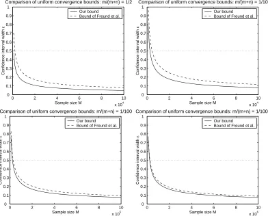
We study generalization properties of the area under the ROC curve (AUC), a quantity that has been advocated as an evaluation criterion for the bipartite ranking problem. The AUC is a different term than the error rate used for evaluation in classification problems; consequently, existing generaliza-tion bounds for the classificageneraliza-tion error rate cannot be used to draw conclusions about the AUC. In this paper, we define the expected accuracy of a ranking function (analogous to the expected error rate of a classification function), and derive distribution-free probabilistic bounds on the deviation of the empirical AUC of a ranking function (observed on a finite data sequence) from its expected accuracy. We derive both a large deviation bound, which serves to bound the expected accuracy of a ranking function in terms of its empirical AUC on a test sequence, and a uniform convergence bound, which serves to bound the expected accuracy of a learned ranking function in terms of its empirical AUC on a training sequence. Our uniform convergence bound is expressed in terms of a new set of combinatorial parameters that we term the bipartite rank-shatter coefficients; these play the same role in our result as do the standard VC-dimension related shatter coefficients (also known as the growth function) in uniform convergence results for the classification error rate. A compar-ison of our result with a recent uniform convergence result derived by Freund et al. (2003) for a quantity closely related to the AUC shows that the bound provided by our result can be considerably tighter.

Keywords: generalization bounds, area under the ROC curve, ranking, large deviations, uniform

convergence

(2)

1. Introduction

In many learning problems, the goal is not simply to classify objects into one of a fixed number of classes; instead, a ranking of objects is desired. This is the case, for example, in information retrieval problems, where one is interested in retrieving documents from some database that are ‘relevant’ to a given query or topic. In such problems, one wants to return to the user a list of documents that contains relevant documents at the top and irrelevant documents at the bottom; in other words, one wants a ranking of the documents such that relevant documents are ranked higher than irrelevant documents.

The problem of ranking has been studied from a learning perspective under a variety of settings (Cohen et al., 1999; Herbrich et al., 2000; Crammer and Singer, 2002; Freund et al., 2003). Here we consider the setting in which objects come from two categories, positive and negative; the learner is given examples of objects labeled as positive or negative, and the goal is to learn a ranking in which positive objects are ranked higher than negative ones. This captures, for example, the information retrieval problem described above; in this case, the training examples given to the learner consist of documents labeled as relevant (positive) or irrelevant (negative). This form of ranking problem corresponds to the ‘bipartite feedback’ case of Freund et al. (2003); for this reason, we refer to it as the bipartite ranking problem.

Formally, the setting of the bipartite ranking problem is similar to that of the binary classification problem. In both problems, there is an instance space

X

from which instances are drawn, and a set of two class labels

Y

which we take without loss of generality to be

Y

=_{−1,+1_}. One is given a finite sequence of labeled training examples S= ((x1,y1), . . . ,(xM,yM))∈(

X

×

Y

)M, and the goal is to learn a function based on this training sequence. However, the form of the function to be learned in the two problems is different. In classification, one seeks a binary-valued function h :

X

_→

Y

that predicts the class of a new instance in

X

. On the other hand, in ranking, one seeks a real-valued function f :

X

→R_{that induces a ranking over}

_X

_{; an instance that is assigned a higher value by f}

is ranked higher than one that is assigned a lower value by f .

What is a good classification or ranking function? Intuitively, a good classification function should classify most instances correctly, while a good ranking function should rank most instances labeled as positive higher than most instances labeled as negative. At first thought, these intuitions might suggest that one problem could be reduced to the other; that a good solution to one could be used to obtain a good solution to the other. Indeed, several approaches to learning ranking functions have involved using a standard classification algorithm that produces a classification function h of the form h(x) =θ(fh(x))for some real-valued function fh:

X

→R, where

θ(u) =

1 if u>0

−1 otherwise , (1)

and then taking fhto be the desired ranking function.1 However, despite the apparently close relation between classification and ranking, on formalizing the above intuitions about evaluation criteria for classification and ranking functions, it turns out that a good classification function may not always translate into a good ranking function.

(3)

1.1 Evaluation of (Binary) Classification Functions

In classification, one generally assumes that examples (both training examples and future, unseen examples) are drawn randomly and independently according to some (unknown) underlying distri-bution

D

over

X

×

Y

. The mathematical quantity typically used to evaluate a classification function

h :

X

→

Y

is then the expected error rate (or simply error rate) of h, denoted by L(h)and defined as

L(h) = EXY∼D

I_{h(X)6=Y} , (2)

where I_{·} denotes the indicator variable whose value is one if its argument is true and zero other-wise. The error rate L(h)is simply the probability that an example drawn randomly from

X

_×

Y

(according to

D

) will be misclassified by h; the quantity (1₋L(h))thus measures our intuitive notion of ‘how often instances are classified correctly by h’. In practice, since the distribution

D

is not known, the true error rate of a classification function cannot be computed exactly. Instead, the error rate must be estimated using a finite data sample. A widely used estimate is the empirical

error rate: given a finite sequence of labeled examples T= ((x1,y1), . . . ,(xN,yN))∈(

X

×

Y

)N, the empirical error rate of a classification function h with respect to T , which we denote by ˆL(h; T), is given by

ˆL(h; T) = 1

N

∑

i=1

I_{h(xi)6=yi}. (3)

When the examples in T are drawn randomly and independently from

X

×

Y

according to

D

, the sequence T constitutes a random sample. Much work in learning theory research has concentrated on developing bounds on the probability that an error estimate obtained from such a random sample will have a large deviation from the true error rate. While the true error rate of a classification function may not be exactly computable, such generalization bounds allow us to compute confidence intervals within which the true value of the error rate is likely to be contained with high probability.

1.2 Evaluation of (Bipartite) Ranking Functions

Evaluating a ranking function has proved to be somewhat more difficult. One empirical quantity that has been used for this purpose is the average precision, which relates to recall-precision curves. The average precision is often used in applications that contain very few positive examples, such as infor-mation retrieval. Another empirical quantity that has recently gained some attention as being well-suited for evaluating ranking functions relates to receiver operating characteristic (ROC) curves. ROC curves were originally developed in signal detection theory for analysis of radar images (Egan, 1975), and have been used extensively in various fields such as medical decision-making. Given a ranking function f :

X

_→R_{and a finite data sequence T} _{= ((}_x1,_y₁₎_{, . . . ,}₍_x_N_,_y_N₎₎_∈₍

_X

_×

_Y

₎N_{, the}

ROC curve of f with respect to T is obtained as follows. First, a set of N+1 classification functions

hi:

X

→

Y

, where 0≤i≤N, is constructed from f :

hi(x) = θ(f(x)−bi),

whereθ(_·)is as defined by Eq. (1) and

bi =   

f(xi) if 1≤i≤N

min 1≤j≤N f(xj)

(4)

The classification function h0classifies all instances in T as positive, while for 1≤i≤N, hiclassifies all instances ranked higher than xi as positive, and all others (including xi) as negative. Next, for each classification function hi, one computes the (empirical) true positive and false positive rates on

T , denoted by tpr_iand fpr_irespectively:

tpr_i = number of positive examples in T classified correctly by hi

total number of positive examples in T ,

fpr_i = number of negative examples in T misclassified as positive by hi

total number of negative examples in T .

Finally, the points(fpr_i,tpr_i)are plotted on a graph with the false positive rate on the x-axis and the true positive rate on the y-axis; the ROC curve is then obtained by connecting these points such that the resulting curve is monotonically increasing. It is the area under the ROC curve (AUC) that has been used as an indicator of the quality of the ranking function f (Cortes and Mohri, 2004; Rosset, 2004). An AUC value of one corresponds to a perfect ranking on the given data sequence (i.e., all positive instances in T are ranked higher than all negative instances); a value of zero corresponds to the opposite scenario (i.e., all negative instances in T are ranked higher than all positive instances). The AUC can in fact be expressed in a simpler form: if the sample T contains m positive and

n negative examples, then it is not difficult to see that the AUC of f with respect to T , which we

denote by ˆA(f ; T), is given simply by the following Wilcoxon-Mann-Whitney statistic (Cortes and Mohri, 2004):

ˆ

A(f ; T) = 1

mn

∑

{i:yi=+1}

∑

{j:yj=−1}

I_{f(xi)>f(xj)}+

1

2I{f(xi)=f(xj)}. (4)

In this simplified form, it becomes clear that the AUC of f with respect to T is simply the fraction of positive-negative pairs in T that are ranked correctly by f , assuming that ties are broken uniformly at random.2

There are two important observations to be made about the AUC defined above. The first is that the error rate of a classification function is not necessarily a good indicator of the AUC of a ranking function derived from it; different classification functions with the same error rate may pro-duce ranking functions with very different AUC values. For example, consider two classification functions h1,h2 given by hi(x) =θ(fi(x)),i=1,2, where the values assigned by f1,f2 to the in-stances in a sample T _∈(

X

×

Y

)8_{are as shown in Table 1. Clearly, ˆL}₍_h_{1; T}_{) =}_ˆL₍_h_{2; T}_{) =}_{2/8, but}

ˆ

A(f1; T) =12/16 while ˆA(f2; T) =8/16. The exact relationship between the (empirical) error rate of a classification function h of the form h(x) =θ(fh(x))and the AUC value of the corresponding ranking function fhwith respect to a given data sequence was studied in detail by Cortes and Mohri (2004). In particular, they showed that when the number of positive examples m in the given data sequence is equal to the number of negative examples n, the average AUC value over all possible rankings corresponding to classification functions with a fixed (empirical) error rate`is given by (1₋`), but the standard deviation among the AUC values can be large for large`. As the proportion of positive instances m/(m+n)departs from 1/2, the average AUC value corresponding to an error rate`departs from(1₋`), and the standard deviation increases further. The AUC is thus a different term than the error rate, and therefore requires separate analysis.

(5)

xi x1 x2 x3 x4 x5 x6 x7 x8

yi -1 -1 -1 -1 +1 +1 +1 +1

f1(xi) -2 -1 3 4 1 2 5 6

f2(xi) -2 -1 5 6 1 2 3 4

Table 1: Values assigned by two functions f1,f2to eight instances in a hypothetical example. The corresponding classification functions have the same (empirical) error rate, but the AUC values of the ranking functions are different. See text for details.

The second important observation about the AUC is that, as defined above, it is an empirical quantity that evaluates a ranking function with respect to a particular data sequence. What does the empirical AUC tell us about the expected performance of a ranking function on future examples? This is the question we address in this paper. The question has two parts, both of which are im-portant for machine learning practice. First, what can be said about the expected performance of a ranking function based on its empirical AUC on an independent test sequence? Second, what can be said about the expected performance of a learned ranking function based on its empirical AUC on the training sequence from which it is learned? The first part of the question concerns the large deviation behaviour of the AUC; the second part concerns its uniform convergence behaviour. Both are addressed in this paper.

We start by defining the expected ranking accuracy of a ranking function (analogous to the expected error rate of a classification function) in Section 2. Section 3 contains our large deviation result, which serves to bound the expected accuracy of a ranking function in terms of its empirical AUC on an independent test sequence. Our conceptual approach in deriving the large deviation result for the AUC is similar to that of (Hill et al., 2002), in which large deviation properties of the average precision were considered. Section 4 contains our uniform convergence result, which serves to bound the expected accuracy of a learned ranking function in terms of its empirical AUC on a training sequence. Our uniform convergence bound is expressed in terms of a new set of combinatorial parameters that we term the bipartite rank-shatter coefficients; these play the same role in our result as do the standard shatter coefficients (also known as the growth function) in uniform convergence results for the classification error rate. A comparison of our result with a recent uniform convergence result derived by Freund et al. (2003) for a quantity closely related to the AUC shows that the bound provided by our result can be considerably tighter. We conclude with a summary and some open questions in Section 5.

2. Expected Ranking Accuracy

We begin by introducing some additional notation. As in classification, we shall assume that all examples are drawn randomly and independently according to some (unknown) underlying distri-bution

D

over

X

×

Y

. The notation

D+

1 and

D

−1 will be used to denote the class-conditional distributions

D

X_|Y=+1 and

D

X_|Y=−1, respectively. We use an underline to denote a sequence, e.g.,

y_∈

Y

N _{to denote a sequence of elements in}

_Y

_{. We shall find it convenient to decompose a data} sequence T= ((x1,y1), . . . ,(xN,yN))∈(

X

×

Y

)Ninto two components, TX= (x1, . . . ,xN)∈

X

Nand

(6)

some label sequence y= (y1, . . . ,yN)∈

Y

N; this distribution is simply

D

y1×. . .×

D

yN.

3 _{If the} distri-bution is clear from the context it will be dropped in the notation of expectations and probabilities,

e.g., EXY ≡EXY∼D. As a final note of convention, we use T ∈(

X

×

Y

)N to denote a general data

sequence (e.g., an independent test sequence), and S∈(

X

×

Y

)M_{to denote a training sequence.} We define below a quantity that we term the expected ranking accuracy; the purpose of this quantity will be to serve as an evaluation criterion for ranking functions (analogous to the use of the expected error rate as an evaluation criterion for classification functions).

Definition 1 (Expected ranking accuracy) Let f :

X

→R_{be a ranking function on}

_X

_{. Define the}

expected ranking accuracy (or simply ranking accuracy) of f , denoted by A(f), as follows:

A(f) = EX_∼D+1,X0∼D−1

I_{_f₍_X₎_>_f₍_X0₎_}+

1

2I{f(X)=f(X0)}

. (5)

The ranking accuracy A(f)defined above is simply the probability that an instance drawn ran-domly according to

D+

1will be ranked higher by f than an instance drawn randomly according to

D

₋1, assuming that ties are broken uniformly at random; the quantity A(f)thus measures our intu-itive notion of ‘how often instances labeled as posintu-itive are ranked higher by f than instances labeled as negative’. As in the case of classification, the true ranking accuracy depends on the underlying distribution of the data and cannot be observed directly. Our goal shall be to derive generalization bounds that allow the true accuracy of a ranking function to be estimated from its empirical AUC with respect to a finite data sample. The following simple lemma shows that this makes sense, for given a fixed label sequence, the empirical AUC of a ranking function f is an unbiased estimator of the expected ranking accuracy of f :

Lemma 2 Let f :

X

_X

_{, and let y}_{= (}_y₁_{, . . . ,}_y_N₎_∈

_Y

N_{be a finite label}

sequence. Then

ETX|TY=y

_ˆ

A(f ; T) = A(f).

Proof Let m be the number of positive labels in y, and n the number of negative labels in y. Then from the definition of empirical AUC (Eq. (4)) and linearity of expectation, we have

E_T_X_|_T_Y₌_y_ˆ

A(f ; T) = 1

mn_{_i:y

∑

i=+1}

∑

{j:yj=−1}

EXi∼D+1,Xj∼D−1

I_{_f₍_X_i₎_>_f₍_X_j₎_}+1

2I{f(Xi)=f(Xj)}

= 1

mn_{_i:y

∑

i=+1}

∑

{j:yj=−1}

A(f)

= A(f).

3. Note that, since the AUC of a ranking function f with respect to a data sequence T∈(X×Y)N_{is independent of the}

actual ordering of examples in the sequence, our results involving the conditional distributionDTX|TY=yfor some label

sequence y= (y1, . . . ,yN)∈YNdepend only on the number m of positive labels in y and the number n of negative

labels in y. We choose to state our results in terms of the distributionDTX|TY=y≡Dy1×. . .×DyN only because this

is more general than stating them in terms ofDm

+1×D

n

(7)

We are now ready to present the main results of this paper, namely, a large deviation bound in Section 3 and a uniform convergence bound in Section 4. We note that our results are all distribution-free, in the sense that they hold for any distribution

D

over

X

×

Y

.

3. Large Deviation Bound for the AUC

In this section we are interested in bounding the probability that the empirical AUC of a ranking function f with respect to a (random) test sequence T will have a large deviation from its expected ranking accuracy. In other words, we are interested in bounding probabilities of the form

PAˆ(f ; T)−A(f) ≥ε

for given ε>0. Our main tool in deriving such a large deviation bound will be the following powerful concentration inequality of McDiarmid (1989), which bounds the deviation of any function of a sample for which a single change in the sample has limited effect:

Theorem 3 (McDiarmid, 1989) Let X1, . . . ,XN be independent random variables with Xk taking

values in a set Ak for each k. Letφ:(A1× ··· ×AN)→Rbe such that sup

xi∈Ai,x0k∈Ak

φ(x1, . . . ,x_N)−φ(x1, . . . ,x_k₋₁,x0_k,x_k₊₁, . . . ,x_N)

≤ c_k.

Then for anyε>0,

P_{|φ(X1, . . . ,XN)−E{φ(X1, . . . ,XN)}| ≥ε} ≤ 2e−2ε 2_/_∑N

k=1c2k.

Note that when X1, . . . ,XN are independent bounded random variables with Xk ∈[ak,bk]with probability one, andφ(X1, . . . ,XN) =∑Nk=1Xk, McDiarmid’s inequality (with ck =bk−ak) reduces to Hoeffding’s inequality. Next we define the following quantity which appears in several of our results:

Definition 4 (Positive skew) Let y= (y1, . . . ,yN)∈

Y

Nbe a finite label sequence of length N∈N.

Define the positive skew of y, denoted byρ(y), as follows:

ρ(y) = 1

N

∑

{i:yi=+1}

1. (6)

The following is the main result of this section:

Theorem 5 Let f :

X

→R_{be a fixed ranking function on}

_X

_{and let y}_{= (}_y₁_{, . . . ,}_y_N₎_∈

_Y

N _{be any}

label sequence of length N _∈N_{. Let m be the number of positive labels in y, and n}₌_N₋_{m the}

number of negative labels in y. Then for anyε>0,

PTX|TY=y

Aˆ(f ; T)−A(f)

≥ε ≤ 2e−2mnε 2_/₍_m₊_n₎

(8)

Proof Given the label sequence y, the random variables X1, . . . ,XN are independent, with each Xk taking values in

X

. Now, defineφ:

X

N_→_R_{as follows:}

φ(x1, . . . ,xN) = Aˆ(f ;((x1,y1), . . . ,(xN,yN))). Then, for each k such that yk= +1, we have the following for all xi,x0k∈

X

:

φ(x1, . . . ,x_N)−φ(x1, . . . ,x_k₋1,x0_k,x_k₊₁. . . ,x_N)

= 1

mn

_{_j:y

∑

j=−1}

I_{f(xk)>f(xj)}+

1

2I{f(xk)=f(xj)}

−

I_{f(x0_k)>f(xj)}+

1

2I{f(x0k)=f(xj)}

! ≤ _mn1 n

= 1

m.

Similarly, for each k such that yk=−1, one can show for all xi,x0_k∈

X

:

φ(x₁, . . . ,x_N)−φ(x₁, . . . ,x_k₋₁,x0_k,x_k₊₁. . . ,x_N) ≤

1

n.

Thus, taking ck=1/m for k such that yk= +1 and ck=1/n for k such that yk=−1, and applying McDiarmid’s theorem, we get for anyε>0,

PTX|TY=y

n

Aˆ(f ; T)−ETX|TY=y

_ˆ

A(f ; T) ≥ε

o

≤ 2e−2ε2/(m(m1)2+n(

1

n)2)

= 2e−2mnε2/(m+n). The result follows from Lemma 2.

We note that the result of Theorem 5 can be strengthened so that the conditioning is only on the numbers m and n of positive and negative labels, and not on the specific label vector y. From Theorem 5, we can derive a confidence interval interpretation of the bound that gives, for any 0<δ_≤1, a confidence interval based on the empirical AUC of a ranking function (on a random test sequence) which is likely to contain the true ranking accuracy with probability at least 1₋δ. More specifically, we have:

Corollary 6 Let f :

X

_X

_{and let y}_{= (}_y_{1, . . . ,}_y_N₎_∈

_Y

N _{be any}

label sequence of length N_∈N_{. Then for any 0}_<δ_≤_1,

P_T_X_|_T_Y₌_y (

Aˆ(f ; T)−A(f) ≥

s

ln 2_δ 2ρ(y)(1₋ρ(y))N

)

≤ δ.

(9)

We note that a different approach for deriving confidence intervals for the AUC has recently been taken by Cortes and Mohri (2005); in particular, their confidence intervals for the AUC are constructed from confidence intervals for the classification error rate.

Theorem 5 also allows us to obtain an expression for a test sample size that is sufficient to obtain, for given 0<ε,δ_≤1, anε-accurate estimate of the ranking accuracy withδ-confidence:

Corollary 7 Let f :

X

_X

_{and let 0}_<ε_,δ_≤_{1. Let y}_{= (}_y₁_{, . . . ,}_y_N₎_∈

Y

N _{be any label sequence of length N}_∈_N_{. If}

N _≥ ln

2

δ

2ρ(y)(1₋ρ(y))ε2,

then

PTX|TY=y

Aˆ(f ; T)−A(f)

≥ε ≤ δ.

Proof This follows directly from Theorem 5 by setting 2e−2ρ(y)(1−ρ(y))Nε2_≤δand solving for N.

The confidence interval of Corollary 6 can in fact be generalized to remove the conditioning on the label vector completely:

Theorem 8 Let f :

X

_X

_{and let N}_∈N_{. Then for any 0}_<δ_≤_1,

P_T_∼_DN

  

Aˆ(f ; T)−A(f) ≥

s

ln 2_δ 2ρ(TY)(1−ρ(TY))N

  

≤ δ.

Proof For T_∈(

X

_×

Y

)N_{and 0}_<δ_≤_{1, define the proposition}

Φ(T,δ) _≡   

Aˆ(f ; T)−A(f) ≥

s

ln 2_δ 2ρ(TY)(1−ρ(TY))N

   .

Then for any 0<δ_≤1, we have

PT{Φ(T,δ)} = ET

I_Φ(T,δ)

= ETY

n

ETX|TY=y

I_Φ(T,δ)

o

= ETY

n

PTX|TY=y{Φ(T,δ)}

o

≤ ETY{δ} (by Corollary 6)

= δ.

Note that the above ‘trick’ works only once we have gone to a confidence interval; an attempt to generalize the bound of Theorem 5 in a similar way gives an expression in which the final ex-pectation is not easy to evaluate. Interestingly, the above proof does not even require a factorized distribution

D

TY since it is built on a result for any fixed label sequence y. We note that the above

(10)

3.1 Comparison with Bounds from Statistical Literature

The AUC, in the form of the Wilcoxon-Mann-Whitney statistic, has been studied extensively in the statistical literature. In particular, Lehmann (1975) derives an exact expression for the variance of the Wilcoxon-Mann-Whitney statistic which can be used to obtain large deviation bounds for the AUC. Below we compare the large deviation bound we have derived above with these bounds obtainable from the statistical literature. We note that the expression derived by Lehmann (1975) is for a simpler form of the Wilcoxon-Mann-Whitney statistic that does not account for ties; therefore, in this section we assume the AUC and the expected ranking accuracy are defined without the terms that account for ties (the large deviation result we have derived above applies also in this setting).

Let f :

X

→R _{be a fixed ranking function on}

_X

_{and let y}_{= (}_y₁_{, . . . ,}_y_N₎_∈

_Y

N _{be any label}

sequence of length N_∈N_{. Let m be the number of positive labels in y, and n}₌_N₋_{m the number}

of negative labels in y. Then the variance of the AUC of f is given by the following expression (Lehmann, 1975):

σ2

A = VarTX|TY=y

_ˆ

A(f ; T)

= A(f)(1−A(f)) + (m−1)(p1−A(f)

2_{) + (}_n₋₁₎₍_p

2−A(f)2)

mn , (7)

where

p1 = PX1+,X2+∼D+1,X1−∼D−1 nn

f(X₁+)> f(X₁−)o_∩nf(X₂+)> f(X₁−)oo (8)

p2 = PX₁+∼D+1,X1−,X2−∼D−1 nn

f(X₁+)> f(X₁−)o_∩nf(X₁+)> f(X₂−)oo. (9) Next we recall the following classical inequality:

Theorem 9 (Chebyshev’s inequality) Let X be a random variable. Then for anyε>0,

P_{|X₋E_{X_{}| ≥}ε_{} ≤} Var{X}

ε2 .

The expression for the varianceσ2_Aof the AUC can be used with Chebyshev’s inequality to give the following bound: for anyε>0,

P_T_X_|_T_Y₌_y

Aˆ(f ; T)−A(f)

≥ε ≤ σ2

A

ε2 . (10)

This leads to the following confidence interval: for any 0<δ_≤1,

PTX|TY=y

Aˆ(f ; T)−A(f) ≥

σA

√_δ

≤ δ. (11)

It has been established that the AUC follows an asymptotically normal distribution. Therefore, for large N, one can use a normal approximation to obtain a tighter bound:

PTX|TY=y

Aˆ(f ; T)−A(f)

≥ε ≤ 2(1−Φ(ε/σ_A)), (12) whereΦ(_·)denotes the standard normal cumulative distribution function given byΦ(u) =Ru

0 e−z 2_/₂

dz/√2π. The resulting confidence interval is given by

PTX|TY=y

Aˆ(f ; T)−A(f)

(11)

The quantities p1and p2that appear in the expression forσ2_Ain Eq. (7) depend on the underlying distributions

D+

1and

D

₋1; for example, Hanley and McNeil (1982) derive expressions for p1and

p2 in the case when the scores f(X+) assigned to positive instances X+ and the scores f(X−) assigned to negative instances X− both follow negative exponential distributions. Distribution-independent bounds can be obtained by using the fact that the varianceσ2_A is at most (Cortes and Mohri, 2005; Dantzig, 1915; Birnbaum and Klose, 1957)

σ2 max =

A(f)(1₋A(f)) min(m,n) ≤

1

4 min(m,n). (14)

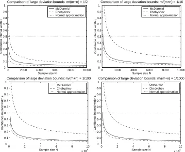
A comparison of the resulting bounds with the large deviation bound we have derived above using McDiarmid’s inequality is shown in Figure 1. The McDiarmid bound is tighter than the bound obtained using Chebyshev’s inequality. It is looser than the bound obtained using the normal ap-proximation; however, since the normal approximation is valid only for large N, for smaller values of N the McDiarmid bound is safer.

Of course, it should be noted that this comparison holds only in the distribution-free setting. In practice, depending on the underlying distribution, the actual variance of the AUC may be much smaller thanσ2_max; indeed, in the best case, the variance could be as small as

σ2 min =

A(f)(1₋A(f))

mn ≤

1

4mn. (15)

Therefore, one may be able to obtain tighter confidence intervals with Eqs. (11) and (13) by esti-mating the actual variance of the AUC. For example, one may attempt to estimate the quantities p1,

p2 and A(f)that appear in the expression in Eq. (7) directly from the data, or one may use resam-pling methods such as the bootstrap (Efron and Tibshirani, 1993), in which the variance is estimated from the sample variance observed over a number of bootstrap samples obtained from the data. The confidence intervals obtained using such estimates are only approximate (i.e., the 1₋δconfidence is not guaranteed), but they can often be useful in practice.

3.2 Comparison with Large Deviation Bound for Classification Error Rate

Our use of McDiarmid’s inequality in deriving the large deviation bound for the AUC of a ranking function is analogous to the use of Hoeffding’s inequality in deriving a similar large deviation bound for the error rate of a classification function (see, for example, Devroye et al., 1996, Chapter 8). The need for the more general inequality of McDiarmid in our derivation arises from the fact that the empirical AUC, unlike the empirical error rate, cannot be expressed as a sum of independent random variables. In the notation of Section 1, the large deviation bound for the classification error rate obtained via Hoeffding’s inequality states that for a fixed classification function h :

X

→

Y

and for any N∈N_{and any}ε>0,

PT∼DN

ˆL(h; T)−L(h)

≥ε ≤ 2e−2Nε 2

. (16)

(12)

0 2000 4000 6000 8000 10000 0

0.1 0.2 0.3 0.4 0.5 0.6 0.7 0.8 0.9 1

Comparison of large deviation bounds: m/(m+n) = 1/2

Sample size N

Confidence interval width

ε

McDiarmid Chebyshev Normal approximation

0 2000 4000 6000 8000 10000 0

0.1 0.2 0.3 0.4 0.5 0.6 0.7 0.8 0.9 1

Sample size N

ε

0 2 4 6 8 10

x 104 0

0.1 0.2 0.3 0.4 0.5 0.6 0.7 0.8 0.9 1

Sample size N

ε

0 2 4 6 8 10

x 105 0

0.1 0.2 0.3 0.4 0.5 0.6 0.7 0.8 0.9 1

Sample size N

ε

Figure 1: A comparison of our large deviation bound, derived using McDiarmid’s inequality, with large deviation bounds obtainable from the statistical literature (see Section 3.1). The plots are forδ=0.01 and show how the confidence interval sizeεgiven by the different bounds varies with the sample size N=m+n, for various values of m/(m+n).

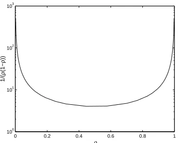
test sample size sufficient to obtain anε-accurate estimate of the expected error rate of a classifica-tion funcclassifica-tion with the same confidence. Forρ(y) =1/2, this means a sample size larger by a factor of 4; as the positive skewρ(y)departs from 1/2, the factor grows larger (see Figure 2).

Again, it should be noted that the above conclusion holds only in the distribution-free setting. Indeed, the varianceσ2_Lof the error rate (which follows a binomial distribution) is given by

σ2

L = VarT∼DN

ˆL(h; T) = L(h)(1−L(h))

N ≤

1

4N. (17)

(13)

0 0.2 0.4 0.6 0.8 1 100

101

102 103

ρ

1/(

ρ

(1−

ρ

))

Figure 2: The test sample size bound for the AUC, for positive skewρ_≡ρ(y)for some label se-quence y, is larger than the corresponding test sample size bound for the error rate by a factor of 1/(ρ(1₋ρ))(see text for discussion).

3.3 Bound for Learned Ranking Functions Chosen from Finite Function Classes

The large deviation result of Theorem 5 bounds the expected accuracy of a ranking function in terms of its empirical AUC on an independent test sequence. A simple application of the union bound allows the result to be extended to bound the expected accuracy of a learned ranking function in terms of its empirical AUC on the training sequence from which it is learned, in the case when the learned ranking function is chosen from a finite function class. More specifically, we have:

Theorem 10 Let

F

be a finite class of real-valued functions on

X

and let fS∈

F

denote the ranking

function chosen by a learning algorithm based on the training sequence S. Let y= (y1, . . . ,yM)∈

Y

M_{be any label sequence of length M}_∈_N_{. Then for any}_ε_>_0,

PSX|SY=y

Aˆ(f_S; S)−A(f_S)

≥ε ≤ 2|

F

|e−2ρ(y)(1−ρ(y))Mε 2

.

Proof For anyε>0, we have

P_S_X_|_S_Y₌_y

Aˆ(f_S; S)−A(f_S) ≥ε ≤ PSX|SY=y

max

f_∈F

Aˆ(f ; S)−A(f) ≥ε

≤

∑

f_∈F

PSX|SY=y

Aˆ(f ; S)−A(f)

≥ε (by the union bound)

≤ 2_|

F

_|e−2ρ(y)(1−ρ(y))Mε2 (by Theorem 5).

(14)

Corollary 11 Let

F

X

and let fS∈

F

Y

M_{be any label sequence of length M}_∈_N_{. Then for any 0}_<_δ_≤_1,

PSX|SY=y

(

Aˆ(f_S; S)−A(f_S) ≥

s

ln_|

F

|+ln 2_δ 2ρ(y)(1₋ρ(y))M

)

≤ δ.

F

X

and let fS∈

F

Y

M_{be any label sequence of length M}_∈_N_{. Then for any 0}_<_ε_,_δ_≤_{1, if}

M _≥ 1

2ρ(y)(1₋ρ(y))ε2

ln_|

F

|+ln

2 δ

,

then

PSX|SY=y

Aˆ(f_S; S)−A(f_S)

≥ε ≤ δ.

Theorem 13 Let

F

X

and let fS∈

F

function chosen by a learning algorithm based on the training sequence S. Let M_∈N_{. Then for any}

0<δ_≤1,

P_S_∼_DM

  

Aˆ(f_S; S)−A(f_S) ≥

s

ln_|

F

|+ln 2_δ 2ρ(SY)(1−ρ(SY))M

  

≤ δ.

The above results apply only to ranking functions learned from finite function classes. The general case, when the learned ranking function may be chosen from a possibly infinite function class, is the subject of the next section.

4. Uniform Convergence Bound for the AUC

In this section we are interested in bounding the probability that the empirical AUC of a learned ranking function fS with respect to the (random) training sequence S from which it is learned will have a large deviation from its expected ranking accuracy, when the function fS is chosen from a possibly infinite function class

F

. The standard approach for obtaining such bounds is via uniform convergence results. In particular, we have for anyε>0,

PAˆ(f_S; S)−A(f_S)

≥ε ≤ P (

sup f∈F

Aˆ(f ; S)−A(f) ≥ε

) .

(15)

₁

001 ½0 01 10½1 10½0 1½01 ½0 ½1 ½0 0½ ½½01 10½½ 1½½1 1½0½ ½1 ½½ ½½0½ ½½½1 ½0 ½½ ₀

110 ½1 10 01½0 01½1 0½10 ½1 ½0 ½1 1½ ½½10 01½½ 0½½0 0½1½ ½0 ½½ ½½1½ ½½½0 ½1 ½½

Table 2: Sub-matrices that cannot appear in a bipartite rank matrix.

4.1 Bipartite Rank-Shatter Coefficients

We define first the notion of a bipartite rank matrix; this is used in our definition of bipartite rank-shatter coefficients.

Definition 14 (Bipartite rank matrix) Let f :

X

_X

_{, let m}_,_n_∈N_{, and}

let x= (x1, . . . ,xm)∈

X

m, x0= (x01, . . . ,x0n)∈

X

n. Define the bipartite rank matrix of f with respect

to x,x0, denoted by Bf(x,x0), to be the matrix in{0,1₂,1}m×nwhose(i,j)-th element is given by

Bf(x,x0)

i j = I{f(xi)>f(x0j)}+

1

2I{f(xi)=f(x0j)} (18)

for all i_{∈ {}1, . . . ,m_}, j_{∈ {}1, . . . ,n_}.

Definition 15 (Bipartite rank-shatter coefficient) Let

F

be a class of real-valued functions on

X

, and let m,n∈N_{. Define the}₍_m_,_n₎_{-th bipartite rank-shatter coefficient of}

_F

_{, denoted by r}₍

_F

_,_m_,_n₎_,

as follows:

r(

F

,m,n) = max x∈Xm_,_x0_∈_Xn

Bf(x,x0)| f ∈

F

. (19)

Clearly, for finite

F

, we have r(

F

,m,n)_{≤ |}

F

|for all m,n. In general, r(

F

,m,n)_≤3mn for all m,n. In fact, not all 3mn matrices in _{0,1

2,1}

m×n _{can be realized as bipartite rank matrices.} Therefore, we have

r(

F

,m,n)_≤ψ(m,n),

where ψ(m,n) is the number of matrices in _{0,1 2,1}

m_×n _{that can be realized as a bipartite rank}

matrix. The numberψ(m,n)can be characterized in the following ways:

Theorem 16 Letψ(m,n)be the number of matrices in_{0,1 2,1}

m×n_{that can be realized as a}

bipar-tite rank matrix Bf(x,x0)for some f :

X

→R, x∈

X

m, x0∈

X

n. Then

1. ψ(m,n) is equal to the number of complete mixed acyclic(m,n)-bipartite graphs (where a mixed graph is one which may contain both directed and undirected edges, and where we define a cycle in such a graph as a cycle that contains at least one directed edge and in which all directed edges have the same directionality along the cycle).

2. ψ(m,n)is equal to the number of matrices in_{0,1₂,1_}m×n_{that do not contain a sub-matrix of}

any of the forms shown in Table 4.1.

Proof

(16)

{v0₁, . . . ,v0_n} be sets of m and n vertices respectively, and for any matrix B= [bi j]∈ {0,1₂,1}m×n, let E(B) denote the set of edges between V and V0 given by E(B) =_{(vi ← v0j) | bi j =1} ∪

{(vi → v0j) |bi j =0} ∪ {(vi — v0j) | bi j = 1₂}. Define the mapping G :{0,1₂,1}m×n →

G

(m,n) as follows:

G(B) = (V_∪V0,E(B)).

Then clearly, G is a bijection that puts the sets_{0,1 2,1}

m×n_and

_G

₍_m_,_n₎_{into one-to-one} correspon-dence. We show that a matrix B_{∈ {}0,1

2,1}m×ncan be realized as a bipartite rank matrix if and only if the corresponding bipartite graph G(B)_∈

G

(m,n)is acyclic.

First suppose B=Bf(x,x0)for some f :

X

→R, x∈

X

m, x0∈

X

n, and let if possible G(B)contain a cycle, say

(vi1 ←v0j1 — vi2 — v0j2 — . . . — vik — v0jk— vi1).

Then, from the definition of a bipartite rank matrix, we get

f(xi1)<f(x0j1) = f(xi2) =f(x0j2) =. . .= f(xik) = f(x0jk) = f(xi1),

which is a contradiction.

To prove the other direction, let B_{∈ {}0,1 2,1}

m_×n_{be such that G}₍_B₎_{is acyclic. Let G}₀₍_B₎_denote

the directed graph obtained by collapsing together vertices in G(B)that are connected by an undi-rected edge. Then it is easily verified that G0(B)does not contain any directed cycles, and therefore there exists a complete order on the vertices of G0(B)that is consistent with the partial order defined by the edges of G0(B)(topological sorting; see, for example, Cormen et al., 2001, Section 22.4). This implies a unique order on the vertices of G(B) (in which vertices connected by undirected edges are assigned the same position in the ordering). For any x_∈

X

m_{, x}₀_∈

_X

n_{, identifying x,}_x₀ with the vertex sets V,V0of G(B)therefore gives a unique order on x1, . . . ,xm,x01, . . . ,x0n. It can be verified that defining f :

X

→R_{such that it respects this order then gives B}₌_B_f₍_x,x0₎_.

Part 2. Consider again the bijection G :_{0,1 2,1}

m_×n _→

_G

₍_m_,_n₎_{defined in Part 1 above. We show}

that a matrix B∈ {0,1

2,1}m×ndoes not contain a sub-matrix of any of the forms shown in Table 4.1 if and only if the corresponding bipartite graph G(B)_∈

G

(m,n)is acyclic; the desired result then follows by Part 1 of the theorem.

We first note that the condition that B∈ {0,1

2,1}m×nnot contain a sub-matrix of any of the forms shown in Table 4.1 is equivalent to the condition that the corresponding mixed(m,n)-bipartite graph

G(B)_∈

G

(m,n)not contain any 4-cycles.

Now, to prove the first direction, let B∈ {0,1

2,1}m×n not contain a sub-matrix of any of the forms shown in Table 4.1. As noted above, this means G(B)does not contain any 4-cycles. Let, if possible, G(B)contain a cycle of length 2k, say

Now consider vi1,v0j2. Since G(B) is a complete bipartite graph, there must be an edge between these vertices. If G(B)contained the edge(vi1 →v0j2), it would contain the 4-cycle

(vi1 ←v0j1 — vi2 — v0j2 ←vi1),

which would be a contradiction. Similarly, if G(B)contained the edge(vi1 — v0j2), it would contain the 4-cycle

(17)

which would again be a contradiction. Therefore, G(B)must contain the edge(vi1←v0j2). However, this means G(B)must contain a 2(k₋1)-cycle, namely,

By a recursive argument, we eventually get that G(B)must contain a 4-cycle, which is a contradic-tion.

To prove the other direction, let B_{∈ {}0,1 2,1}

m×n_{be such that G}₍_B₎_{is acyclic. Then it follows} trivially that G(B)does not contain a 4-cycle, and therefore, by the above observation, B does not contain a sub-matrix of any of the forms shown in Table 4.1.

We discuss further properties of the bipartite rank-shatter coefficients in Section 4.3; we first present below our uniform convergence result in terms of these coefficients.

4.2 Uniform Convergence Bound

The following is the main result of this section:

Theorem 17 Let

F

X

, and let y= (y1, . . . ,yM)∈

Y

Mbe any

label sequence of length M_∈N_{. Let m be the number of positive labels in y, and n}₌_M₋_{m the}

number of negative labels in y. Then for anyε>0,

PSX|SY=y

( sup f∈F

Aˆ(f ; S)−A(f) ≥ε

)

≤ 4_·r(

F

,2m,2n)_·e−mnε2/8(m+n)

= 4_·r

F

,2ρ(y)M,2(1₋ρ(y))M_·e−ρ(y)(1−ρ(y))Mε2/8,

whereρ(y)denotes the positive skew of y defined in Eq. (6).

The proof is adapted from proofs of uniform convergence for the classification error rate (see, for example, Anthony and Bartlett, 1999; Devroye et al., 1996). The main difference is that since the AUC cannot be expressed as a sum of independent random variables, more powerful inequalities are required. In particular, a result of Devroye (1991) is required to bound the variance of the AUC that appears after an application of Chebyshev’s inequality; the application of this result to the AUC requires the same reasoning that was used to apply McDiarmid’s inequality in deriving the large deviation result of Theorem 5. Similarly, McDiarmid’s inequality is required in the final step of the proof where Hoeffding’s inequality sufficed in the case of classification. Complete details of the proof are given in Appendix A.

As in the case of the large deviation bound of Section 3, we note that the result of Theorem 17 can be strengthened so that the conditioning is only on the numbers m and n of positive and negative labels, and not on the specific label vector y. From Theorem 17, we can derive a confidence interval interpretation of the bound as follows:

F

X

, and let y= (y1, . . . ,yM)∈

Y

Mbe any

label sequence of length M_∈N_{. Let m be the number of positive labels in y, and n}₌_M₋_{m the}

number of negative labels in y. Then for any 0<δ_≤1,

PSX|SY=y

  

sup f_∈F

Aˆ(f ; S)−A(f) ≥

s

8(m+n) ln r(

F

,2m,2n) +ln 4_δ

mn

  

(18)

Proof This follows directly from Theorem 17 by setting 4·r(

F

,2m,2n)_·e−mnε2/8(m+n)=δand solving forε.

Again, as in the case of the large deviation bound, the confidence interval above can be general-ized to remove the conditioning on the label vector completely:

Theorem 19 Let

F

X

, and let M_∈N_{. Then for any 0}_<δ_≤_1,

PS_∼DM

  

sup f∈F

Aˆ(f ; S)−A(f) ≥

s

8 ln r(

F

,2ρ(SY)M,2(1−ρ(SY))M) +ln 4_δ ρ(SY)(1−ρ(SY))M

  

≤ δ.

4.3 Properties of Bipartite Rank-Shatter Coefficients

As discussed in Section 4.1, we have r(

F

,m,n)_≤ψ(m,n), whereψ(m,n)is the number of matrices in_{0,1₂,1_}m×n_{that can be realized as a bipartite rank matrix. The number}ψ₍_m_,_n₎_{is strictly smaller} than 3mn; indeed, ψ(m,n) =O(e(m+n)(ln(m+n)+1)). (To see this, note that the number of distinct bipartite rank matrices of size m_×n is bounded above by the total number of permutations of

(m+n) objects, allowing for objects to be placed at the same position. This number is equal to (m+n)! 2(m+n−1)=O(e(m+n)(ln(m+n)+1)).) Nevertheless, ψ(m,n) is still very large; in particular, ψ(m,n)_≥3max(m,n). (To see this, note that choosing any column vector in_{0,1

2,1}

m_{and replicating} it along the n columns or choosing any row vector in_{0,1

2,1}nand replicating it along the m rows results in a matrix that does not contain a sub-matrix of any of the forms shown in Table 4.1. The conclusion then follows from Theorem 16 (Part 2).)

For the bound of Theorem 17 to be meaningful, one needs an upper bound on r(

F

,m,n)that is at least slightly smaller than emn/8(m+n). Below we provide one method for deriving upper bounds on

r(

F

,m,n); taking

Y

∗₌_{−_1,_0,₊₁_}_{, we extend slightly the standard VC-dimension related shatter}

coefficients studied in binary classification to

Y

∗-valued function classes, and then derive an upper bound on the bipartite rank-shatter coefficients r(

F

,m,n)of a class of ranking functions

F

in terms of the shatter coefficients of a class of

Y

∗_{-valued functions derived from}

_F

_.

Definition 20 (Shatter coefficient) Let

Y

∗₌_{−_1,0,₊₁_}_{, and let}

_H

_{be a class of}

_Y

∗_-valued func-tions on

X

. Let N_∈N_{. Define the N-th shatter coefficient of}

_H

_{, denoted by s}₍

_H

_,_N₎_{, as follows:}

s(

H

,N) = max

x∈XN|{(h(x1), . . . ,h(xN)) |h∈

H

}|.

Clearly, s(

H

,N)_≤3N for all N. Next we define a series of

Y

∗-valued function classes derived from a given ranking function class. Only the second function class is used in this section; the other two are needed in Section 4.4. Note that we take

sign(u) =   

(19)

Definition 21 (Function classes) Let

F

X

. Define the fol-lowing classes of

Y

∗-valued functions derived from

F

:

1.

F

¯ = _{f :¯

X

_→

Y

∗_| _f¯₍_x_{) =}_sign₍_f₍_x₎₎_{for some f}_∈

_F

_} ₍₂₀₎

2.

F

˜ = _{_{f :}˜

_X

_×

_X

_→

_Y

∗_| _f˜₍_x,x0_{) =}_sign₍_f₍_x₎₋_f₍_x0₎₎_{for some f} _∈

_F

_} ₍₂₁₎

3.

F

ˇ = _{_fˇ_z_:

_X

_→

_Y

∗_| _fˇ_z₍_x_{) =}_sign₍_f₍_x₎₋_f₍_z₎₎_{for some f} _∈

_F

_,_z_∈

_X

_} ₍₂₂₎

The following result gives an upper bound on the bipartite rank-shatter coefficients of a class of ranking functions

F

in terms of the standard shatter coefficients of ˜

F

:

Theorem 22 Let

F

X

, and let ˜

F

be the class of

Y

∗-valued functions on

X

×

X

defined by Eq. (21). Then for all m,n_∈N_,

r(

F

,m,n) _≤ s(

F

˜,mn).

Proof For any m,n_∈N_{, we have}4

r(

F

,m,n) = max x∈Xm_,_x0_∈_Xn

I_{_f₍_x_i₎_>_f₍_x0

j)}+

1

2I{f(xi)=f(x0j)}

f _∈

F

= max

x∈Xm_,_x0_∈_Xn

I_{_f˜₍_x_i_,_x0

j)=+1}+

1

2I{f˜(xi,x0j)=0}

f˜∈

F

˜

= max

x∈Xm_,_x0_∈_Xn

_˜

f(xi,x0j)

f˜∈

F

˜

≤ max

X,X0_∈_Xm×n

_˜

f(xi j,x0i j)

f˜∈

F

˜

= max

x,x0_∈_Xmn

_˜

f(x1,x01), . . . ,f˜(xmn,x0mn)

f˜∈

F

˜ = s(

F

˜,mn).

Below we make use of the above result to derive polynomial upper bounds on the bipartite rank-shatter coefficients for linear and higher-order polynomial ranking functions. We note that the same method can be used to establish similar upper bounds for other algebraically well-behaved function classes.

Lemma 23 For d∈N_{, let}

_F

_lin₍_d₎_{denote the class of linear ranking functions on}Rd_:

F

lin(d) = {f :Rd→R| f(x) =w·x+b for some w∈Rd,b∈R}. Then for all N∈N_,

s(

F

˜lin(d),N) ≤

2eN

d

d .

4. We use the notationai j

to denote a matrix whose(i,j)th_{element is a}

i j. The dimensions of such a matrix should be

(20)

Proof We have,

˜

F

lin(d) = {f :˜ Rd×Rd→

Y

∗| f˜(x,x0) =sign(w·(x−x0))for some w∈Rd}.

Let(x1,x01), . . . ,(xN,x0N) be any N points inRd×Rd, and consider the ‘dual’ weight space corre-sponding to w_∈Rd_{. Each point}₍_x_i_,x0

i) defines a hyperplane(xi−x0i) in this space; the N points thus give rise to an arrangement of N hyperplanes inRd_{. It is easily seen that the number of sign}

patterns(f˜(x1,x01), . . . ,f˜(xN,x0N))that can be realized by functions ˜f ∈

F

˜lin(d)is equal to the total

number of faces of this arrangement (Matouˇsek, 2002), which is at most (Buck, 1943)

d

∑

k=0

d

∑

i=d−k

i d₋k

N i

=

d

∑

i=0

2i

N i

≤

2eN

d

d .

Since the N points were arbitrary, the result follows.

Theorem 24 For d_∈N_{, let}

_F

_lin₍_d₎_{denote the class of linear ranking functions on} Rd _{(defined in}

Lemma 23 above). Then for all m,n_∈N_,

r(

F

lin(d),m,n) ≤

2emn

d

d .

Proof This follows immediately from Lemma 23 and Theorem 22.

Lemma 25 For d,q_∈N_{, let}

_F

_poly₍_d_,_q₎_{denote the class of polynomial ranking functions on}Rd _with

degree less than or equal to q. Then for all N_∈N_,

s(

F

˜poly(d,q),N) ≤

2eN

C(d,q) C(d,q)

,

where

C(d,q) =

q

∑

i=1

d i

q

∑

j=1

j₋1

i₋1

. (23)

Proof We have,

˜

F

poly(d,q) = {f :˜ Rd×Rd→

Y

∗| f˜(x,x0) =sign(f(x)−f(x0))for some f ∈

F

poly(d,q)}.

Let(x1,x0

1), . . . ,(xN,x0N) be any N points inRd×Rd. For any f ∈

F

poly(d,q), (f(x)−f(x0))is a

linear combination of C(d,q) basis functions of the form(gk(x)−gk(x0)), 1≤k≤C(d,q), each

gk(x)being a product of 1 to q components of x. Denote g(x) = (g1(x), . . . ,gC(d,q)(x))∈RC(d,q).