Boundary layer structure and stability classification validated with CO

© Author(s) 2009. This work is distributed under the Creative Commons Attribution 3.0 License.

Geophysicae

Boundary layer structure and stability classification validated with

CO

2

concentrations over the Northern Spanish Plateau

I. A. P´erez, M. L. S´anchez, M. ´A. Garc´ıa, and B. de Torre

Department of Applied Physics, Faculty of Sciences, University of Valladolid, c/ Prado de la Magdalena s/n, 47071 Valladolid, Spain

Received: 4 June 2008 – Revised: 25 November 2008 – Accepted: 17 December 2008 – Published: 21 January 2009

Abstract. A description of the lower boundary layer is

vi-tal to enhance our understanding of dispersion processes. In this paper, Radio Acoustic Sounding System sodar mea-surements obtained over three years were used to calculate the Brunt-V¨ais¨al¨a frequency and the Monin-Obukhov length. The Brunt-V¨ais¨al¨a frequency enabled investigation of the structure of this layer. At night, several layers were notice-able and the maximum was observed at the first level, 40 m, whereas during the day, it was present at about 320 m. The Monin-Obukhov length was calculated with the four first lev-els measured, 40–100 m, by an original iterative method and used to establish four stability classes: drainage, extremely stable, stable and unstable. Wind speed and temperature median profiles linked to these classes were also presented. Wind speeds were the lowest, but temperatures were the highest and inversions were intense at night in drainage situa-tions. However, unstable situations were linked to high wind speeds and superadiabatic temperature profiles. Detrended CO2 concentrations were used to determine the goodness

of the classification proposed evidencing values which un-der drainage at night in spring were nearly 28 ppm higher than those corresponding to unstable situations. Finally, at-mosphere structure was presented for the proposed stabil-ity classes and related with wind speed profiles. Under extremely stable situations, low level jets were coupled to the surface, with median wind speeds below 8 m s−1 and cores occasionally at 120 m. However, jets were uncoupled in stable situations, wind speed medians were higher than 11 m s−1_{and their core heights were around 200 m.}

Keywords. Meteorology and atmospheric dynamics

(Turbu-lence; Instruments and techniques) – Radio science (Remote sensing)

1 Introduction

Low atmosphere research has gained in interest not only in theoretical terms but also as regards practical considera-tions, such as pollution dispersion, which depends on turbu-lence and is conditioned by thermal stratification of the at-mosphere (Elansky et al., 2007), particularly in undisturbed synoptic conditions (Pernigotti et al., 2007). In order to de-scribe such complex processes, detailed measurements are required. However, devices tend to investigate only a few tens of metres with the region above the surface layer re-maining less explored.

Since the early 1970s, the use of sodars has become widespread (Kallistratova and Coulter, 2004). They are considered useful tools to investigate lower troposphere be-haviour and structure (Emeis and Sch¨afer, 2006; Emeis et al., 2007), turbulence and dispersion variables (French, 2002; Engelbart et al., 2007; Gariazzo et al., 2007) and also pollu-tant transport (Augustin et al., 2006). In this paper a Radio Acoustic Sounding System (RASS) sodar was used to inves-tigate the less known part of the low atmosphere, which ex-tends beyond the heights of usual meteorological towers.

The main objective was to analyse RASS sodar ability to detect boundary layer structure and calculate turbulence vari-ables. To achieve this purpose, temperature and wind speed profiles provided by this device were used to obtain two in-direct parameters: the Brunt-V¨ais¨al¨a frequency (BV) and the Monin-Obukhov length (L).

BV was calculated in the whole region investigated by the

L was introduced to describe atmospheric turbulence in the surface layer (Foken, 2006), and was thus only calculated in the lower region considered by the device to extend the va-lidity of expressions at heights very close to the surface layer. Advances in the similarity theory were presented by Sorb-jan (1987) and the similarity theory was recently success-fully revised for the stably stratified atmospheric boundary layer (Zilitinkevich and Esau, 2007). However, certain limits have also recently been reported. For instance,Lhas proved inadequate for describing the basic atmospheric boundary layer dynamics under katabatic and drainage flows (Griso-gono et al., 2007). Moreover, the standard similarity the-ory has been seen not to agree with the structure of surface layer turbulence in very slightly unstable conditions (Smed-man et al., 2007). In the literature, L was sometimes ob-tained from measurements of only two levels (Cvitan, 2006). Other times, it was calculated from the Richardson number (De Bruin et al., 2000) or from fluxes (Ha et al., 2007). How-ever, in this paper, an original iterative method based on wind speed and temperature profiles is presented, using more than two levels and not considering intermediate variables.

This turbulence indicator enabled us to establish a stability classification based on a small number of classes, which were defined from a high number of observations. From these classes, specific wind speed and temperature profiles were calculated in order to associate classes to profiles.

The best means of verifying the goodness of the stability classification proposed was by considering concentrations. In this paper, CO2concentrations measured near the surface

were used. A detailed analysis of this pollutant involved in the greenhouse effect is beyond the scope of this paper, since it has already been presented (Garc´ıa et al., 2008). However, turbulence in the lower atmosphere described byLmay be associated to concrete CO2 levels. Moreover, this analysis

may prove useful to increase the extremely limited number of recent studies that link pollutant concentrations to obser-vations obtained with sodars (Grechko et al., 1993; Kopeykin et al., 1993; Pekour and Kallistratova, 1993; Gariazzo et al., 2005).

A relationship among stability classes and atmospheric stable stratification has been proposed and linked to wind profile in order to describe low level jets. These were usu-ally observed at night, their influence on CO2having recently

been confirmed (Karipot et al., 2006), and several classes of jets have been described in the bibliography (Banta, 2008).

Finally, the link between direct variables measured by the RASS sodar, such as wind speed and temperature profiles, indirect quantities, BV andL, and CO2concentrations makes

this paper useful to describe high concentrations as much by direct meteorological variables as by derivative quantities.

2 Experimental description

A three-year measuring period, commencing 1 August 2002 at the Low Atmosphere Research Centre (CIBA), 41◦4804900N, 4◦5505900W, some 30 km NW of Valladolid (Spain), was used. The location is a highly extensive plateau 840 m above m.s.l., with no relief elements, thus ensuring horizontal homogeneity. Non-irrigated crops and grass make up the surrounding vegetation, the roughness length thus be-ing only a few centimetres.

CO2 measurements were carried out at nearly 2 m from

surface using a MIR 9000 continuous analyser. Calibration of zero and span values was regularly performed using gas cylinders of ultra pure nitrogen and CO2AIR LIQUIDE

stan-dards of 400 ppm with a precision of 0.8 ppm. All the data were continuously recorded on a DASIBI 8001 datalogger.

Meteorological variables were obtained from a DSDPA.90-24 sodar with RASS built by METEK GmbH. The sodar transmits acoustic pulses of a certain frequency (2200 Hz) into the atmosphere and receives the backscat-tered signal, whose frequency is shifted according to the wind component parallel to the propagation of the acoustic waves (Doppler Effect). Wind speed is obtained from this frequency shift. Virtual temperature may also be measured with the RASS extension, which transmits a radar signal (1290 MHz) that is reflected at the sound waves produced by the sodar (2900 Hz). The speed of the sound can be determined from the Doppler shift of the reflected signal and the virtual temperature (denoted as temperature throughout this paper) can be inferred from the speed of the sound (Bradley, 2008).

RASS sodar data were continuously acquired, the only no-ticeable interruptions occurring for about 25 days (10 days in May 2003 and 15 days in June 2003). The minimum height proposed was 40 m and the maximum 500 m, mea-surements being limited to 20 m levels. The device generated ten-minute wind speed and temperature averages, together with other variables not considered in this paper. Each value was accompanied by its plausibility code, which represents the results of the plausibility test performed on the averaged power spectra, and was used to control data quality. Data were rejected according to standard criteria considered by the manufacturer.

Finally, CO2 and meteorological data were processed as

semi-hourly mean values.

Figure 1.-

BV

behaviour for usual ranges of temperature and potential temperature

gradient.

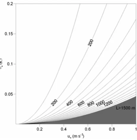
Fig. 1. BV behaviour for usual ranges of temperature and potential temperature gradient.

3 Theoretical considerations 3.1 BV calculation

This is the natural frequency of internal gravity waves or lee waves and may be calculated from

BV= g ∂2

∂z T

!1/2

, (1)

whereg is the acceleration due to gravity, 2the potential temperature andT the mean temperature between the two levels considered to calculate the potential temperature gra-dient. Since only temperatures were available, this gradient was obtained from

∂2 ∂z ≈

∂T

∂z +0, (2)

where0is the adiabatic lapse rate, which under dry condi-tions is 0.0098 K m−1_{. More stable stratification is}

associ-ated with higher values of this frequency, which cannot be defined in unstable conditions. BV is graphically depicted in Fig. 1 for usual ranges of temperature and potential tem-perature gradient. BV change with temtem-perature is about 8% in the temperature range considered and nearly independent from potential temperature gradient. Conversely, for a fixed temperature, changes in BV are more important (it increases some nine-fold in the potential temperature gradient range considered).

Figure 2.-

L

values for usual ranges of friction velocity and scale temperature.

Fig. 2.Lvalues for usual ranges of friction velocity and scale tem-perature.

3.2 L calculation

This is an atmospheric stability indicator which may be ob-tained from

L= T0u

2

∗

kgθ∗, (3)

whereu∗is the friction velocity (the square root of the kine-matic momentum flux),θ∗, the temperature scale (minus the kinematic heat flux divided by the friction velocity),T0, the

air temperature andk, von Karman’s constant, usually 0.4. Figure 2 presentsLas a function ofu∗andθ∗typical values. At lower temperature scale values, Lis extremely sensible to the friction velocity. However, Lis steadier against the temperature scale at higher values of this variable and lower friction velocity values.

Once wind speed and temperature profiles were known,L was iteratively determined by the similarity theory equations

U= u∗ k

ln

z z0

−ψm

z

L

+ψm

z₀

L

, (4)

2−20=

θ∗ k

ln

_z

z0

−ψh

z

L

+ψh

z₀

L

, (5)

whereUand2are wind speed and potential temperature at z,z0is the roughness length, 20, the potential temperature

at the roughness length andψm, andψhare experimentally determined similarity functions.

Assuming a neutral situation, i.e. logarithmic profiles, and a roughness length equal to 0.04 m, typical for long grass or

24

Figure 3.-

BV

profiles during day and night in the two most representative seasons of

the year. Average interquartile range was 0.015 s

during the night and 0.017 s

during

the day.

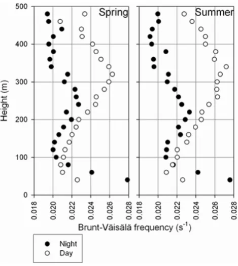
Fig. 3. BV profiles during day and night in the two most representa-tive seasons of the year. Average interquartile range was 0.015 s−1 during the night and 0.017 s−1during the day.

agricultural crops (Jacobson, 2005), a friction velocity equal to 1 m s−1implies a 19.56 m s−1wind speed at 100 m, which was a possible though infrequent value. A temperature scale equal to 0.1 K implies about a 2 K potential temperature dif-ference, which was much more frequent at night than during the day.

Since20was not known, Eq. (5) applied to 40 m was

sub-tracted from Eq. (5) applied to the z level, giving, 2−240=

θ∗ k

ln z 40

−ψh

z

L

+ψh

₄₀

L

. (6) Moreover, potential temperature differences on the left side of Eq. (6) were calculated from Eq. (2).

At the first step, wind speed and potential temperature profiles were considered logarithmic. With this assumption, similarity functions vanished and the firstL value was cal-culated from the first friction velocity and temperature scale values obtained by linear regression slopes where ln(z)was taken as the x-axis. PositiveLvalues are associated to stable atmosphere and negative values to unstable atmosphere.

In this paper, the following similarity functions were used (Arya, 2001):

ψm=ψh = −5z L, for

z L ≥0

ψm=ln

"

1+x2 2

!

1+x 2

2#

−2 tan−1x+π

2, (7)

for z L <0 ψh =2 ln

1+x2 2

!

, for z L <0 wherex= 1−15_Lz

1

4_{. With these functions, a newLvalue}

was obtained by linear regression from Eqs. (4), (6) by considering ln(z)–ψ(z/L) in the x-axis. Convergence was reached when two consecutiveLdiffered less than 1%.

4 Results

4.1 Boundary layer stratification from the BV

BV was calculated from temperature data for consecutive

lev-els and attributed to the lower level. The number of data was considerably greater below 200 m at night (taken from one hour before sunset to one hour after sunrise, following standard stability criteria). When seasonal daily and nightly medians were obtained, a stratified structure appeared par-ticularly in spring and summer, shown in Fig. 3, but also in autumn. From this figure, some remarks regarding BV behaviour with height may be made for both seasons. In general, frequencies lay in a narrow interval, from 0.018 to 0.028 s−1, according to values considered by Hyun et al. (2005), and stratification was more complex at night than during the day. During the night, the higher BV values were reached at the lowest level, 40 m, and a rapid decrease with height was noticeable up to around 100 m, where frequency was slightly above 0.020 s−1. From this level, frequency in-creased with height up to a maximum at 240 m in spring or 220 m in summer (both 0.023 s−1). Frequency then de-creased with height until nearly 340 m, where the value was about 0.020 s−1_{again. From this level, frequency remained}

almost constant with height. Consequently, a first layer was observed until about 100 m, a second until about 340 m and finally an upper third layer. Stability was highest at the low-est level, although there was another extremely stable layer at intermediate levels, around 200 m. During the day only two regions may be considered. With the exception of the first level, where the frequency was slightly above 0.022 s−1, the trend was increasing with height from about 0.021 s−1to a maximum at 320 m in spring (0.026 s−1)or 340 m in summer (0.027 s−1), at a similar rate (2×10−5s−1m−1). Frequencies at both maxima were the closest values to frequencies at 40 m during the night. Above these maxima, frequency decreased with height, more quickly in spring (4×10−5s−1m−1)than in summer (3×10−5s−1m−1). To sum up, during the day and with positive potential temperature gradients, stability was highest at about 300 m.

4.2 Stability classification

Equations (4), (6) were used with profiles from 40 to 100 m. This level was selected in order to retain surface layer

Table 1. Frequency of observations with first and thirdLquartiles for each class.

Class L(m) Frequency

First quartile Third quartile

Drainage 6760

Extremely stable 0.25 0.83 18 058

Stable 161.84 1299.49 14 044

Unstable −1436.50 −64.16 11 130

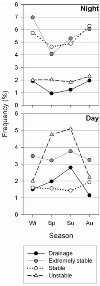
properties and to obtain sufficient data for regressions. How-ever, two special situations had to be considered. Firstly, slopes from Eq. (4) were sometimes negative, these pro-files being described as drainage. Secondly, the convergence criterion provided positiveLvalues without physical sense (L<1 m), these situations being referred to as extremely sta-ble. With these assumptions, a stability classification based on four classes was proposed with the following distribu-tion of observadistribu-tions: about 13% of profiles analysed cor-responded to drainage, 34% to extremely stable situations, 27% to other stable situations and 21% to unstable situations. The remaining profiles were discarded for reasons such as the low number of data (lower than 3) or high number of itera-tions (above 200). Table 1 shows frequencies observed for each class and their first and thirdLquartiles. This distribu-tion appeared correct since stability is the usual characteris-tic of the low atmosphere. Distribution of the profiles used is presented in Fig. 4 where the frequency contrast was sharper during the night. Higher frequencies in this period were as-sociated to extremely stable and stable situations, evidencing a seasonal pattern with lower values in spring and summer. However, both seasons showed the highest unstable frequen-cies during the day.

Since the calculation method was forward for stable and unstable situations, seasonal medians ofL, u∗ andθ∗ dur-ing day and night were obtained and presented in Fig. 5 to provide information on their quantity, yearly evolution and contrast amongst them. Yearly evolution was extremely soft, since the yearly pattern generally presented slightly lower values in spring and summer. L was nearly 500 m in sta-ble situations and showed a very slight contrast between day and night, 60 m, with lower values in the night, when stabil-ity was greater. For unstable situations,Lwas about−175 m during the day and 1200 m lower at night, revealing that this variable was less unstable in these conditions. Moreover, val-ues for stable situations might be considered moderate since they lay between those more extreme for unstable situations (considered without sign). u∗ was placed between 0.4 and 1 m s−1, proving particularly low during the day for stable situations in spring and summer. The only exception was for unstable situations during the night, whenu∗was

consid-Figure 4.- Seasonal distribution of profiles used.

Fig. 4. Seasonal distribution of profiles used.

erably higher, about 1.6 m s−1giving as a result the impor-tant values ofL. Although flux analysis is outside the scope of this paper, theseu∗high values revealed intense momen-tum fluxes. θ∗evidenced lower values for stable situations, 0.08 K on average, than for unstable situations, −0.30 K, when its value was noticeable during the day,−0.45 K, im-plying important heat fluxes. These highly negative values during the day were linked to the less negative values ofL.

In order to gain an insight into the classification suggested, a relationship with profiles was established by means of wind speed and temperature medians, which were calculated from 40 to 100 m for the four stability classes proposed and

26

Figure 5.- Seasonal medians of

L

,

u

and

θ

calculated during the day and night for

stable and unstable situations. Bars show the interquartile range.

Fig. 5. Seasonal medians ofL, u∗ andθ∗ calculated during the day and night for stable and unstable situations. Bars show the in-terquartile range.

presented in Fig. 6, which we will shortly comment on. The same scale was selected for all the plots in order to compare them, although some details, such as change with height, may be obscured.

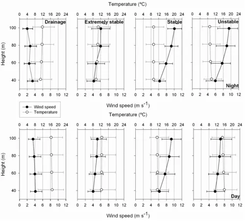
Drainage corresponded to very low winds (below 4.1 m s−1_{) decreasing with height, especially at night}

(1.4 m s−1_{until 100 m). Temperatures were highest, around}

11.4◦_{C during the night and 16.6}◦_{C during the day, and} tem-perature profiles were stable, mainly at night, when a 1◦C inversion was observed, whereas during the day temperature decreased with height.

Extremely stable situations considered low wind speed, but increasing with height (1.8 m s−1_{at night). Temperatures}

were moderate, 10.2◦C at night and 12.5◦C during the day. A noticeable inversion was observed at night (1.1◦C), whereas temperature was nearly constant with height during the day. Frequencies observed from Fig. 4 point to these profiles be-ing a specific local feature durbe-ing the day.

Stable situations were associated to the highest winds, slightly above 6 m s−1at 40 m, with a noticeable increasing with height, 3.8 m s−1 at night, but enveloped by the low-est temperatures, 9.3◦C at night and 11.3◦C during the day, which were nearly constant with height.

Finally, unstable situations evidenced similar wind speed profiles to stable situations during the night and flatter during the day, although temperature profiles were unstable, with temperature decreasing about 1◦C, i.e. considerably greater than the adiabatic lapse rate. The contrast in temperatures during day and night was the highest, 6◦C, since tempera-tures during the night were the second lowest, 9.4◦C, and during the day the second highest, 15.4◦C. Thermal stratifi-cation favoured vertical movements, explaining the intense momentum fluxes during the night when the wind gradient was high, whereas heat flux was noticeable during the day, when the wind speed gradient was low.

From this description several groupings may be estab-lished:

– As regards wind speed, two kinds may be considered.

On the one hand, drainage and extremely stable situa-tions, which evidenced a low wind speed, although a different slope in its profile, but similar temperature pro-files. On the other hand, stable and unstable situations displayed a higher wind speed with similar wind pro-files, but different temperature profiles.

– As regards wind profile slope, drainage must be

consid-ered separately from the other kinds where stability of temperature profiles decreased from extremely stable to unstable situations.

– As regards temperature profile stability, unstable

situa-tions must be separated from the remaining kinds where temperature profiles corresponded to stable stratifica-tion.

Figure 6.- Wind speed and temperature median profiles for the four stability classes

proposed during the day and night. Bars show the interquartile range.

Fig. 6. Wind speed and temperature median profiles for the four stability classes proposed during the day and night. Bars show the interquartile range.

4.3 CO2concentrations

CO2concentrations evidenced a 379.5 ppm median and were

lineally fitted, yielding an increase of 8 ppm over the whole measuring period. However, for our analysis purposes, they were detrended and their daily evolution was drawn by means of a box and whisker plot in Fig. 7. Each box represents the interquartile range where the median is repre-sented by a line. Whiskers extend from the 10th to the 90th percentiles and points correspond to the 5th and 95th per-centiles. Medians showed a noticeable daily pattern where concentrations increased during the night up to a maximum

of 4.29 ppm at 05:30 UTC, whereas they remained nearly constant during the day, between −5 and −6.7 ppm from 10:00 to 18:00 UTC, which may be explained by convective mixing and photosynthesis (Miyaoka et al., 2007). This daily pattern concurs with observations presented in the bibliog-raphy (Chen et al., 2007). Different factors, such as plant-soil activities, influenced daily behaviour. Since vegetation is not the main feature at the measurement site and Fig. 7 corresponds to the whole year, when including periods of very low plant-soil activities that were lasting, it seemed that the main factor responsible for this pattern was the bound-ary layer evolution. Consequently, the development of the

28

Figure 7.- Box plot showing the daily cycle of detrended CO

concentrations (from 1

August 2002 to 31 July 2005).

Fig. 7. Box plot showing the daily cycle of detrended CO2

concen-trations (from 1 August 2002 to 31 July 2005).

mixed layer was linked to lower concentrations, whereas the establishment of a ground surface temperature inversion de-termined the low dilution of concentrations. Moreover, in-version became more intense throughout the night and hence the highest values were recorded at the end of the night. 5th percentiles were steady (around−11 ppm with a highest dis-crepancy of 3.93 ppm), whereas 95th percentiles showed ex-tremely high values, between 30 and 40 ppm, from 00:00 to 06:00 UTC. Distributions were noticeably right skewed dur-ing the night and virtually symmetrical durdur-ing the day, when concentrations lay in a narrow interval, particularly from 13:00 to 15:30 UTC, this interval being around 14 ppm for 90% of observations.

4.4 Relationship between stability classes and CO2 con-centrations

CO2medians were calculated for the different stability

situ-ations and represented in Fig. 8. With regard to daily evolu-tion, a very soft cycle was observed for unstable and stable situations, whereas a sharp contrast between day and night appeared in extremely stable and drainage situations. When only the day is considered, concentrations were very sim-ilar for all stability situations in each season. However, a seasonal evolution was observed, with the highest concen-trations in winter, −3.40 ppm, and the lowest in summer, −8.39 ppm. As regards only night, great differences were observed. Under drainage conditions, CO2 concentrations

were considerably higher as compared to the other stabil-ity classes followed by extremely stable situations. In or-der to quantify these concentrations, nighttime medians were

29

Figure 8.- Half-hourly medians of CO2 concentrations calculated for the stability classes

proposed during the four seasons of the year (from 1 August 2002 to 31 July 2005).

Interquartile range was about 5 ppm during the day and similar to the higher

concentrations during the night.

Fig. 8. Half-hourly medians of CO₂concentrations calculated for the stability classes proposed during the four seasons of the year (from 1 August 2002 to 31 July 2005). Interquartile range was about 5 ppm during the day and similar to the higher concentrations during the night.

Figure 9.- Medians of

BV

and wind speed for stable situations during the night. Average

interquartile range was 0.016 s

for

BV

and 4.6 m s

for wind speed.

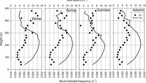
Fig. 9. Medians of BV and wind speed for stable situations during the night. Average interquartile range was 0.016 s−1for BV and 4.6 m s−1 for wind speed.

calculated and presented in Table 2. For all the stability cate-gories, higher CO2values corresponded to spring, especially

in drainage and extremely stable conditions, and lower val-ues to summer, mainly in stable and unstable situations. This behaviour seemed to be associated to the vegetation cycle. It is worth highlighting the highest median, 26.11 ppm, reached for drainage in spring, nearly 28 ppm higher than the median concentration in unstable conditions. As a final result, the main feature of the proposed stability classification was the ability to isolate high CO2concentrations and establish two

groups of concentrations, high and extremely high concen-trations, in situations with very low dilution.

4.5 Boundary layer structure

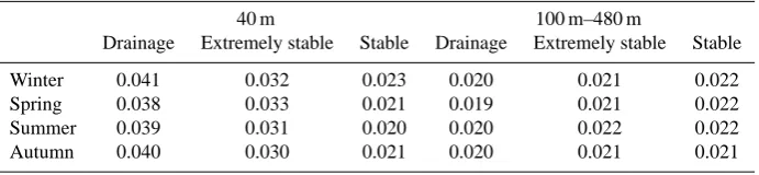
A relationship between BV and wind profiles based on sta-bility classes was considered. Firstly, Table 3 presents BV medians for 40 m and from 100 m to 480 m. This interval was chosen from the BV change observed at 100 m, since a fast decreasing with height was recorded below this level, whereas a nearly constant value was obtained above it. This table shows that drainage conditions were described by the highest BV at 40 m, around 0.039 s−1, but the lowest BV above 100 m, around 0.020 s−1, whereas stable conditions displayed the opposite behaviour, the lowest BV values at

Table 2. Seasonal medians of CO₂ concentrations (ppm) during the night for different stability conditions in the lower atmospheric boundary layer. Trend and mean value were removed.

Winter Spring Summer Autumn

Drainage 7.65 26.11 7.17 9.86

Extremely stable 2.91 11.73 −0.59 4.07

Stable −0.87 1.16 −7.25 −1.38

Unstable −1.83 −1.61 −9.37 −1.80

40 m, around 0.021 s−1, and the highest BV above 100 m, around 0.022 s−1. Extremely stable conditions evidenced frequencies between both cases.

Wind speed medians at 40 m for stable conditions were previously presented in Fig. 6, although when median wind speed profiles above 100 m were observed once median BV profiles were previously calculated, extremely stable situa-tions were associated to low level jets with cores near enough the surface for them to be assumed coupled to the surface (Mathieu et al., 2005) and wind speeds lower than 8 m s−1. In particular, a well defined low level jet was observed in summer, with a wind speed of 6.6 m s−1in the core at 120 m. However, the jets presented in Fig. 9 were quite different,

Table 3. Brunt-V¨ais¨al¨a frequency (s−1)medians during the night under different stability conditions.

40 m 100 m–480 m

Drainage Extremely stable Stable Drainage Extremely stable Stable

Winter 0.041 0.032 0.023 0.020 0.021 0.022

Spring 0.038 0.033 0.021 0.019 0.021 0.022

Summer 0.039 0.031 0.020 0.020 0.022 0.022

Autumn 0.040 0.030 0.021 0.020 0.021 0.021

since they were associated to stable situations with their cores below the higher BV. These were at around 220 m for winter and spring, with wind speeds around 12.5 m s−1. In summer, the core and wind speed were slightly lower, 200 m and around 11.5 m s−1_{. These features mean that the jets}

might be uncoupled from surface. The base of a well-defined low level jet in stable situations is associated to the height of the nocturnal boundary layer. Consequently, in extremely stable situations, this layer should be thinner and, extrapo-lating this result, drainage would be linked to the thinnest nocturnal boundary layer.

5 Conclusions

The boundary layer structure was analysed and a stability classification was established by means of BV andL calcu-lated with three years of RASS sodar and CO2observations

at a rural site.

BV revealed a stratified structure of the boundary layer,

especially in spring and summer. During the night, a highly stable layer was observed near the ground, where frequen-cies were near 0.028 s−1, although another stable layer was also seen from 100 to 340 m. During the day, frequencies increased with height, up to around 0.026 s−1at 320 m.

L was obtained by an original method involving linear regressions of wind speed and potential temperature differ-ences of the four lowest levels. Four stability classes were considered: drainage, extremely stable, stable (1≤L)and un-stable (L<0).

CO2detrended concentrations were considered, revealing

lower concentrations during the day and frequent high con-centrations at night.

Stability classes were related during the night to BV, wind speed and temperature profiles and CO2concentrations, with

the result that:

– Drainage was associated to very high frequencies

(around 0.039 s−1)at 40 m, although very low frequen-cies from 100 m (around 0.020 s−1), the lowest wind speed at 40 m (below 3.4 m s−1 that decreased with height), the highest temperatures with stable profiles be-low 100 m and very high CO2concentrations, mainly in

spring (26.11 ppm). These concentrations were asso-ciated to the very low dilution in a thin layer near the surface.

– Extremely stable situations were linked to intermediate

frequencies, low wind speed, moderate temperatures in the lower atmosphere, low levels jets coupled to sur-face, a 1.1◦C strong inversion below 100 m and the sec-ond highest concentrations, 11.73 ppm in spring. In this case, the layer where dilution occurred was con-sequently thicker than the layer associated to drainage.

– Stable situations were characterised by the lowest

fre-quencies at 40 m (around 0.020 s−1) and the highest from 100 m (around 0.022 s−1), the highest wind speed at 40 m (slightly higher than 6 m s−1) but the low-est temperature (9.3◦C), low level jets decoupled from surface with cores of about 12 m s−1 at 200 m below the higher BV and the second lowest concentrations, −7.25 ppm in summer.

– Unstable situations were associated to high wind speed,

superadiabatic temperature profiles below 100 m and the lowest concentrations,−9.37 ppm in summer.

Acknowledgements. The authors wish to acknowledge the financial support of the Interministerial Commission of Science and Technol-ogy and the Regional Government of Castile and Leon. The authors also acknowledge anonymous referees for their helpful comments, which have considerably improved the content of this paper.

Topical Editor F. D’Andrea thanks M. Kallistratova and another anonymous referee for their help in evaluating this paper.

References

Arya, S. P.: Introduction to Micrometeorology, second edition, Aca-demic Press, San Diego, California, 2001.

Augustin, P., Delbarre, H., Lohou, F., Campistron, B., Puygrenier, V., Cachier, H., and Lombardo, T.: Investigation of local mete-orological events and their relationship with ozone and aerosols during an ESCOMPTE photochemical episode, Ann. Geophys., 24, 2809–2822, 2006,

http://www.ann-geophys.net/24/2809/2006/.

Banta, R. M.: Stable-boundary-layer regimes from the perspective of the low-level jet, Acta Geophysica, 56, 58–87, 2008.

Bradley, S.: Atmospheric acoustic remote sensing, CRC Press, Boca Raton, Florida, 2008.

Chen, J. M., Chen, B., and Tans, P.: Deriving daily carbon fluxes from hourly CO2mixing ratios measured on the WLEF

tall tower: An upscaling methodology, J. Geophys. Res., 112, G01015, doi:10.1029/2006JG000280, 2007.

Cohen, L., Helmig, D., Neff, W. D., Grachev, A. A., and Fairall, C. W.: Boundary-layer dynamics and its influence on atmospheric chemistry at Summit, Greenland, Atmos. Environ., 41, 5044– 5060, 2007.

Cvitan, L.: Classification of the stratified atmospheric boundary layers at Molve (Croatia) based on the similarity theory, Mete-orol. Atmos. Phys., 93, 235–246, 2006.

De Bruin, H. A. R., Ronda, R. J., and Vandewiel, B. J. H.: Approx-imate solutions for the Obukhov length and the surface fluxes in terms of bulk Richardson numbers, Bound.-Lay. Meteorol., 95, 145–157, 2000.

Elansky, N. F., Lokoshchenko, M. A., Belikov, I. B., Skorokhod, A. I., and Shumskii, R. A.: Variability of trace gases in the atmo-spheric surface layer from observations in the city of Moscow, Izv. Atmos. Ocean. Phys., 43, 219–231, 2007.

Emeis, S., Jahn, C., M¨unkel, C., M¨unsterer, C., and Sch¨afer, K.: Multiple atmospheric layering and mixing-layer height in the Inn valley observed by remote sensing, Meteorol. Z., 16, 415–424, 2007.

Emeis, S. and Sch¨afer, K.: Remote sensing methods to investi-gate boundary-layer structures relevant to air pollution in cities, Bound.-Lay. Meteorol., 121, 377–385, 2006.

Engelbart, D. A. M., Kallistratova, M., and Kouznetsov, R.: Deter-mination of the turbulent fluxes of heat and momentum in the ABL by ground-based remote-sensing techniques (a Review), Meteorol. Z., 16, 325–335, 2007.

Esau, I. N. and Zilitinkevich, S. S.: Universal dependences between turbulent and mean flow parameters instably and neutrally strat-ified Planetary Boundary Layers, Nonlin. Processes Geophys., 13, 135–144, 2006,

http://www.nonlin-processes-geophys.net/13/135/2006/. Foken, T.: 50 years of the Monin-Obukhov similarity theory,

Bound.-Lay. Meteorol., 119, 431–447, 2006.

Frech, M.: A simple method to estimate the eddy dissipation rate from SODAR/RASS measurements, 16th Symp. Bound. Layer and Turbulence, 9–13 August 2004, Portland, ME, USA, art. 6.13, 2002.

Garc´ıa, M. A., S´anchez, M. L., P´erez, I. A., and de Torre, B.: Con-tinuous carbon dioxide measurements in a rural area in the up-per Spanish plateau, J. Air Waste Manage. Assoc., 58, 940–946, 2008.

Gariazzo, C., Papaleo, V., and Pelliccioni, A.: Statistical compar-ison of modelled and SODAR measured turbulence data in a coastal area, Meteorol. Z., 16, 383–392, 2007.

Gariazzo, C., Pelliccioni, A., Di Filippo, P., Sallusti, F., and Ceci-nado, A.: Monitoring and analysis of volatile organic compounds around an oil refinery, Water Air Soil Pollut., 167, 17–38, 2005.

Grechko, Y. I., Rakitin, V. S., Fokeeva, Y. V., Dzhola, A. V., Pekur M. S., and Time, N. S.: Study of the effect of atmospheric bound-ary layer on carbon monoxide content variability at the center of Moscow, Izv. Atmos. Ocean. Phys., 29, 6–13, 1993.

Grisogono, B., Kraljevi´c, L., and Jeriˇcevi´c, A.: The low-level kata-batic jet height versus the Monin-Obukhov height, Q. J. Roy. Me-teorol. Soc., 133, 2133–2136, 2007.

Ha, K. J., Hyun, Y. K., Oh, H. M., Kim, K. E., and Mahrt, L.: Eval-uation of boundary layer similarity theory for stable conditions in CASES-99, Mon. Weather Rev., 135, 3474–3483, 2007. Hyun, Y. K., Kim, K. E., and Ha, K. J.: A comparison of methods

to estimate the height of stable boundary layer over a temperate grassland, Agric. For. Meteorol., 132, 132–142, 2005.

Jacobson, M. Z.: Fundamentals of Atmospheric Modeling, second edition. Cambridge University Press, Cambridge, 2005. Kallistratova, M. A. and Coulter, R. L.: Application of SODARs in

the study and monitoring of the environment, Meteorol. Atmos. Phys., 85, 21–37, 2004.

Karipot, A., Leclerc, M. Y., Zhang, G., Martin, T., Starr, G., Hollinger, D., McCaughey, J. H., and Hendrey, G. R.: Nocturnal CO2exchange over a tall forest canopy associated with

intermit-tent low-level jet activity, Theor. Appl. Climatol., 85, 243–248, 2006.

Kopeykin, V. M., Kapustin, V. N., and Pekur, M. S.: Monitoring of soot aerosol in the atmosphere of Moscow, Izv. Atmos. Ocean. Phys., 29, 198–202, 1993.

Mathieu, N., Strachan, I. B., Leclerc, M. Y., Karipot, A., and Pattey, E.: Role of low-level jets and boundary-layer properties on the NBL budget technique, Agric. For. Meteorol., 135, 35–43, 2005. Miyaoka, Y., Inoue, H. Y., Sawa, Y., Matsueda, H., and Taguchi, S.: Diurnal and seasonal variations in atmospheric CO2in Sapporo,

Japan: Anthropogenic sources and biogenic sinks, Geochem. J., 41, 429–436, 2007.

Pekour, M. S. and Kallistratova, M. A.: Sodar study of the boundary layer over Moscow for air pollution application, Appl. Phys. B, 57, 49–55, 1993.

Pernigotti, D., Rossa, A. M., Ferrario, M. E., Sansone, M., and Benassi, A.: Influence of ABL stability on the diurnal cycle of PM10 concentration: illustration of the potential of the new

Veneto network of MW-radiometers and SODAR, Meteorol. Z., 16, 505–511, 2007.

Smedman, A. S., H¨ogstr¨om, U., Huntb, J. C. R., and Sahl´ee, E.: Heat/mass transfer in the slightly unstable atmospheric surface layer, Q. J. Roy. Meteorol. Soc., 133, 37–51, 2007.

Sorbjan, Z.: An examination of local similarity theory in the sta-bly stratified boundary layer, Bound.-Lay. Meteorol., 38, 63–71, 1987.

Zilitinkevich, S. S. and Esau, I. N.: Similarity theory and calcu-lation of turbulent fluxes at the surface for the stably stratified atmospheric boundary layer, Bound.-Lay. Meteorol., 125, 193– 205, 2007.