www.ann-geophys.net/26/259/2008/ © European Geosciences Union 2008
Annales
Geophysicae
Predicting cycle 24 using various dynamo-based tools
M. Dikpati
High Altitude Observatory, National Center for Atmospheric Research, Boulder, CO, USA
Received: 12 February 2007 – Revised: 16 May 2007 – Accepted: 5 June 2007 – Published: 26 February 2008
Abstract. Various dynamo-based techniques have been used to predict the mean solar cycle features, namely the ampli-tude and the timings of onset and peak. All methods use information from previous cycles, including particularly po-lar fields, drift-speed of the sunspot zone to the equator, and remnant magnetic flux from the decay of active regions. Po-lar fields predict a low cycle 24, while spot zone migration and remnant flux both lead to predictions of a high cycle 24. These methods both predict delayed onset for cycle 24. We will describe how each of these methods relates to dynamo processes. We will present the latest results from our flux-transport dynamo, including some sensitivity tests and how our model relates to polar fields and spot zone drift methods.
Keywords. Solar physics, astrophysics,and astronomy (Magnetic fields; Stellar interiors and dynamo theory; Instruments and techniques)
1 Introduction
Understanding the mechanism of the solar activity cycle and predicting the the upcoming cycles’ features remain a key area of research in solar physics and space science. The so-lar activity cycle influences the terrestrial systems in vari-ous ways: posing hazards to satellites, disrupting powergrids, causing blackouts in radio and telecommunication systems, even affecting the astronauts in space.
An oscillatory magnetohydrodynamic dynamo, operating somewhere inside the Sun, is most likely responsible for pro-ducing a solar cycle. Physical basis of a solar cycle pre-diction tool should be intimately associated with the under-standing of solar dynamo processes. In this talk, we will Correspondence to: M. Dikpati
present a review of various attempts for building dynamo-based schemes for predicting solar cycles and their step-by-step successes. We close by commenting on what should be the future goals in this topic of research.
2 The dynamo-based tools
Predicting the properties of an upcoming solar cycle started about 40 years ago. The methods were purely statistical in those early days. The attempt to find the physical foundation of a solar cycle prediction scheme was first made in 1970s in a conceptual qualitative way by Schatten et al. (1978) who postulated a magnetic persistence between the amplitude of the current sunspot cycle and the previous cycle’s polar field after the reversal. In this scheme, a Babcock-Leighton dy-namo was considered; the polar fields arise from the decay of the following-polarity spot of a tilted, bipolar active re-gion, and then these large-scale dipolar poloidal fields were assumed to be wrapped up by the pole-to-equator differen-tial rotation (see the schematic diagram in Fig. 1 of Schatten, 2002) to generate the spot-producing toroidal fields. There-fore, in this conception it is the latitudinal fields that are being sheared by the Sun’s latitudinal differential rotation. Hence the derivation of latitudinal fields from the radial polar fields is necessary to make a quantitative prediction of cycle ampli-tude.
Schatten’s important first attempt led us to investigate the physics behind the following two issues: (i) if the polar fields from the previous cycle determine the amplitude of the next cycle, how are such polar fields transported to the shear-layer at the bottom in 5.5 years? (ii) Do they remain radial down to the shear-layer? (iii) Are the stronger radial fields associated with stronger, or weaker latitudinal fields?
260 M. Dikpati: Dynamo-based prediction tools
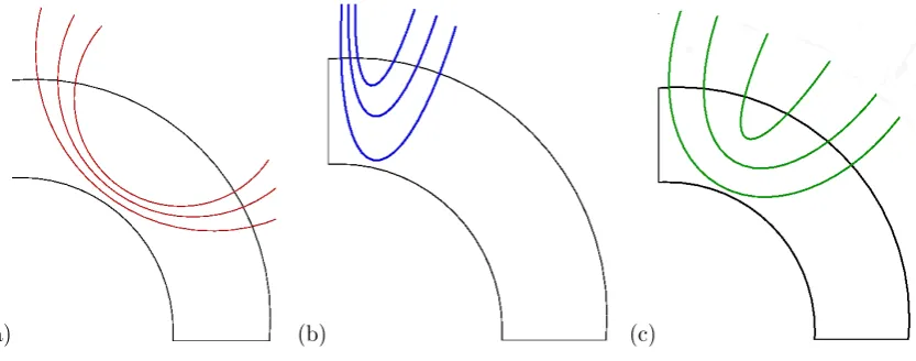
[image:2.595.92.509.65.229.2](a) (b) (c)
Fig. 1. Depending on the field geometry below the surface, (a) weak radial fields could be associated with strong latitudinal fields or (b) vice
versa, or weak radial fields could also be associated with weak latitudinal fields (c).
major processes that can transport the large-scale magnetic fields from the surface to the bottom of the convection zone, namely turbulent diffusion and advection by meridional cir-culation. Although observations give some measurements about the amplitudes of the diffusivity and the meridional flow speed near the surface, but very little is known about the profiles and amplitudes of these processes in the deeper layers below the surface. Therefore theoretical knowledge about the transport processes are currently the best possible options that can help determine how long the surface polar fields would take to reach the bottom of the convection zone. Figure 1 below demonstrates how the weak polar fields could give rise to strong or weak latitudinal fields depending on the field geometry below the surface. Unless the surface polar fields reach the bottom in just 5.5 years and unless the latitudinal fields associated with those radial fields are posi-tively correlated, the spot-producing toroidal fields at the bot-tom cannot be positively correlated with the previous cycle’s polar fields. Nonetheless, predictions about upcoming cy-cles have been made using this scheme (also called the “polar field precursor method”) which forecasts a very weak cycle 24 (Schatten, 2005; Svalgaard et al., 2005).
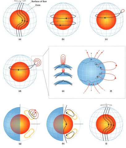
Very recently the quantitative estimation of upcoming cy-cle’s spot-producing flux by directly integrating the induc-tion equainduc-tions forward in time has begun and is rapidly gain-ing interest (Dikpati et al., 2006; Dikpati and Gilman, 2006; Cameron and Sch¨ussler, 2007). These models assimilate the observed magnetic data from the surface. Data assimilation techniques have been used in atmospheric weather prediction models since 1950s. It is starting now in solar cycle models. The reason is that a particular class of solar cycle models, namely the flux-transport dynamos, is calibratible to the Sun. Figure 2 describes how a flux-transport dynamo works. Basically it involves the following processes: (i) shearing of a pre-existing poloidal fields by the Sun’s differential
rota-tion to produce new toroidal fields, followed by eruprota-tions of sunspots (shown in panels a, b, c of Fig. 2), (ii) spot-decay and flux-spreading to produce new global poloidal fields at the surface (panels e, f, g) and (iii) transport of poloidal fields by the meridional circulation conveyor belt toward the pole and down to the bottom of the convection zone, followed by regeneration of new toroidal fields of opposite sign. The physical foundation of the “magnetic persistence” effect, or the duration of the Sun’s memorry of its past magnetic fields, can be understood in this class of dynamos with the help of Fig. 2 which demonstrates that a mass-conserving meridional flow with a solar-like surface flow-speed would take about 20 years to carry the poloidal magnetic flux from the mid-latitude at the surface to the mid-mid-latitude at the bottom of the convection zone. Therefore, the Sun’s poloidal fields from a few past cycles, rather than just the previous cycle’s po-lar fields, should contribute in determining the “seed” for the next cycle’s spot-producing fields.
Fig. 2. Schematic of solar flux-transport dynamo processes. Red inner sphere represents the Sun’s radiative core and blue mesh the solar
surface. In between is the solar convection zone where dynamo resides. (a) Shearing of poloidal field by the Sun’s differential rotation near convection zone bottom. The Sun rotates faster at the equator than the pole. (b) Toroidal field produced due to this shearing by differential rotation. (c) When toroidal field is strong enough, buoyant loops rise to the surface, twisting as they rise due to rotational influence. Sunspots (two black dots) are formed from these loops. (d, e, f) Additional flux emerges (d, e) and spreads (f) in latitude and longitude from decaying spots (as described in Fig. 5 of Babcock, 1961). (g) Meridional flow (yellow circulation with arrows) carries surface magnetic flux poleward, causing polar fields to reverse. (h) Some of this flux is then transported downward to the bottom and towards the equator. These poloidal fields have sign opposite to those at the beginning of the sequence, in frame (a). (i) This reversed poloidal flux is then sheared again near the bottom by the differential rotation to produce the new toroidal field opposite in sign to that shown in (b).
predicted to be delayed by 12 months in the former case (see the blue curve in Fig. 3a) and by 6 months in the latter case (green curve in Fig. 3a) with respect to an average 10.5 year
262 M. Dikpati: Dynamo-based prediction tools We note here that by “onset of a new cycle” we do not
mean the appearance of the “first” new cycle’s spot, rather the time when the flux from new cycle’s spots exceeds the flux from old cycle’s spots. Predicting the “first” new cycle’s spot is not yet possible from such flux-transport models, be-cause the spot eruption process is not directly included in such models; instead, the models assume that the tachocline toroidal flux buoyantly erupted at the surface, when it ex-ceeds a certain field strength, is the proxy for the spot-flux.
The first truly dynamo-based simulation of the sequence of peaks of past solar cycles and a forecast of solar cycle 24 was published by Dikpati and colleagues (Dikpati et al., 2006; Dikpati and Gilman, 2006). These simulations and forecast were done by starting from the calibrated flux transport dy-namo of Dikpati et al. (2004) and making certain modifica-tions. First, in their Eq. (3) for the poloidal field in terms of vector potentialA, the link between the toroidal field in the dynamo at the bottom and the poloidal field at the surface is replaced by a surface forcing term that is derived from the waxing and waning of the observed poloidal fields created by the decay of tilted bipolar active regions in previous so-lar cycles. This represents a form of 2-D (time-latitude) data assimilation in the model, a very common practice for me-teorological forecast models, but perhaps the first time it has been used in a solar forecasting problem.
As a result of the above modification, no quenching of the Babcock-Leighton poloidal source and no buoyancy mecha-nism are included in the model. Mathematically, the model is changed from being a self-contained nonlinear system (the only nonlinearity being in the quenching of theα-effects) to a truly linear system that is forced at the upper boundary by a measure of the sun’s past surface fields. The resulting equa-tion forAis given by
∂A
∂t + 1
rsinθ(u.∇)(rsinθ A)= η
∇2− 1
r2sin2θ
A+F(r, θ, t )+αBφ, (1)
in which all variables and parameters are measured in c.g.s. units. The meridional flow (u=ureˆr+uθeˆθ) has the following
form: ur(r, θ )=u0
R
r
2
− 1
m+1 + c1
2m+1ξ
m
− c2
2m+p+1ξ
m+p
ξsinqθ[(q+2)cos2θ−sin2θ], (2a)
uθ(r, θ )=u0
R
r
3
−1+c1ξm−c2ξm+p
×sinq+1θ cosθ, (2b)
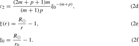
in which, c1=
(2m+1)(m+p) (m+1)p ξ0
−m, (2c)
c2=
(2m+p+1)m (m+1)p ξ0
−(m+p), (2d)
ξ(r)=R
r −1, (2e)
ξ0=
R
r0
−1. (2f)
Here m=1.5 is the exponent for an adiabatically strat-ified solar convection zone with a density profile ρ(r)=ρb
(R/r)−1 m
(ρb denotes the density at the
convection zone base). The other two parameters have valuesp=1.0 andq=2.0.
The surface forcing function,F, is derived from the ob-servational data in such a way as to capture the time-varying production of poloidal fields from the decay of active re-gions. The construction of this forcing could be done in a variety of ways; here we represent it with a Gaussian profile of fixed width, migrating towards the equator at a fixed rate, but with a peak determined by the amplitude of smoothed sunspot area data.
This surface forcing function imposes on the model the (variable) period of past solar cycles. But as described above and in Dikpati and Charbonneau (1999), flux-transport dy-namos already have their own intrinsic period, determined primarily by the strength of the meridional flow. We do not know directly from velocity observations prior to 1996 what the amplitude of this meridional flow was. The best we can do is to estimate an average amplitude of meridional flow from the average period of as many past cycles as we have high quality sunspot data for, which takes us back to cycle 12. From this data we get an average period of 10.75 years.
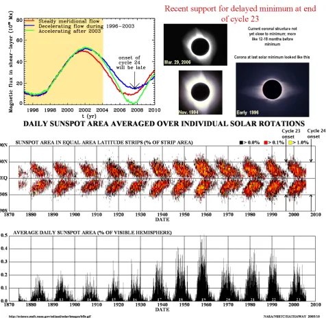
[image:4.595.308.546.58.138.2]If we use a meridional flow amplitude determined in this way, but force the model with data that has the observed pe-riod of each sunspot cycle, a phase mismatch in the link be-tween the toroidal and poloidal fields grows to an unaccept-ably large value over several cycles’ time integration. This makes simulation and forecast of cycle peaks impossible. To avoid this problem, Dikpati deToma and Gilman stretched and compressed in time the observed data so that each cycle in the surface forcing had the same period, 10.75 years, as the intrinsic period of the dynamo, so that no such destruc-tive phase mismatches would occur. As a result, this method cannot be used to simulate or predict the period of an up-coming cycle, but it can be used to predict the amplitude. Figure 4a compares the stretched and compressed sunspot data with the original data. Then we represent the latitude distribution of the poloidal source within each cycle by a Gaussian with half-width 6◦latitude (Fig. 4b) whose peak
Fig. 3. (a) Time trace of integrated toroidal flux in bottom shear layer for simulations beginning in 1995 with 3 different meridional flow
variations with time; (b) Coronal images at eclipse, showing 2006 corona not at minimum phase (c) observed butterfly diagram from David Hathaway’s website.
Strictly speaking, the surface poloidal forcing should come from synoptic observations of the photospheric mag-netic flux that originates from the decay of active regions, but such measurements exist only from 1976. But photo-spheric magnetic flux and sunspot area averaged over several rotations correlate very well with a linear fit (Dikpati et al., 2006), so we are able to use the much longer sunspot area record to create the forcing.
Starting from a fully converged calibrated model solution, we initialized the model from the beginning of solar cycle 12, and ran it for the next 13 cycles extending through the up-coming cycle 24. The time step of this calculation was 0.25 days, determined by CFL condition.
[image:5.595.60.537.59.526.2]264 M. Dikpati: Dynamo-based prediction tools
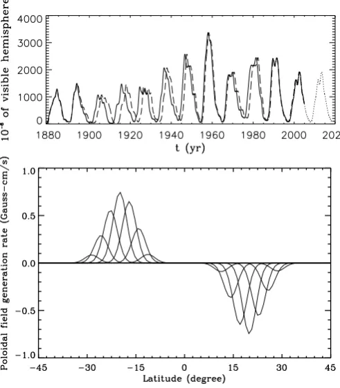
Fig. 4. (a) sunspot area data stretched and compressed (dashed
curve) in time to equalize all solar cycle periods to 10.75 years, compared to original data (solid curve); (b) Gaussian profiles used to represent latitude width of sunspot zone at various phases of a sunspot cycle.
to 10.75 years) with the sequence of simulated peaks. It is clear from Fig. 5a that the correspondence between observed and simulated cycles is very good, particularly beyond cycle 15. For the first few cycles the agreement is not as good, because the model is still loading the meridional circulation “conveyer belt” with fields from previous cycles. The sim-ulations show two curves for the upcoming cycle 24. The solid curve represents the case for which the meridional cir-culation remains fixed at a value that produces the 10.75 year dynamo period, and shows cycle 24 should have a∼50% higher peak than cycle 23. The dashed curve represents a simulation that takes account of time variations in observed meridional circulation since 1996. For this case, cycle 24 is forecast to be∼30% higher than cycle 23. Thus, even allow-ing for variations in meridional circulation, we forecast that cycle 24 will be substantially more active than the current cy-cle. There are many other forecasts for cycle 24, most saying it will be larger than 23, but some saying it will be smaller. But our forecast is the very first one made using a dynamo model with real solar data.
The skill of our forecast model is demonstrated more clearly in the scatterplot shown in Fig. 5c. There
plot-Fig. 5. (a) Observed sunspot area data for cycles 12–23; (b) integral
from 0−45◦latitude of simulated toroidal magnetic flux in bottom shear layer for cycles 12–24, plus two forecasts for cycle 24; (c) scatterplot of sunspot area peaks vs peak of toroidal magnetic flux integral.
ted are the observed peaks for cycles 12–23 from Fig. 5a, against the peaks of the toroidal flux integral computed for the tachocline between the equator and 45◦, from Fig. 5b.
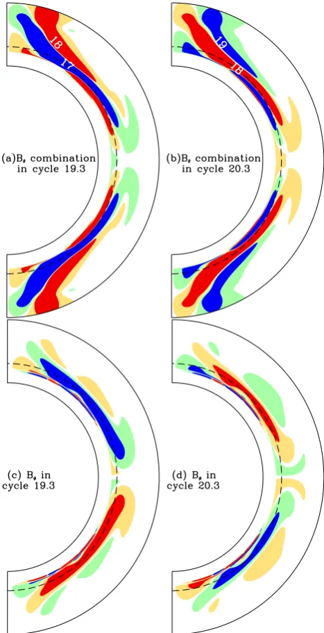
[image:6.595.47.293.66.347.2] [image:6.595.313.542.66.495.2]How the model works to achieve its forecast skill is dis-cussed in detail in Dikpati and Gilman (2006). A key element of its workings is shown in Fig. 6, in which is plotted the lat-itudinal poloidal field and the toroidal field at similar phases in cycles 19 and 20. The frames in Fig. 6 are snapshots from a continuous video animation for cycles 16–23, in which the path followed by new poloidal field of a particular sign in Bθ can be tracked until it disappears near the base of the
convection zone near the equator 2–3 cycles later. The num-bers within the plot denote the cycle of origin of each field tracked in this way through all of cycles 16–23. Figure 6 shows an example illustrating the memory of the model’s poloidal fields from previous cycles, with up to 3 successive cycles’ fields accumulated at high latitudes by the meridional flow. The latitudinal differential rotation shearing these fields produces the toroidal fields shown. The equatorward-flowing bottom branch of the meridional circulation then sweeps both poloidal and toroidal fields toward the equator to put in place the toroidal field that creates the peak of the next cycle. In this example, the maximum flow speed was 14.5 m s−1and the convection zone diffusivity 5×1010cm2s−1. The length of memory is determined by the relative amplitudes of the magnetic diffusivity and the meridional flow. For weaker meridional flow and/or higher magnetic diffusivity than the example shown, the memory would be shorter than three cycles, down to 1 cycle for 2×1011cm2s−1in the bulk of convention zone. For lower diffusivity and stronger flow the memory of the model gets longer.
We close this section with discussion of a very recent predictive flux-transport model by Cameron and Sch¨ussler (2007). They postulated that the cross-equatorial transport of magnetic flux in the late phase of a cycle is a accurate pre-cursor for the strength of the next cycle. They assimilated observed surface magnetic data into their one-dimensional surface flux-transport model, integrated it forward in time to estimate that transport, and predicted the next cycle’s ampli-tude. They find a very high correlation (r=0.90) between the observed amplitude of the next cycle and their predicted cross-equatorial transport at the end of the previous cycle, when they represent the latitude information of the surface poloidal source with equatorward migrating Gaussian as in Dikpati and Gilman (2006). They also predict high cycle 24. By contrast, the polar field predicted from the same model correlates poorly with the amplitude of the next cycle (see Fig. 1 of Cameron and Sch¨ussler, 2007). This result casts doubt on the utility of the so-called polar field precursor tech-niques.
However, assimilating the observed daily latitude profile of the emerged flux into the model integration, Cameron and Sch¨ussler (2007) find that the correlation between the cross-equatorial magnetic flux transport and the amplitude of the next cycle declines to a correlation coefficient of only 0.45. They also demonstrated by performing 1000 experi-ments with random sequences of eight previous cycles that the next cycle can be predicted with a median correlation
co-Fig. 6. (a), (b) latitudinal component of simulated poloidal field
(red and blue opposite signs) at phase 0.3 of cycles 19 and 20; (c),
(d) same for simulated toroidal field.
efficient ofr=0.83, only if the timing of the minimum before the cycle to be predicted is precisely known.
[image:7.595.309.543.63.519.2]266 M. Dikpati: Dynamo-based prediction tools the same as in Dikpati and Gilman (2006) if we correlate
the model output with the long-term averaged spot area data. This is because our model with high surface diffusivity and long traversal time for the surface flux to reach the bottom, smoothes out the short-term fluctuations.
3 The geomagnetic indices
Feynman (1982) first developed a tool based on the so-called aageomagnetic index. She showed to how to split this index intoaaT, a component that is in-phase with solar cycle and
can be related to the toroidal field (the spot-producing field) of the Sun, and aaaP, index that is out-of-phase with the
so-lar cycle, and can be related to the Sun’s poloidal fields. The aaP was shown to be a good precursor for predicting the
am-plitude of the next solar cycle. Very recently Hathaway and Wilson (2006) used this method to predict a high solar cycle 24. This result is consistent with their prediction obtained from the correlation of the latitudinal drift speed of centroid of sunspot zone and the second following cycle (Hathaway and Wilson 2004). This correlation is also consistent with the “time-delay” or the “magnetic persistence” effect in flux-transport type dynamos.
4 Issues regarding dynamo-based prediction tools
Certain criticisms have been put forward concerning fore-casting solar cycle peaks using a flux-transport dynamo model (Tobias et al., 2006). We were not allowed by Nature editors to respond to it, so we respond here and elsewhere.
The authors of this letter state a priori that because they contain parameterizations, flux-transport dynamos have no predictive power. But it is a logical certainty that predictive skill of ALL models, not just flux transport dynamos, can only be judged a posteriori by the results they produce. Fur-thermore the skill of our model cannot be tested by using some other model with other physics, such as one that omits meridional circulation and the time-latitude data assimila-tion. Also, much of the uncertainty of the effect of poorly known parameterizations of physical processes is in effect removed by calibrating the model to solar observations, and then forecasting only departures from the calibrated solu-tions. This is common practice and used with great success in forecast models in other fields, such as meteorology.
Tobias et al. also claim that since the dynamo equations are extremely nonlinear, chaos intrinsic to the system makes prediction much more difficult, particularly for longer time periods. Within a solar cycle, there are short-term chaotic features which are probably governed by a variety of nonlin-ear processes including the buoyant rise of initially toroidal fluxtubes. But we are not attempting to forecast them with our forced linear predictive tool. Obviously there are aggre-gate effects of many short-term nonlinear events which lead to, for example, the average surface poloidal fields that have
a well-defined observed pattern. Our predictive tool captures this pattern. By analogy, mean flow in a river can be forecast without forecasting accurately the various eddies that occur in the flow.
5 Discussion and conclusions
We have shown above that flux-transport dynamos when ap-plied to the sun can answer many important questions, from what determines the dynamo period to how the fields of pre-vious cycles determine the amplitude of the next one. Build-ing on this success, we plan many sensitivity tests of the model, and expect to generalize it to ultimately forecast both the period and the amplitude, as well as simulate and even forecast the appearance and evolution of nonaxisymmetric features, such as active longitudes. We already know that when we split the observed surface magnetic data into North-ern and SouthNorth-ern Hemispheres, we are able to correctly sim-ulate the large differences in amplitude between hemispheres in later cycles when they occur.
Acknowledgements. We thank P. Gilman for a thorough review of
the manuscript and for his helpful comments. This work is par-tially supported by NASA grants NNH05AB521, NNH06AD51I and the NCAR Director’s opportunity fund. National Center for Atmospheric Research is sponsored by the National Science Foun-dation.
Topical Editor R. Forsyth thanks R. Cameron and another anonymous referee for their help in evaluating this paper.
References
Cameron, R. and Sch¨ussler, M.: Solar cycle prediction using precur-sors and flux transport models, The Astrophys. J., 659, 801–811, 2007.
Dikpati, M.: Global MHD Theory of Tachocline and the Current Status of Large-Scale Solar Dynamo, in: Proceedings of the SOHO 14/GONG 2004 Workshop on “Helio- and Asteroseis-mology: Towards a Golden Future”, edited by: Danesy, D., ESA-SP, 559, 233–240, 2004.
Dikpati, M. and Charbonneau, P.: A Babcock-Leighton Flux Trans-port Dynamo with Solar-like Differential Rotation, The Astro-phys. J., 518, 508–520, 1999.
Dikpati, M., de Toma, G., and Gilman, P. A.: Predicting the strength of solar cycle 24 using a flux-transport dynamo-based tool, Geo-phys. Res. Lett., 33, L05102, doi:10.1029/2005GL024971, 2006. Dikpati, M. and Gilman, P. A.: Simulating and Predicting Solar Cycles Using a Flux-Transport Dynamo, The Astrophys. J., 649, 498–514, 2006.
Feynman, J.: Geomagnetic and solar wind cycles, 1900–1975, J. Geophys. Res., 87, 6153–6162, 1982.
Hathaway, D. H. and Wilson, R. M.: What the Sunspot Record Tells Us About Space Climate, Sol. Phys., 224, 5–19, 2004.
Schatten, K.: Fair space weather for solar cycle 24, Geophys. Res. Lett., 32, L21106, doi:10.1029/2005GL024363, 2005.
Schatten, K.: Solar activity prediction: Timing predictors and cycle 24, J. Geophys. Res., 107, SSH 15 1–7, 2002.
Schatten, K., Scherrer, P. H., Svalgaard, L., and Wilcox, J. M.: Us-ing dynamo theory to predict the sunspot number durUs-ing solar cycle 21, Geophys. Res. Lett., 5, 411–414, 1978.
Svalgaard, L., Cliver, E. W., and Kamide, Y.: Sunspot cycle 24: Smallest cycle in 100 years?, Geophys. Res. Lett., 32, L01104– L01107, doi:10.1029/2005GL024363, 2005.