BREAK-EVEN ANALYSIS
This chapter covers the basics of break-even analysis, the simplest analytical tool in management. It details what break-even analysis is, what it is used for, what definitions are used in break-even analysis and how break-even analysis can be helpful in decision-making of professionals in construction industry.
In construction industry, break-even analysis can be a handy tool to find answers to questions such as: How many years should I operate the facility to recover the initial investment and annual operating costs? How much does our company need to sell to reach the desired profitability? What should be the toll rate to cover my costs?
Break-even analysis for a single project
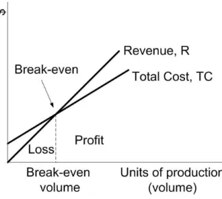
Definitions: Basically, break-even analysis determines the “break-even point”, at which operations neither make money nor loose money (Paek 2000, Blank and Tarquin 2008). At the break-even point, there is no gain or loss; hence costs or expenses are equal to revenues/incomes.
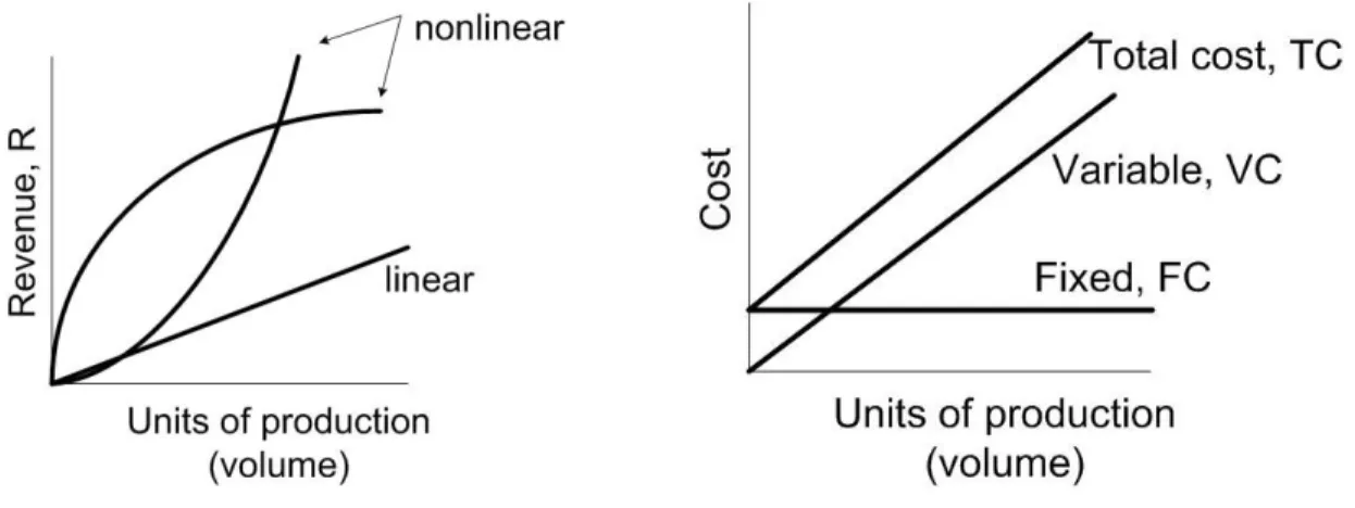
Break-even analysis utilizes two types of inputs for calculation of costs as: fixed costs and variable costs:
Fixed cost represents the expenses that are not related with the volume of production (or activity level) over a feasible range of operations. Examples include buildings, insurance expenses, depreciation, overheads, cost of information systems (Blank and Tarquin 2008). It is the sum of all costs to produce the first unit of a product. Another example could be the cost of an excavation equipment regardless of the excavation work performed on different projects.
Total cost is the sum of the fixed and total variable costs for any production or construction. Total revenue is the product of expected unit sales and the unit price of each unit.
Cost/expense and revenue/income relations are commonly assumed as linear; however non-linear relations are more realistic with more revenue for larger volumes (Blank and Tarquin 2008). Examples of different revenue cost relations are presented in Figure 1.
(a) Revenue relations – linear, increasing and decreasing per unit of production
(b) Linear cost relations
Figure 1. Linear and nonlinear revenue cost relations (copyright © Blank and Tarquin 2008).
Mathematically, the formula for break-even point can be shown as:
where;
TR represents the total revenues and TC represents total costs or expenses for an operation.
TR = TC
or
Here, Q (expected unit sales) is break-even point in sales. As seen from the above formulation, break-even analysis depends on fixed costs, variable costs, unit price of a product and expected unit sales (volume of sales). Graphical depiction of break-even point is provided in Figure 2.
Figure 2. Graphical depiction of break-even point (copyright © Blank and Tarquin 2008).
Example: Assume that as an investor, you are planning to enter the construction industry as a panel formwork supplier. Given the size of the construction industry in Turkey and the potential number of forthcoming projects, you forecasted that within two years, your fixed cost for producing formworks is $ 300 000. The variable unit cost for making one panel is $ 15. The sale price for each panel will be $ 25. If you charge $ 25 for each panel, how many panels you need to sell in total, in order to start making money?
TR = TC
Expected unit sales (Q) x Unit price (P) = Fixed cost (FC) + Total variable cost (VC)
Q x P = FC +Variable unit cost (V) x Expected unit sales(Q) QxP = FC + (VxQ)
Solution:
Variable unit cost = $ 15/panel Total fixed cost =$ 300 000 Price per unit = $ 25
TC = TR VC + FC = TR
15 x Q + 300 000 = Q x 25 (Q refers to the number of panels)
Q = 300 000 / (25-15) = 30000 panels
Example: A manufacturing company supplies its products to construction job sites. The average monthly fixed cost per site is $ 4500, while each unit costs $ 35 to produce, and selling price is $ 50. (a) determine the monthly volume of supplies to job sites in order to break-even; (b) the company has to modify the selling prices due to severe competition. In this case, the fixed cost and production costs will be the same, but the sales price per unit will be $ 50 for the first 200 units, and $ 40 for all above this threshold level. Determine the monthly breakeven volume.
Solution:
(a) Q = 4500 / (50-35) = 300 units, where Q refers to the number of units per month (b) At 200 units, the profits is negative at -$ 1500, as determined by
Profit = Revenue – cost
Profit at 200 units production = 200x50 – (4500 + 35 x 200) = 10 000 – 4500- 7000 = -1500. The revenue curve has a lower slope above this threshold production.
50 x 200 + 40 x Q = 4500 + 35x (200 + Q)
Q = (4500 + 7000 -10 000) / (40 – 35) = 1500 / 5 = 300 units per month
Figure 3. Break-even graph for the manufacturing company
Break-even analysis between two alternatives
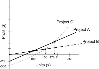
Break-even analysis can also be used to select among alternatives (e.g., projects or construction processes). In order to perform break-even analysis between alternatives, there needs to be a parameter (e.g., cost or revenue variables) that is common in both alternatives. When two alternatives are compared, the break-even point represents the point of indifference between the alternatives (i.e., the point at which two alternatives are equally desirable) (Badiru 1996).
The steps to find the point of indifference between alternatives: Find the common variable between the alternatives
Express the total cost of each alternative as a function of the common variable Equate expressions and solve for the point of indifference
For the example provided in Figure 4, profit functions are graphed. This graph shows that Project B is favorable over the other alternatives if the production is between 0 and 100 units, Project A is favorable if the production is between 100 and 178 units, and Project C is favorable if the production is larger than 178 units.
Figure 4. Plot of profit functions (copyright © Badiru 1996)
Example: There exist two alternative locations for an asphalt mixing plant to transport materials from. Characteristics of these two locations and associated costs are tabulated below. Which location is best for the asphalt mixing plant, the cheaper Location A or closer Location B? (This example has been adopted from MIT Engineering Economics lecture notes, copyright © MIT, Civil and Env. Engineering Department).
Location A Location B
Transportation distance 6 km 4.3 km
Transportation expense $ 1.15/ m3-km $ 1.15/m3-km
Monthly rental expense $ 1000/month $ 5000/month
Set-up cost $ 15 000 $ 25 000
Workmanship costs 0 $ 96/day
Total volume available 50000 m3 50000 m3
Solution:
First obtain the total cost functions for all alternatives
Location A Location B
Fixed Costs
Rental expense 4 month x $1000/month = $ 4000
4 month x $5000/month = $ 20 000
Set-up cost $ 15 000 $ 25 000
Workmanship costs 0 85 days x $96/day = $ 8160
Variable costs
Transportation 6 km x $1.15 x Q 4.3 km x $1.15 x Q
Total Cost $ 19 000 + 6.9 Q $ 53 160 + 4.945 Q
Equate the total cost functions to solve for volume to be transported for break-even point
$ 19 000 + 6.9 Q = $ 53 160 + 4.945 Q Q = 17473 m3.
SUPPLEMENTARY EXAMPLES
Example 1:
A contractor finds that he can buy from a concrete manufacturer, components for 800 TL per unit. Alternatively, he can manufacture the same size and quality components for a variable cost of 400 TL/unit. It is estimated that the additional fixed cost in the plant would be 1 200 000 TL per year, if the components are manufactured by himself. What is the break-even point?
Solution 1:
Total annual cost as a function of the number of units for the make alternative: TCMake = 1 200 000 TL + 400 Q (Q refers to the number of units)
Total cost for the buy alternative: TCBuy = 800 Q
Break-even volume occurs when TCBuy = TCMake
i.e.,
800 Q = 1 200 000 TL + 400 Q, solving for Q will give Q= 3000 units/year.
Example 2:
A special equipment is needed for a specific construction activity at a job site. This equipment can be leased for 5000 TL/day including its cost of maintenance. Alternatively, the equipment can be purchased for 2 500 000 TL. The equipment is estimated to have a useful life of 12 years with a salvage value of 400 000 TL at the end of its useful time. It is estimated that annual maintenance costs will be 300 000 TL. If the interest rate is 6% and it costs 5000 TL per day to operate the equipment, how many days per year are required for the two alternatives to break-even?
Solution 2:
Annual costs of the equipment if leased:
TCL = 5000 Q + 5000 Q (lease + operation costs)
= 10000 Q (Q refers to the number of days per year)
Annual costs of the equipment if purchased:
Break-even occurs when TCL= TCP 10000 Q = 574 530 + 5000 Q Q = 115 days/year
For all the levels of use exceeding 115 days/year it would be more economical to purchase the equipment. If the level of use is anticipated to be below 115 days/year, the computer should be leased, as shown in the following graph.
Example 3:
A hydraulically operated equipment can be fabricated for 140 000 TL and it will have a salvage value of 20 000 TL at the end of 4 years. Maintenance cost will be 12 000 TL/year and the cost of operation will be 85 TL/hr. As an alternative, a mechanically operated equipment can be fabricated for 55 000 TL. This equipment will have no salvage value at the end of a 4 year service life. The cost of operation and maintenance is estimated to be 140 TL/hr.
Solution 3:
Annual equivalent total cost for the hydraulic equipment:
TCH = initial cost – salvage value + maintenance cost + operating costs TCH = 140 000(A/P,10,4) – 20 000 (A/F,10,4) +12 000 +85 Q
(Q refers to the hours of use per year)
TCH = 140 000 x 0.3155 – 20 000 x 0.2155 +12 000 +85 Q TCH = 51 860 + 85 Q
Annual equivalent total cost for the mechanical equipment: TCM = initial cost + operating and maintenance costs TCM = 55 000(A/P,10,4) + 140 Q
TCM = 17 353 + 140 Q
Hydraulic Mechanical
Break –even occurs when TCH = TCM , or
51 860 + 85 Q = 17 353 +140 Q Q = 627 hrs/year
Example 4:
A company manufacturing prefabricated reinforced concrete building elements is operating with an annual cost of 40 000 000 TL, a revenue(income) of 1100 TL/element, and a variable cost of 600 TL/element. The company hopes to produce 100 000 elements per year. What is the break-even point? Would the company make a profit or loss? Assuming that the market is ready for an increase in selling price to 1600 TL/element, how would this affect the yearly profit?
Solution 4:
Break-even point occurs when; Revenue = Cost
1100 Q = 40 000 000 + 600 Q, where Q is the total elements sold in a year. Q = 80000 elements/year
If 100000 elements per year are made and sold, then annual profit will be; Profit = Revenue – cost
Profit = 1100 x 100 000 – 600 x 100 000 – 40 000 000 P = 10 000 000 TL/yr
P = (1600 – 600) x 100 000 – 40 000 000 P = 60 000 000 TL/yr
In other words, if the selling price is increased about 40 to 50%, the annual profit increases by 600%.
Example 5:
The company in Example 4 is considering usage of a new production equipment which will save 3 000 000 TL/year in supervision and related fixed costs. With a revenue of 1100 TL/element, and a variable cost of 600 TL/element, at what volume of production the company starts making profit? What is the expected profit per year for 100 000 units of expected production?
Solution 5: Revenue = Cost
1100 Q = 40 000 000 – 3,000,000 + 600 Q (Q refers to the number of elements per year)
500 Q = 37 000 000 Q = 74000 elements/yr
At 100000 elements per year, the profit will be; P = (1100- 600) x 100 000 – (40 000 000 – 3 000 000)
P = 13 000 000 TL/yr which is greater than 10 000 000 TL/yr when the fixed cost was 40 000 000 TL/yr.
Example 6:
Solution 6:
Break even volume will be at:
40 000 000 + 600 Q = 1125 Q (Q refers to the number of elements per year)
Q = 76 190 elements/yr
At 100000 elements per year, profits will be: P = (1125-600) x 100 000 – 40 000 000
P = 12 500 000 TL/yr >10 000 000 TL/yr when the selling price was 1100 TL/element. The company can spend for the advertisement:
12 500 000 – 10 000 000 = 2 500 000 TL/yr.
References:
Blank, L. T., and Tarquin, A.J. (2008). Engineering Economy”, 5th Edition, McGraw-Hill, USA.
Paek, J. H. (2000). “Running a profitable construction company: Revisited break-even analysis.”
Journal of Management in Engineering, 16(3), 40-46.
Badiru, A. B. (1996). Project Management in Manufacturing and High Technology Operations, Wiley- IEEE, USA.