Particle Gibbs with Ancestor Sampling Methods for Unobserved Component Time Series Models with Heavy Tails, Serial Dependence and Structural Breaks

Munich Personal RePEc Archive

Particle Gibbs with Ancestor Sampling

Methods for Unobserved Component

Time Series Models with Heavy Tails,

Serial Dependence and Structural Breaks

Nonejad, Nima

1 May 2014

Online at

https://mpra.ub.uni-muenchen.de/55664/

Particle Gibbs with Ancestor Sampling Methods for

Unobserved Component Time Series Models with

Heavy Tails, Serial Dependence and Structural Breaks

Nima Nonejad

Aarhus University and CREATES

Abstract

Particle Gibbs with ancestor sampling (PG-AS) is a new tool in the family of sequential Monte

Carlo methods. We apply PG-AS to the challenging class of unobserved component time series

models and demonstrate its flexibility under different circumstances. We also combine discrete

structural breaks within the unobserved component model framework. We do this by modeling

and forecasting time series characteristics of postwar US inflation using a long memory

au-toregressive fractionally integrated moving average model with stochastic volatility where we

allow for structural breaks in the level, long and short memory parameters contemporaneously

with breaks in the level, persistence and the conditional volatility of the volatility of inflation.

Keywords:Ancestor sampling, Bayes, Particle filtering, Structural breaks

(JEL:C11, C22, C52, C63)

∗_{The author acknowledges support from CREATES-Center for Research in Econometric Analysis of Time Series}

1

Introduction

Unobserved component (UC) models are widely used to model time series and dynamical

sys-tems. In this paper we define UC models as a general class of linear, nonlinear, Gaussian and

non-Gaussian state space models that include at least a component that is unobservable. The UC

itself can either be a single continuous component as in section 3 or we can both have a continuous

along with a discrete unobserved component, see section 4. Therefore, our models should not be

confused solely with the UC model of Stock and Watson (2007).

We apply a relatively new tool in the family of sequential Monte Carlo methods which is

partic-ularly useful for inference in UC models, namely, particle Gibbs with ancestor sampling (PG-AS), suggested in Lindsten et al. (2012). PG-AS builds on the particle Gibbs (PG) sampler proposed

by Andrieu et al. (2010). In PG, we start by running a sequential Monte Carlo (SMC) sampler

in which one particle trajectory is set deterministically to a reference trajectory that is specified a

priori. After a complete run of the SMC algorithm, a new trajectory is obtained by selecting one

of the particle trajectories with probabilities given by their importance weights. The effect of the

reference trajectory is that the target distribution of the resulting Markov kernel remains invariant,

regardless of the number of particles used in the underlying SMC algorithm. However, PG

suf-fers from a serious drawback, which is that the underlying mixing can be very poor when there is

path degeneracy in the SMC sampler. In some cases this problem can be addressed by adding a backward simulation step to the PG sampler, yielding a method denoted as PG withbackward simu-lation, see for instance Lindsten and Schön (2013). PG-AS alleviates the path degeneracy problem in a very computationally elegant fashion. Specifically, the original PG kernel is modified using a

so-calledancestor samplingstep. This way the same effect as backward sampling is achieved, but without an explicit backward pass.

In this paper we aim to show that PG-AS provides a very compelling and computationally

fast framework for estimating rather advanced econometric models. We start by reproducing the

results of Chan and Hsiao (2013) which is a book chapter in Bayesian Inference in the Social

Sciences published by John Wiley & Sons. The aforementioned article uses “pure” Gibbs sampling

methods to estimate different stochastic volatility model specifications. We briefly summarize their applications, estimate the same models using PG-AS and compare our results with the results of

Chan and Hsiao (2013). The main difference between Gibbs sampling and PG-AS is that where in

traditional Gibbs sampling problems we resort to converting nonlinear or non-Gaussian models to

linear and Gaussian state space models in order to draw the latent states, in the PG-AS framework

we draw these latent states directly using the nonlinear or non-Gaussian framework.

We also provide extensions where we combine discrete structural breaks within the UC

through irreversible Markov switching or so-called change-point dynamics, see Chib (1998). For

instance, we model time series characteristics of postwar US inflation using a long memory

autore-gressive fractionally integrated moving average model with stochastic volatility where we allow for

structural breaks in the level, autoregressive (AR), moving average (MA) parameters, long memory parameter,d contemporaneously with breaks in the level, persistence and the conditional volatility of the volatility of inflation.

Overall, we believe that applying PG-AS to unobserved component models, especially

struc-tural break specifications is the most important contribution that we make as to our knowledge

there has not yet been any attempts made to use PG-AS in the econometric analysis of these types

of models. As we shall see for these type of models, PG-AS requires limited design effort on the

user’s part especially if one desires to change some features in a particular model. On the other

hand, estimating the same type of models using “pure” Gibbs sampling would require relatively

more programming effort.

The remaining of this paper is as follows: in section 2 we briefly describe the steps of PG-AS.

In sections 3 and 4 we present our empirical applications. Finally, the last section concludes.

2

Particle Gibbs with Ancestor Sampling

Consider the following stochastic volatility (SV) model

yt = µ+exp(ht/2)εt, εt ∼N(0,1) (2.1)

ht = µh+φh(ht−1−µh) +ζt, ζt∼N 0,σh2

(2.2)

whereyt is the observed data,h1:T = (h1, ...,hT)

′

are the unobserved log-volatilities,µ_his the drift term in the state equation, σh is the volatility of log-volatility andφh is the persistence parameter.

Typically, we would impose that |φh| <1 so that we have a stationary process with the initial

condition, h1 ∼N µh,σ_h2/ 1−φ_h2

. We collect the model parameters in θ = µ,µh,φh,σ_h2

′

and letYT = (y1, ...,yT)

′

. The above stochastic volatility model is an example of a nonlinear state

space model where the measurement equation, (2.1) is nonlinear in the states, h1:T. The major

challenge of estimating this model is that while sampling p(θ |h1:T,YT)is relatively easy, sampling

h1:T ∼p(h1:T |θ,YT)is often difficult.

Within the Gibbs sampling framework, the most popular approach for estimating (2.1)-(2.2) is

the so-called auxiliary mixture sampler, see Kim et al. (1998). The idea is to approximate the

non-linear stochastic volatility model using a mixture of non-linear Gaussian models. Specifically, we can

square both sides of (2.1) and take the logarithm such that y∗_t =ht+εt∗ where yt∗=log(yt−µ)2

and ε_t∗ = logε2

t. Kim et al. (1998) show that εt∗ can be approximated by a seven-component

variable, zt ∈ {1, ...,7} that serves as a mixture component indicator. Hence, εt∗|zt ∼N mi,s2i

with p(zt=i) =ωi. The values of mi, s2i and ωi, i=1, ...,7 are all fixed and given in Kim et

al. (1998). Using this Gaussian mixture approximation the SV model can be expressed as a linear

Gaussian state space model. Bayesian estimation can then be performed using standard Gibbs sam-pling techniques for linear Gaussian state space models, see for instance Kim and Nelson (1999).

Finally, notice that using this specification we sample from the posterior, p(θ,h1:T,z1, ...,zT |YT)

augmented to includez1, ...,zT and not fromp(θ,h1:T |YT).

Within the PG-AS framework we need not use the above approximation. On the contrary, we

approach estimating (2.1)-(2.2) directly by first drawingh1:T ∼p(h1:T |θ,YT)using the conditional

particle filter with ancestor sampling. Thereafter, we draw p(θ |h1:T,YT). Notice that once we

obtainh1:T, sampling each element ofθ is straightforward. In the following we describe the steps

of the conditional particle filter with ancestor sampling (CPF-AS) which is used to drawh1:T from

p(h1:T |θ,YT). For more details the reader is referred to Lindsten et al. (2012). Let i=1, ...,N

denote the number of Gibbs sampling iterations, j=1, ...,M denote the number of particles and let p(yt |θ,ht,Yt−1) denote the density of yt given θ, ht andYt−1. Finally, let h(_1:i−_T1) be a fixed

reference trajectory ofh1:T sampled at iterationi−1 of the Gibbs sampler. The steps of CPF-AS

(particle filter conditional onh(_1:i−_T1)) for the SV model are as follows

1. ift=1

(a) Drawh(₁j)|h₀(j),θ for j=1, ...,M−1 and sethM₁ =h(₁i−1). (b) Setw(₁j)=τ₁(j)/Σ_kM₌₁τ₁(k) whereτ₁(j)=p

y1|θ,h

(j)

1 ,Y0

for j=1, ...,M.

2. else fort=2toT do

(a) Resamplenh_t(₋j)₁

oM−1

j=1 using indicesa

(j)

t where p

a_t(j)= j

∝w(_t−j)₁for j=1, ...,M−1.

(b) Drawh_t(j)|h

at(j)

t−1 ,θ for j=1, ...,M−1.

(c) SethM_t =h(_ti−1).

(d) Drawa_t(M)frompa_t(M)= j∝w(_t−j)₁ph(_ti−1)|h_t(₋j−₁1),θ.

(e) Seth(_1:j_t)= h

a(tj)

1:t−1,h

(j)

t

!

,w_t(j)=τ_t(j)/Σ_kM₌₁τ_t(k)whereτ_t(j)= p

yt|θ,h

(j)

t ,Yt−1

.

3. end for

4. Sampleh(_1:i)_T |θ,YT withp

h_1:(i)_T =h_1:(j_T) |θ,YT

∝w(_Tj).

Even though this is a small modification of the algorithm, improvements in mixing can be quite

considerable, see Lindsten et al. (2012). Once we sample h1:T, we use standard methods and

sample each element ofθ, see for instance Kim et al. (1998) and Chan and Hsiao (2013).

Extending the standard SV model within the PG-AS framework is straightforward. For exam-ple, assume that εt ∼St(v), whereSt stands for the Student-t distribution with v>2 degrees of

freedom. For this specification, at the ith iteration of the Gibbs sampler for p(yt |θ,ht,Yt−1) we

can use

p(yt |θ,ht,Yt−1) =

Γ v+₂1 Γ v₂ p

(v−2)π

1

σt

1+ (yt−µ)

2

(v−2)σ2

t

!−(v+1)/2

(2.3)

inside the CPF-AS algorithm and obtain h(_1:i)_T. We then sample µ(i)_{, µ}(i)

h , φ

(i)

h andσ

2(i)

h as in Chan

and Hsiao (2013). Finally, in order to draw v(i) ∼ pv|µ(i)_,h(i)

1:T,YT

we use (2.3) and

per-form Metropolis-Hastings (M-H). Hence, we generate a candidatev∗fromq(v)∼T N_]2,∞[(vˆML,V)

where T N_]2,∞[ stands for the truncated Normal density on the domain ]2,∞[ and ˆvML is obtained

by maximizing (2.3) with respect to vusing the already obtained values of h(_1:i)_T and µ(i)_{. We set}

V =c·var(vˆML), wherec∈R+ and fine-tuneV by adjustingcsuch that we can get a decent M-H

acceptance ratio around 50 to 60%. We then drawufrom a standard Uniform distribution,U and acceptv∗, i.e.v(i)=v∗ifaMH

v∗,v(i−1)>uwhere

aMH

v∗,v(i−1)

= min    1,

pv∗|µ(i)_,h(i)

1:T,YT

qv(i−1) pv(i−1)_|µ(i)_,h(i)

1:T,YT

q(v∗)

 



(2.4)

else we set v(i) =v(i−1). On the other hand, if we were to use pure Gibbs sampling to estimate the SV model with Student-t distributed errors then we would be forced to follow Chan and Hsiao

(2013) and convert the model into a conditionally Gaussian state space model by defining the

measurement error in (2.1) asεt =λ−

1/2

t et whereet∼N(0,1),λt∼IG(v/2,v/2)and has a closed

form conditional posterior. We would then follow the steps in Chan and Hsiao (2013) and sample

from the augmented posterior, p(θ,v,h1:T,λ1, ...,λT,z1, ...,zT |YT).

2.1

Model comparison using the output from PG-AS

One of the main outputs from CPF-AS is the loglikelihood ofYT withh1:T integrated out,p(YT |θ).

This quantity is the product of the individualintegratedlikelihood contributions

p(YT |θ) = T

∏

t=1

(2.5) can be used to for instance compute the marginal likelihood (ML) for a particular model. The

marginal likelihood is defined as

p(YT) =

ˆ

Θ

p(YT |θ)p(θ)dθ (2.6)

and is a measure of the success the model has in accounting for the data after the parameter

uncer-tainty has been integrated out over the prior, p(θ).

Gelfand and Dey (1994) propose a very compelling and general method to calculate ML. It is

efficient and utilizes the same routines when calculating ML for different models. The Gelfand-Dey

(G-D) estimate of the marginal likelihood is based on

1

N

N

∑

i=1

gθ(i)/hpYT |θ(i)

pθ(i)i → p(YT)−1 as N →∞ (2.7)

where N is the number of PG-AS iterations. Gelfand and Dey (1994) show that if gθ(i) is thin-tailed relative to p

YT |θ(i)

p

θ(i)_{then (2.7) is bounded and the estimator is consistent.} Following Geweke (2005) a truncated Normal distribution,N(θ∗,Σ∗)is used forg(θ). The quan-tities θ∗ and Σ∗ are the posterior sample moments calculated as θ∗ =N−1ΣN

i=1θ(i) and Σ∗ =

N−1ΣN i=1

θ(i)_−θ∗ _θ(i)_−θ∗ ′

whenever θ(i) _{is in the domain of the truncated Normal. This} domain,Θis defined as

Θ =

θ : θ(i)−θ∗

′

(Σ∗)−1θ(i)−θ∗≤χ_α2(z)

wherezis the dimension of the parameter vector andχ2

α(z)is theαth percentile of the Chi-squared

distribution with z degrees of freedom. In practice, 0.5, 0.75, 0.95 and 0.99 are popular selec-tions for α. Once the marginal likelihood for different specifications has been calculated, we

can compare them using Bayes factors, BF. The relative evidence for model M_{A versus} M_{B is}

BFM_AB =p(YT |MA)/p(YT |MB). This odds ratio is the factor by which the data considersMA

more probable than M_{B. Kass and Raftery (1995) recommend considering twice the logarithm of}

the Bayes factor for model comparison and suggest a rule-of-thumb of support forM_{A based on}

2 logBFM_AB: 0 to 2 not worth more than a bare mention, 2 to 6 positive, 6 to 10 strong, and greater

than 10 as very strong.

We can also use p(YT |θ) and compute the deviance information criterion (DIC) of

Spiegel-halter et al. (2002). DIC is a compelling alternative to AIC or BIC and it can be applied to

nested or non-nested models. Calculation of DIC in a PG-AS scheme is trivial. Contrary to

of p(YT |θ)and a penalty term, pDwhich describes the complexity of the model and serves as a

penalization term that corrects deviance’s propensity toward models with more parameters. More

precisely, pD=D(θ)−D θ¯

where D(θ)is approximated by N−1ΣN_i=1−2 logp

YT |θ(i)

and

D θ¯

=−2 logp YT |θ¯. ¯θ is estimated from the PG-AS output using the mean or mode of the

posterior draws. The DIC is defined asD θ¯

+2pD.

It is worth noting that the best model is the one with the smaller DIC. Very roughly, for

differ-ences of more than 10 we might definitely rule out the model with the higher DIC.

3

Stochastic Volatility Models

In this section we start by estimating the basic stochastic volatility model, (2.1)-(2.2) using PG-AS.

Thereafter, we extend the SV model to allow for moving average errors and heavy tails.

Further-more, for each specification we compare our results to the results of Chan and Hsiao (2013)1. We use the exact data and prior settings as Chan and Hsiao (2013). Thus, we ought to be

able to compare the performance of PG-AS with traditional Gibbs sampling in a rather easy and

intuitive way. As stated earlier, the main difference between the Gibbs sampling approach of Chan

and Hsiao (2013) and PG-AS is that where Chan and Hsiao (2013) resort to converting nonlinear

or non-Gaussian models to linear and Gaussian state space models in order to draw h1:T, in the

PG-AS framework we drawh1:T directly from p(h1:T |θ,YT)using the nonlinear or non-Gaussian

framework. In the following we briefly summarize their applications labeled as (1), (2) ,(3) and

reproduce their results using PG-AS:

(1) Modeling daily AUD/USD exchange rate returns from January 2005 to December 2012

using (2.1)-(2.2).

(2)Modeling daily PHP/USD exchange rate returns from July 2007 to December 2012 using a

moving average stochastic volatility (MASV) model. This model is defined as

yt = µ+eht/2εt+ψ1eht−1/2εt−1, εt∼N(0,1)

ht = µh+φh(ht−1−µh) +ζt, ηt ∼N 0,σh2

where εt is independent from ζt. Furthermore, for identification, we impose that the root of the

characteristic polynomial associated with the MA coefficient, ψ1 is outside the unit circle.

Com-pared to (2.1)-(2.2) we have an additional parameter,ψ1. The conditional posterior ofψ1does not

have a closed form solution. Therefore, we sampleψ1using Metropolis-Hastings. We follow Chan

and Hsiao (2013), choose the prior forψ1as a standard Normal truncated in the interval]−1,1[and

employ rejection sampling to ensure thatψ₁(i)∈]−1,1[.

(3)Modeling daily returns on the silver spot price from January 2005 to December 2012 using

a moving average stochastic volatility model with Student-t distributed errors, MASVt

yt = µ+eht/2εt+ψ1eht−1/2εt−1, εt∼St(v)

ht = µh+φh(ht−1−µh) +ζt, ηt∼N 0,σh2

For each of these models we use the exact same prior hyperparameter values as Chan and Hsiao

(2013) to sample θ and ψ1 from their respective conditional posteriors. With regards to v, we

choosep(v)∼U(2,128), whereUstands for the Uniform distribution with lower (upper) endpoint of 2(128) and samplevusing (2.4), see also Chib et al. (2002). Finally, since p(YT |θ) is easily

available from the particle filter, we also report the logarithm of the marginal likelihood, log(ML)

and DIC. We setM=100 and follow Chan and Hsiao (2013) obtainingN=20000 draws from the posterior distribution, after a burn-in period of 1000. The PG-AS estimates along with the original

results of Chan and Hsiao (2013) are reported in Tables 1 to 3. Overwhelmingly, these estimates

are very similar to the Gibbs sampling estimates of Chan and Hsiao (2013), referred to and labeled as “MCMC” in the text below.

In the top row of Figure 1 we compare posterior estimates of exp(ht/2), t =1, ...,T for the

SV model using AUD/USD returns. The left-hand-side displays the posterior mean (solid line)

and 90% credibility intervals (dashed lines) for PG-AS while the right-hand-side displays the same

quantities for the Gibbs sampling algorithm of Chan and Hsiao (2013). We see that these estimates

are basically identical. To further compare the performance of the samplers, we also report the

inefficiency factors, RB of the posterior draws of θ, ψ1, v, h1:T for PG-AS and Chan and Hsiao

(2013). RB is defined as

RB = 1+

2B B−1

B

∑

l=1

K

l B

ˆ

ρ(l)

where ˆρ(l) is an estimate of the autocorrelation at lag l of the sampler, B is the bandwidth and

K is the Parzen Kernel, see also Kim et al. (1998) for a further background on this measure. RB

displays the relative variance of the posterior sample draws when adapting for correlation between

iterations, as compared to the variance without accounting for correlation and serves as a useful

diagnostic for measuring how well the chain mixes. In these calculations, we choose a bandwidth,

Bof 100. Overall, we see that both methods perform similarly forθ,ψ1andvasRBdoes not vary

that much across estimation methods. However, note that forh1:T each vector is of lengthT, so we

have a total of 2T inefficiency factors for each application. Therefore, we use box plots to report this information. In panels (c) and (d) of Figure 1 we report results for AUD/USD with similar

Table 1: Posterior mean (mean), standard deviation (std. dev), 5%-tile and 95%-tile of the model parameters, AUD/USD daily returns data

Parameter mean std. dev 5%-tile 95%-tile RB

Original results, Chan and Hsiao (2013)

µ -0.029 0.013 -0.051 -0.006 1.496

µ_h -0.748 0.351 -1.275 -0.229 1.094

φh 0.989 0.004 0.982 0.995 12.248

σ2

h 0.017 0.003 0.012 0.023 43.519

Reproducing original results using PG-AS

µ -0.029 0.013 -0.052 -0.007 1.567

µh -0.713 0.354 -1.239 -0.197 1.154

φ_h 0.989 0.004 0.982 0.996 13.147

σ2

h 0.018 0.003 0.012 0.024 47.231

log(ML)

α=0.99

-2336.395

DIC 4640.389

RB: inefficiency factors (using a bandwidthBof 100). log(ML): logarithm of the marginal likelihood for the corre-sponding value ofα. DIC: deviance information criterion.

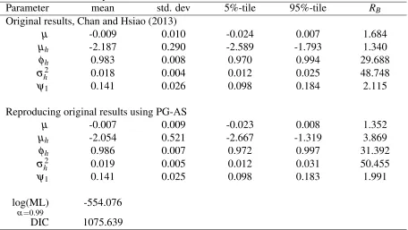
Table 2: Posterior mean (mean), standard deviation (std. dev), 5%-tile and 95%-tile of the model parameters, PHP/USD daily returns data

Parameter mean std. dev 5%-tile 95%-tile RB

Original results, Chan and Hsiao (2013)

µ -0.009 0.010 -0.024 0.007 1.684

µ_h -2.187 0.290 -2.589 -1.793 1.340

φh 0.983 0.008 0.970 0.994 29.688

σ2

h 0.018 0.004 0.012 0.025 48.748

ψ1 0.141 0.026 0.098 0.184 2.115

Reproducing original results using PG-AS

µ -0.007 0.009 -0.023 0.008 1.352

µ_h -2.054 0.521 -2.667 -1.319 3.869

φh 0.986 0.007 0.972 0.997 31.392

σ2

h 0.019 0.005 0.012 0.031 50.455

ψ1 0.141 0.025 0.098 0.183 1.991

log(ML)

α=0.99

-554.076

DIC 1075.639

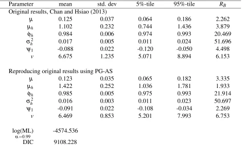
Table 3: Posterior mean (mean), standard deviation (std. dev), 5%-tile and 95%-tile of the model parameters, silver spot price daily returns data

Parameter mean std. dev 5%-tile 95%-tile RB

Original results, Chan and Hsiao (2013)

µ 0.125 0.037 0.064 0.186 2.262

µ_h 1.102 0.232 0.744 1.436 3.879

φh 0.984 0.006 0.974 0.993 20.469

σ2

h 0.017 0.005 0.011 0.024 51.696

ψ1 -0.088 0.022 -0.120 -0.050 4.498

v 6.675 1.235 5.071 8.894 6.153

Reproducing original results using PG-AS

µ 0.123 0.035 0.065 0.182 3.335

µh 1.422 0.252 1.036 1.781 1.933

φh 0.985 0.005 0.975 0.993 21.914

σ_h2 0.016 0.003 0.011 0.023 50.697

ψ1 -0.091 0.022 -0.108 -0.034 2.269

v 6.469 0.853 5.201 7.993 6.753

log(ML)

α=0.99

-4574.536

DIC 9108.228

RB: inefficiency factors (using a bandwidthBof 100). log(ML): logarithm of the marginal likelihood for the corre-sponding value ofα. DIC: deviance information criterion.

and upper lines represent respectively the 25% and 75%-tiles. The whiskers extend to the maximum and minimum. For example, the box plot associated withh1:T for PG-AS (MCMC) indicates that

about 75% of the log-volatilities have inefficiency factors less than 1.6 (3.75), and the maximum

is close to 2.1 (4.8). Overall, results suggest that PG-AS is quite efficient in terms of producing

posterior draws ofh1:T that are not highly autocorrelated. Furthermore, we see that PG-AS provides

better mixing compared to MCMC forh1:T asRB is on average lower.

[Figure1 about here]

Overall, with regards to reproducing the results of Chan and Hsiao (2013) we find that the only

minor difference between PG-AS and Gibbs sampling estimates is in µh for the MASVt model

as PG-AS estimates µh at a higher rate. However, this does not affect any qualitative conclusions

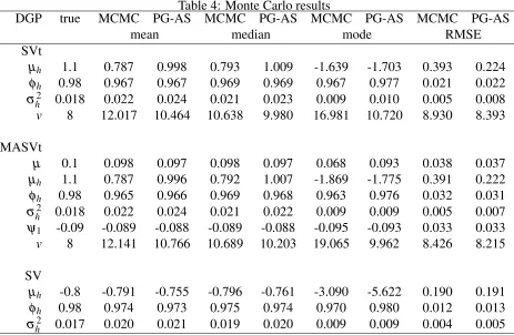
drawn from the results. In order to explore this difference we perform a Monte Carlo analysis.

We consider two data generating processes (DGP), one for a SVt model and one for a MASVt

model. We generate 100 data sets of T =1000 observations for each case, re-estimate, compare the estimated parameters of PG-AS and MCMC with the parameters under the DGP. We choose the

estimation we use the codes of the authors. For each DGP we first generateh1:T through (2.2) with

h1 ∼N µh,σ_h2/ 1−φ_h2

. Thereafter, we use εt ∼St(v) and generate yt. Given a full PG-AS

and MCMC run we calculate the mean, median and mode of the posterior draws, θ(i), i=1, ...N. We then take the mean of these quantities over the number of Monte Carlo repetitions. We also consider the root mean squared error (RMSE), defined as

RMSE =

v u u t

1 100

1

N

100

∑

r=1

N

∑

i=1

θr(i)−θ

2

where θr(i) is the ith posterior draw of the rth Monte Carlo repetition and θ is the vector of the

true DGP parameters. Results are summarized in Table 4. Overall, both methods work very well. However, in both cases we notice reductions in the RMSE ofµ_hby about 75% when we use PG-AS compared to MCMC. More importantly, as for the silver data, in the Monte Carlo repetitions we

(correctly) estimate µ_h at a higher rate using PG-AS compared to MCMC. Furthermore, we also see a slight reduction in the RMSE ofvfor PG-AS compared to MCMC. Thus, Monte Carlo results show that we can be very confident with regards to using PG-AS. We also repeat this Monte Carlo

for a plain SV model and report the results in the bottom part of Table 4. Here, we do not find any

differences worth mentioning.

Table 4: Monte Carlo results

DGP true MCMC PG-AS MCMC PG-AS MCMC PG-AS MCMC PG-AS

mean median mode RMSE

SVt

µh 1.1 0.787 0.998 0.793 1.009 -1.639 -1.703 0.393 0.224

φ_h 0.98 0.967 0.967 0.969 0.969 0.967 0.977 0.021 0.022

σ2

h 0.018 0.022 0.024 0.021 0.023 0.009 0.010 0.005 0.008

v 8 12.017 10.464 10.638 9.980 16.981 10.720 8.930 8.393

MASVt

µ 0.1 0.098 0.097 0.098 0.097 0.068 0.093 0.038 0.037

µh 1.1 0.787 0.996 0.792 1.007 -1.869 -1.775 0.391 0.222

φ_h 0.98 0.965 0.966 0.969 0.968 0.963 0.976 0.032 0.031

σ2

h 0.018 0.022 0.024 0.021 0.022 0.009 0.009 0.005 0.007

ψ1 -0.09 -0.089 -0.088 -0.089 -0.088 -0.095 -0.093 0.033 0.033

v 8 12.141 10.766 10.689 10.203 19.065 9.962 8.426 8.215

SV

µh -0.8 -0.791 -0.755 -0.796 -0.761 -3.090 -5.622 0.190 0.191

φ_h 0.98 0.974 0.973 0.975 0.974 0.970 0.980 0.012 0.013

σ2

h 0.017 0.020 0.021 0.019 0.020 0.009 0.009 0.004 0.005

Finally, in Figure 2 we plot the marginal posterior densities using the output of PG-AS for the

MASVt model using the silver data. The marginal posteriors are bell shaped and centered around

the mean. We also report Markov chain output of the model parameters. The chain mixes well with

relatively fast decaying autocorrelation functions.

[Figure2 about here]

3.1

Sensitivity of PG-AS with respect to

M

We often find that the choice ofM is important because it ensures that the estimate of h1:T is not

too jittery or imprecise. Therefore, we experiment with different values of Mto find out its effect on estimation results. We do this by considering a more challenging specification than (2.1)-(2.2).

From a computational point of view, this extension also allows us to demonstrate the flexibility of

PG-AS to adapt to more complicated model structures without any major computational costs.

Specifically, we consider the stochastic volatility in mean (SVM) model of Koopman and Hol

Uspensky (2002). Hence, in this specification, eht _{appears in both the conditional mean and the}

conditional variance. We follow the same notation as before and define the SVM model as

yt = µ+λexp(ht) +exp(ht/2)εt, εt ∼N(0,1) (3.1)

where ht follows (2.2). Estimation of this specification is nontrivial using pure Gibbs sampling.

This is because drawingh1:T ∼ p(h1:T |θ,λ,YT)is computationally more demanding as (3.1) and

(2.2) cannot be written in linear state space form, see for instance Chan (2014). However, within the

PG-AS context, estimating the SVM model is straightforward. We note that p(yt|θ,λ,ht,Yt−1)∼

N(µ+λexp(ht),exp(ht)). Incorporating this specification is very easy in CPF-AS as we only

need to modify step (e) of the algorithm and use τ_t(j)=N

µ+λexph_t(j)

,exph(_tj)

instead

of τ_t(j) =Nµ,exph_t(j) in the case of the SV model. The PG-AS sampler then provides us withh1:T conditional onθ, λ andYT. Furthermore, we add another layer to our sampler and also

sampleλ |µ,h1:T,YT from its conditional posterior.

We simulate yt, t =1, ...,1000 using (3.1)-(2.2). Thereafter, we re-estimate the SVM model

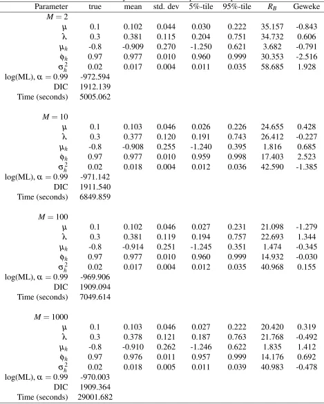
using our simulated data forM=2,10,100 and 1000. We report parameter estimates of the SVM model using the above mentioned number of particles in Table 5. Besides these estimates we

also report the inefficiency factors (RB) of the parameters andh1:T for each case, see Figure 3.

Furthermore, we compute Geweke’s convergence statistics and present estimation time (in seconds)

of the SVM model for eachM. In each case, we sample N=20000 draws from p(θ,λ,h1:T |YT)

Table 5: Sensitivity of the PG-AS sampler with respect toM

Parameter true mean std. dev 5%-tile 95%-tile RB Geweke

M=2

µ 0.1 0.102 0.044 0.030 0.222 35.157 -0.843

λ 0.3 0.381 0.115 0.204 0.751 34.732 0.606

µ_h -0.8 -0.909 0.270 -1.250 0.621 3.682 -0.791

φh 0.97 0.977 0.010 0.960 0.999 30.353 -2.516

σ2

h 0.02 0.017 0.004 0.011 0.035 58.685 1.928

log(ML),α =0.99 -972.594 DIC 1912.139 Time (seconds) 5005.062

M=10

µ 0.1 0.103 0.046 0.026 0.226 24.655 0.428

λ 0.3 0.377 0.120 0.191 0.743 26.412 -0.227

µ_h -0.8 -0.908 0.255 -1.240 0.395 1.816 0.685

φh 0.97 0.977 0.010 0.959 0.998 17.403 2.523

σ2

h 0.02 0.018 0.004 0.012 0.036 42.590 -1.385

log(ML),α =0.99 -971.142 DIC 1911.540 Time (seconds) 6849.859

M=100

µ 0.1 0.102 0.046 0.027 0.231 21.098 -1.279

λ 0.3 0.381 0.119 0.194 0.757 22.693 1.344

µ_h -0.8 -0.914 0.251 -1.245 0.351 1.474 -0.345

φh 0.97 0.977 0.010 0.960 0.999 14.932 -0.030

σ2

h 0.02 0.017 0.004 0.012 0.035 40.968 0.155

log(ML),α =0.99 -969.906 DIC 1909.094 Time (seconds) 7049.614

M=1000

µ 0.1 0.103 0.046 0.027 0.222 20.420 0.319

λ 0.3 0.378 0.121 0.187 0.763 21.768 -0.492

µ_h -0.8 -0.910 0.262 -1.246 0.622 1.835 1.412

φh 0.97 0.976 0.011 0.957 0.999 14.176 0.692

σ2

h 0.02 0.018 0.005 0.011 0.039 40.983 -0.478

log(ML),α =0.99 -970.003 DIC 1909.364 Time (seconds) 29001.682

Overall, we see that PG-AS performs very well as parameter estimates are close to their respective

DGP values. Furthermore, the choice ofM=100 is very sensible. In fact, we get almost identical results for M=10 and M=100 but RB falls as we set M=100. For instance, in Figure 3, for

M=10, 75% ofh1:Ts have inefficiency factors less than 8 while forM=100 this number is close

to 2. Compared to M=100 we do not obtain any significant gains inRB when we setM=1000.

However, asMincreases the computation time also increases and from this point of viewM=1000 seems computationally very demanding.

[Figure3 about here]

4

Structural Breaks and PG-AS

In this section we demonstrate the flexibility of PG-AS by combing PG-AS with the change-point

specification of Chib (1998). Specifically, we believe that this combination is in fact the most

important contribution that we make since relatively only few papers have dealt with combining

models with SV effects with what in the literature is considered as a “state-of-the-art” structural

break model.

We start by using a linear regression Markov switching model with a specific structure on the transition probabilities combined with SV effects. Testing for the number of regimes,m∈ {1,2, ...}

is then a test for the number of structural breaks, see Chib (1998). We follow Liu and Maheu

(2008) and estimate each model conditional on 0,1, ...mbreaks occurring in the sample. For each of these we calculate ML (DIC) and use them to determine the optimal number of change points.

Specifically, we can compare marginal likelihoods using Bayes factors and use differences in the

DIC between different specifications to determine the number of structural breaks.

The m-state MS linear regression model with SV effects which allows for m−1 structural breaks in the regression coefficients and level of volatility is defined as

yt = Xt−1βst+εt, εt∼N

0,γsteht

(4.1)

ht = φhht−1+ζt, ζt ∼N 0,σh2

(4.2)

wherest=1, ...,m,s1:T = (s1, ...,sT)

′

andst=kindicates thatytis from regimek. In section 4.3 we

also consider structural breaks inφhandσ_h2. Incorporating breaks inφhandσ_h2is straightforward

as we can use the conditioning features of PG-AS and thus sample these parameters using the

log-volatilities within each regime. As before, YT = (y1, ...,yT)

′

is T×1, XT is a T×n matrix

of regressors with row Xt−1 which can also include lags of yt and βst is n×1. The parameter

γst =exp µh,st

probability matrix forst is assumed to be P =         

p11 p12 0 · · · 0

0 p22 p23 · · · 0

..

. ... ... ... ... ..

. ... 0 pm−1,m−1 pm−1,m

0 0 · · · 0 1

         (4.3)

where plk= p(st =k|st−1=l)withk=l ork=l+1 is the probability of moving from regimel

at timet−1 to regimekat timet. Pensures that givenst=kat timet, the next periodt+1,st+1

remains in the same state or jumps to the next state. For instance, givenst=k, one has thatst+1=k

orst+1=k+1 with pk,k+pk,k+1=1. Once the last regime is reached, we stay there forever, that

is pm,m=1. This structure enforces the following ordering

θ =                 

θ1 if t<τ1 θ2 if τ1≤t<τ2

..

. ... ...

θm−1 if τm−2≤t<τm−1 θm if τm−1≤t

where θk = (βk,γk)

′

, k=1, ...,m, θ = {βk}mk=1,{γk}mk=1,φh,σ_h2

′

and τ1,τ2, ...,τm−1 are the

un-known structural break dates. Modeling (4.1)-(4.2) using (4.3) is straightforward as we can use the

conditioning features of PG-AS. Specifically, we proceed by cycling through the following steps

1. s1:T |β =β1, ...,βm,γ =γ1, ...,γm,φh,σ_h2,P,YT

2. h1:T |β1, ...,βm,γ1, ...,γm,φh,σh2,s1:T,YT

3. β1, ...,βm|γ1, ...,γm,h1:T,s1:T,YT

4. γ1, ...,γm|β1, ...,βm,h1:T,s1:T,YT

5. φh|σ_h2,h1:T

6. σ2

h |φh,h1:T

7. P|s1:T

In step 1, we use the algorithm of Chib (1998) to draws1:T, see for instance Liu and Maheu (2008).

previous Gibbs iteration. The parameters:β,γ,φhandσ_h2are all sampled using standard techniques

conditional on the newly draws of s1:T andh1:T. The conditional posterior of pkk, k=1, ...,m−1

isBeta(a0+nkk,b0+1)wherenkk is the number of one-step transitions from statekto statekin a

given sequence ofs1:T.

We use N(0n,In) prior for βk, γk ∼IG 4₂,0₂.2

, φ_h ∼Beta(20,1.5), σ2

h ∼IG

4 2,

0.2 2

where

IG ₂.,₂.

stands for the Inverse-gamma density, see Kim and Nelson (1999). Finally, with regards

to pkk, we choose pkk ∼Beta(a0=20,b0=0.1)for k=1, ...,m−1. We start with a simulation

example in section 4.1 and then provide an empirical application using real US GDP growth rate.

4.1

Simulation example

Consider data generated according to the following model

yt = 1+εt, εt∼N

0,1.4eht for 1≤t<100

yt = 0.1+εt, εt∼N

0,0.2eht for t≥100

whereht=0.9ht−1+ζt andζt ∼N(0,0.02)fort =1, ...,200. We estimate the above model

con-ditional onm=0,1,2 change points and determine the optimal number of change points using ML and DIC. Furthermore, notice that in order to obtain p(YT |θ,P)we use that

logp(YT |θ,P) = T

∑

t=1

logp(yt|θ,P,Yt−1)

where

p(yt |θ,P,Yt−1) =

m

∑

k=1

p(yt|θ,Yt−1,st=k)p(st=k|θ,P,Yt−1)

The first term, p(yt |θ,Yt−1,st=k)is obtained from CPF-AS usingθk= (βk,γk)

′

,φ_h, σ2

h and the

last term is computed from

p(st =k|θ,P,Yt−1) =

k

∑

l=k−1

p(st−1=l|θ,P,Yt−1)plk, k=1, ...,m

p(st=k|θ,P,Yt) =

p(st=k|θ,P,Yt−1)p(yt |θ,Yt−1,st =k)

∑m_l=1p(st=l|θ,P,Yt−1)p(yt|θ,Yt−1,st=l)

, k=1, ...,m(4.4)

The last equation is obtained from Bayes’ rule. Note that in (4.4) the summation is only fromk−1 tok, due to the restricted nature of the transition matrix.

log(ML) and DIC for specifications with no change point up to two change points. As expected, the

specification with one change point obtains the highest (lowest) ML (DIC). We also compute the

marginal likelihood for the change-point models using the method of Sims et al. (2008) because

as pointed out in Sims et al. (2008) the G-D method may not work for models with time-varying parameters as the posterior density tends to be non Gaussian. However, we do not find any

signif-icant changes compared to G-D. Therefore, we choose to retain these values. We also conduct a

Monte Carlo analysis (not reported) generating data from (4.1)-(4.2) for 0, ..,mchange points and comparing ML between different specifications. Results indicate that the G-D method correctly

identifies the true number of structural breaks at almost every Monte Carlo iteration.

Table 6: Change-point stochastic volatility model # CP log(ML)

α=0.50

log(ML)

α=0.75

log(ML)

α=0.95

log(ML)

α=0.99

DIC

0 -266.721 -266.430 -266.291 -266.278 509.786 1 -242.227 -242.303 -242.112 -242.074 445.991 2 -252.231 -251.926 -251.716 -251.677 467.307

This table displays the full sample marginal likelihood and DIC estimates for the change-point stochastic volatility model. # CP is the number of change points that are conditioned on.

We compare the performance of our model (break) to a recursive OLS specification (no-break).

The top panel of Figure 4 shows the predictive mean of these models along withyt. Both predictive

means are similar before the break att =100. However, after the break, we see a quick reduction in the predictive mean from the break model while the predictive mean from the no-break model

remains high for a long time. In the top right panel, we plot the density of the change point along

with the true position of the change point. Clearly, our model is able to detect the date of the structural break. We also compare our estimates of σ2

t = γstexp(ht), t = 1, ...,T with the true

conditional variance process. In panel (f), we plot the marginal posterior densities ofγ1andγ2. The

marginal posteriors are bell shaped and centered around their means (1.34 forγ1and 0.15 forγ2).

We also report the Markov chain output and autocorrelation function for γ1|YT and γ2|YT. The

chain mixes well with relatively fast decaying autocorrelation functions.

[Figure4 about here]

Finally, Table 7 displays out-of-sample results for one-period-ahead direct forecasts (see Marcellino et al. (2005)) for the no-break and the break model. In the context of forecasting with the break

model we perform the following: for the first out-of-sample observation at timet we calculate ML for 1 and 2 change points usingYt−1. Thereafter, we choose the optimal change-point number,n1

using Bayes factors and calculate the predictive mean,E[yt|Yt−1]using the parameters associated

ML for 1 and 2 change points, choose the optimal n2and repeat the above forecasting procedure

to obtain E[yt+1|Yt]. Furthermore, in addition to MAE and RMSE, forecasts are also compared

using the linear exponential (LINEX) loss function of Zellner (1986). This loss function is defined

asL(yt,yˆt) =b[exp(a(yˆt−yt))−a(yˆt−yt)−1], where ˆyt is the forecast. L(yt,yˆt)ranks

overpre-diction (underpreoverpre-diction) more heavily fora>0(a<0). The table includesb=1, witha=1 and

a=−1.

Table 7: Out-of-sample forecasts

Model MAE RMSE LINEX,a=1,b=1 LINEX,a=−1,b=1

No-break 0.779 0.916 0.452 0.553

Break 0.528 0.722 0.305 0.340

This table reports mean absolute error (MAE) and root mean squared error (RMSE) for the forecasts based on the predictive mean for one-step-ahead. Furthermore, average LINEX loss function is reported for a=1, a=−1 and

b=1. The out-of-sample period is fromt=51, ...,200.

Overall, the break model offers improvements in terms of MAE and RMSE compared to the no-break model. When the LINEX loss function is used, the no-break model’s ability to capture variations

in higher moments provides gains in terms of point forecasts.

4.2

Real output

Recent literature documents a structural break in the volatility of US GDP growth rate, see for

instance Kim and Nelson (1999) and Gordon and Maheu (2008). In this section we follow Gordon

and Maheu (2008) and consider structural break estimates of AR(2) models in real US GDP growth

rate using the framework of (4.1)-(4.2).

Letyt=100[log(qt/qt−1)−log(pt/pt−1)], whereqt is quarterly US GDP seasonally adjusted

and pt is the US GDP price index. Our data ranges from 1947q4 to 2013q3, for a total of 264

observations. In the following we compare the performance of (4.1)-(4.2) with 2 lags ofyt, CP(m

)-AR(2)-SV to the change-point AR(2) model, henceforth CP(m)-AR(2) whereσ2_{changes withs}

t

yt = β1,st+β2,styt−1+β3,styt−2+σstεt, εt ∼N(0,1) (4.5)

(4.5) is estimated using pure Gibbs sampling, see for instance Liu and Maheu (2008). We estimate (4.1)-(4.2), (4.5) conditional on m=0,1,2 change points and determine the optimal number of change points using ML and DIC. We find that both change-point models produce similar results

suggesting that one structural break has occurred. The posterior density of the change point for each

model is plotted in Figure 5. They show a very close correspondence between these two models.

Using the posterior mode of n

s(_1:i)_T

oN

i=1both models point that the break date is 1983q3, identical to

Specifically, Kim and Nelson (1999) find evidence of a break in 1984q1. However, they consider a

sample from 1953q2 to 1997q1.

Overall, we find a significant one-time drop in the volatility ofyt. For CP(1)-AR(2) the first

regime implies an unconditional variance for US GDP growth rate of 1.38 while for the second regime it is 0.35. Furthermore, for CP(1)-AR(2)-SV we find thatγ2=0.27 is estimated at a lower

rate thanγ1=1.19 indicating a fall in the average variance of real US GDP growth rate since the

beginning of the 1980s.

In Figure 5 we also report the estimates ofσ2

t =γstexp(ht),t =1, ...,T for CP(1)-AR(2)-SV.

These estimates are very interesting indeed. Specifically, besides a significant reduction in the

volatility of real US GDP growth rate since the 1980s our results also point to a gradual reduction

in the volatility ofyt during the 1960s followed by a subsequent increase form the beginning of the

1970s until the break point at 1983q3.

[Figure5 about here]

4.3

Structural break ARFIMA-SV model

In this section we propose a structural break ARFIMA model with SV effects. As before, we use the framework of Chib (1998) to model structural breaks. Specifically, our model allows for

structural breaks in µ, d, autoregressive (AR), moving average (MA) coefficients, γ, φ_h and σ2

h.

Our change-point ARFIMA-SV model is as follows

yt−µst =

Ψ(L)

Φ(L)(1−L) −d_stε

t, εt∼N

0,γsteht

(4.6)

ht = φh,stht−1+ζt, ζt ∼N 0,σh2,st

(4.7)

wherest=1, ...,m, Φ(L) = (1−φ1,stL−...−φp,stLp)andΨ(L) = 1+ψ1,stL+...+ψq,stLq

are

AR and MA polynomials in the lag operator,LwhereLpyt=yt−pforp=0,1, ...with integer orders

p≥0 andq≥0. The fractional difference operator,(1−L)−dst _withd

st ∈Ris given by

(1−L)−dst ₌

∞

∑

j=0

Γ(j+dst)

Γ(j+1)Γ(dst)

Lj

where Γ(.) is the Gamma function. Equation (4.6) is a generalization of the ARMA model to

non-integer values ofdst. Specifically, ifdst >0 the process is said to have long memory since the

autocorrelations die out at an hyperbolic rate. For 0<dst <0.5, (4.6) is a stationary long-memory

process with non-summable autocorrelation functions. For dst = 0, we have a structural break

ARMA(p,q) model with SV effects. We assume that 0<dst <0.5 and thatΦ(z) =0,Ψ(z) =0 for

In order to estimate (4.6)-(4.7) we rely on the idea of Chan and Palma (1998). Specifically, Chan

and Palma (1998) consider an approximation of (4.6) based on a truncation lag of orderL.We fol-low their framework and proceed to drawθ={θk}mk=1whereθk= µk,dk,φ1,k, ...,φp,k,ψ1,k, ...,ψq,k

′ ,

γ1, ...,γm,φh,1, ...,φh,m,σh2,1, ...,σh2,m,PandLfrom their respective conditional posteriors. However,

the conditional posteriors of most parameters do not have closed form solution and are therefore

sampled using Metropolis-Hastings.

We note that the conditional posteriors of nθk,γk,φh,k,σ_h2_,k

om

k=1 depend only on information

in regime k. Let ˆYk = {yt :st =k}, ˆhk = {ht :st =k} denote observations in regime k and let

θ_k−dk= µ_k,φ_1,k, ...,φ_p,k,ψ_1,k, ...,ψ_q,k′

. At theith iteration of PG-AS we can sample each element ofθkone-at-a-time. For example,dkis sampled in the following way:

1. Sample a candidate,d∗_kfrom a Gaussian random walk proposalqd_k∗|d_k(i−1)∼Nd_k(i−1),Σ_k truncated such that 0<d_k∗<0.5. Σ_kis chosen by the researcher in a manner to ensure a suf-ficient acceptance rate. We follow Koop (2003, page 98) and adjustΣ_k to get an acceptance rate roughly around 30 to 40% by experimenting with different values ofΣ_kuntil we find one which yields a reasonable acceptance rate probability.

2. Define the acceptance probability ford∗_k as

aMH

d_k∗,d_k(i−1)=min    1, p

d_k∗|θ−dk(i−1) k ,γ

(i−1)

k ,L

(i−1)_,hˆ(i)

k ,Yˆk

q

d_k(i−1)|d_k∗

pd_k(i−1)|θ_k−dk(i−1),γ_k(i−1),L(i−1)_,hˆ(i)

k ,Yˆk

qd_k∗|d_k(i−1)

 



3. Drawu∼U(0,1). Ifu≤aMH

d_k∗,d_k(i−1)then setd_k(i)=d_k∗else setd_k(i)=d_k(i−1).

We sample φh,k |σ_h2_,k,hˆk using M-H, see Kim et al. (1998). σ_h2_,k |φk,hˆk ∼IG(νk/2,lk/2), vk =

Tk+v0, lk =ζˆ

′

kζˆk+l0, Tk is the number of observations in regime k and ˆζk ={ζt:st=k}. v0

and l0 are prior hyperparameter values. γk|θk,L,hˆk,Yˆk ∼IG(rk/2,gk/2)whererk =Tk+r0 and

gk =εˆ

′

kεˆk/exp ˆhk

+g0. As before pkk |S∼Beta(a0+nkk,b0+1), k=1, ...,m−1. Finally, in

order to sampleLfrom its conditional posterior we use the method of Raggi and Bordignon (2012). We apply our model to a monthly time series of inflation, using the US City Average core

consumer price index (CUUR0000SA0L1E) of the Bureau of Labor Statistics (BLS). Our series

excludes the direct effects of price changes for food and energy. We denote the series byPt and use

data from 1960:1 until 2013:12, for a total of 648 months. We follow Bos et al. (2012) and construct

the monthly US core inflation asπt=100 log(Pt/Pt−1). To adapt for part of the seasonality in the

series, we regress the inflation on a series of seasonal dummies, D, as inπ =Dβ+u. Instead of using the original inflation,πt, we useyt=uˆt+π, where ˆutis the residual of adapting the inflation

We estimate (4.6)-(4.7) from 0 to 4 change points and choose the optimal number of change

points using ML and DIC. Both in terms of ML and DIC results point that the specification with 2

change points fits the data best2. However, as pointed out by Spiegelhalter et al. (2002) we must be cautions against using ML as a basis against which to assess DIC. ML addresses how well the prior has predicted the observed data, whereas DIC addresses how well the posterior might predict future

data generated by the same parameters that give rise to the observed data. Tables 8 and 9 present

es-timation results for: a homoscedastic ARFIMA model, ARFIMA-SV and ARFIMA-SV conditional

on 2 change points, henceforth labeled as CP(2)-ARFIMA-SV. With regards to model estimation

we experiment with different AR and MA lags. We finddst,φ11,st andφ12,st to be significant. Thus,

we set p(dst)∼N(0,1)truncated such that 0<dst <0.5,p(φ1,st)∼N(0,1), ...,p(φ12,st)∼N(0,1)

and employ rejection-sampling to ensure that the roots of 1−φ1,stL−...−φ12,stL12

lie outside

the unit circle. However,φ1,st, ...,φ10,st are not significant in our applications and are therefore fixed

at zero. A suitable prior forLis the Poisson truncated distribution withL∈ {Lmin, ...,Lmax}where

in this paperLmin=10 andLmax=50, see Raggi and Bordignon (2012).

Table 8: Full sample estimation results for US core inflation

ARFIMA(12,d,0) ARFIMA(12,d,0)-SV IMA(1,1)-SV Parameter mean std. dev RB mean std. dev RB mean std. dev RB

d1 0.384 0.030 7.850 0.299 0.035 8.950

ψ1 -0.840 0.027 12.547

µ1 0.171 0.070 7.454 0.115 0.020 15.248 φ11,1 0.116 0.037 21.052 0.149 0.036 19.757 φ12,1 0.241 0.038 22.777 0.368 0.038 20.998

σ2

1 0.032 0.001 1.063

γ1 0.025 0.006 32.979 0.028 0.006 32.036

φh,1 0.975 0.010 16.637 0.965 0.014 17.289 σ_h2_,1 0.035 0.011 39.745 0.040 0.012 38.035

L 29.545 4.499 30.984

log(ML)

α=0.50

168.895 271.701 224.363

log(ML)

α=0.75

168.867 272.105 224.768

log(ML)

α=0.95

168.837 272.342 225.004

log(ML)

α=0.99

168.828 272.383 225.046

DIC -362.286 -521.928 -422.079

This table reports the posterior mean (mean), standard deviation (std. dev) and inefficiency factors,RBwithB=100 for different ARFIMA(p,d,q)type models. log(ML): logarithm of the marginal likelihood using the corresponding value ofα. DIC: deviance information criterion. The plain ARFIMA(p,d,q)model is estimated using Gibbs sampling.

2_{As before, we also compute the marginal likelihood for the change-point ARFIMA(p,d,q)-SV models using the}

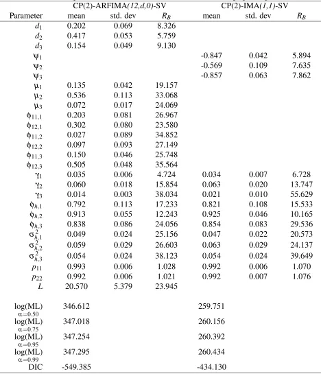
Table 9: Full sample estimation results for US core inflation, change-point specifications CP(2)-ARFIMA(12,d,0)-SV CP(2)-IMA(1,1)-SV Parameter mean std. dev RB mean std. dev RB

d1 0.202 0.069 8.326

d2 0.417 0.053 5.759

d3 0.154 0.049 9.130

ψ1 -0.847 0.042 5.894

ψ2 -0.569 0.109 7.635

ψ3 -0.857 0.063 7.862

µ1 0.135 0.042 19.157 µ2 0.536 0.113 33.068 µ3 0.072 0.017 24.069 φ11,1 0.203 0.081 26.967 φ12,1 0.302 0.080 23.580 φ11,2 0.027 0.089 34.852 φ12,2 0.097 0.093 27.149 φ11,3 0.150 0.046 25.748 φ12,3 0.505 0.048 35.564

γ1 0.035 0.006 4.724 0.034 0.007 6.728

γ2 0.060 0.018 15.854 0.063 0.020 13.747 γ3 0.014 0.003 38.034 0.021 0.010 55.629 φh,1 0.792 0.113 17.233 0.821 0.108 15.533 φh,2 0.913 0.055 12.243 0.925 0.046 10.165 φ_h,3 0.838 0.086 24.056 0.854 0.083 29.536

σ2

h,1 0.049 0.024 25.156 0.047 0.022 20.573 σ2

h,2 0.059 0.029 26.603 0.063 0.029 24.137 σ2

h,3 0.054 0.024 38.123 0.054 0.024 39.649

p11 0.993 0.006 1.028 0.992 0.006 1.070

p22 0.992 0.006 1.021 0.992 0.007 1.076

L 20.570 5.379 23.945

log(ML)

α=0.50

346.612 259.751

log(ML)

α=0.75

347.018 260.156

log(ML)

α=0.95

347.254 260.392

log(ML)

α=0.99

347.295 260.434

DIC -549.385 -434.130

Finally, we follow section 4.2 and assume that γk,σ_h2_,k ∼ IG 4₂,0₂.2

, φh,k ∼Beta(20,1.5), k =

1, ...,m, and pkk ∼Beta(20,0.1), k=1, ...,m−1. In this setting, the prior for each element ofθk

is very standard, while the prior for pkk favors infrequent structural breaks. In the appendix we

evaluate sensitivity of the results to different prior specifications by investigating alternative prior hyperparameter values on pkk.

We also report results for a change-point integrated moving average (IMA) model of order 1

with SV effects, CP(m)-IMA(1,1)-SV. This model corresponds to a CP(m)-ARFIMA(0,1,1)-SV model foryt or a CP(m)-ARIMA(0,0,1)-SV model for△yt. In this model changes in the long run

persistence are captured by changes in the MA(1) parameter,ψst3. We estimate CP(m)-IMA(1,1)

-SV from 0 to 4 change points and choose the optimal number of change points using ML and

DIC. Again, results point that the specification with 2 change points fits the data best. We report

estimation results for IMA(1,1) -SV and CP(2)-IMA(1,1)-SV in Tables 8 and 9.

We find that specifications with change points dominate the ARFIMA(12,d,0)model, both in terms of ML and DIC. Furthermore, compared to ARFIMA(12,d,0)-SV, the logBF in favor of CP(2)-ARFIMA(12,d,0)-SV is 75. For the ARFIMA(12,d,0)model the order of integration,d1,is

estimated at 0.38. This implies that US core inflation exhibits long memory behavior.φ12,1captures

the main seasonal effects. The average inflation rate, µ1 is estimated at 0.17%. Furthermore, the

residual standard deviation of the ARFIMA(12,d,0)model, σ1 is at 0.18% per month. When we

compare ARFIMA(12,d,0)with ARFIMA(12,d,0)-SV we find thatd1drops from 0.38 to 0.29. The

AR coefficients, φ11,1 and φ12,1 increase from 0.11 and 0.24 to 0.14 and 0.36 respectively. The

estimate ofµ1is also affected, being more precisely estimated at a lower value. The SV component

itself is nearly nonstationary as the autoregressive coefficient of volatility, φ_h,1, is close to one and

σ2

h,1, is well identified at 0.03 with a standard error of 0.01. The average variance of inflation,γ1is

estimated at 0.025% per month.

Figure 6 displays the data, estimates ofσ2

t =γstexp(ht), t=1, ...,T and the posterior density

of the change-point dates for CP(2)-ARFIMA(12,d,0)-SV. The posterior mode of the change-point density is associated with 1973:7 and 1984:2. Furthermore, from the top right panel of Figure 6 we

see that the volatility decrease in the early 1980s is noticeable and persistent. This phenomenon is

often labeled as “The Great Moderation”, see for example Stock and Watson (2007).

Overall, results from (4.6)-(4.7) conditional on 2 change points show that we can divide the

evolution ofyt into three subsequent phases: the period from 1960:1-1973:6, 1973:7-1984:1 and

1984:2 to the end of the sample. Both dst and µst are much smaller after the last change point,

d2=0.41 versusd3=0.15 and µ2=0.53 versus µ3=0.07. On the other hand, φ11,st andφ12,st

increase from 0.02 and 0.09 to 0.15 and 0.50 respectively. At the same time, the estimate of γst

almost doubles in the second regime while on the other hand it falls from 0.06 to 0.01 after the last

structural break. Furthermore, the unconditional volatility of volatility, σ_h,st/q1−φ2

st rises from

0.36 in the first regime to 0.60 in the second regime and falls to 0.42 from the last change point to

the end of the sample.

The last two columns of Table 9 report results for CP(2)-IMA(1,1)-SV. The estimate of ψ1,st

rises from −0.84 in the first phase to −0.56 in the second phase and drops to −0.85 in the

sub-sequent phase. Furthermore, similar to CP(2)-ARFIMA(12,d,0)-SV the unconditional volatility of volatility drops from the last change point to the end of the sample. However, CP(2)-IMA(1,1)-SV performs worse both in terms of ML and DIC compared CP(2)-ARFIMA(12,d,0)-SV.

To summarize: we find evidence of structural breaks in the dynamics ofyt. As expected, most

significant changes in the model parameters occur during the Great Moderation. More importantly,

it is also cautiously evident that the long memory characteristics of US inflation might have not

remained significant after the Great Moderation, as indicated by the lower persistence estimate for

the last regime, d3. We seem to agree with Stock and Watson (2007) that US inflation may have

become harder to model and forecast as the month-to-month memory has dropped.

[Figure6 about here]

We follow section 4.1 and compare the out-of-sample performance of CP(2)-ARFIMA(12,d,0) -SV (break) with ARFIMA(12,d,0)-SV (no-break). Specifically, we compare the out-of-sample predictive likelihood (PL) and predictive mean between these two models.

Given the data up to timet−1, Yt−1, the predictive likelihood (PL), p(yt, ..,yT |Yt−1) is the

predictive density evaluated at the realized outcome,yt, ...,yT,t≤T, see Geweke (2005). The PL

for modelM_{A is given as}

p(yt, ..,yT |Yt−1,MA) =

ˆ

ΘA

p(yt, ..,yT |θA,Yt−1,MA)p(θA|Yt−1,MA)dθA

=

T

∏

s=t

N−1

N

∑

i=1

p

ys|θ( i)

A ,Ys−1,MA

(4.8)

Notice that the terms on the right-hand-side of (4.8) have parameter uncertainty integrated out. If

t =1 this would be the marginal likelihood and (4.8) changes to (2.6). Hence, the sum of log predictive likelihoods can be interpreted as a measure similar to the log of the marginal likelihood,

but ignoring the initialt−1 observations.

The predictive likelihood can be used to order models according to their predictive abilities.

In a similar fashion to Bayes factors, one can also compare the performance of models based on

a specific out-of-sample period by predictive Bayes factors, PBF. The PBF for model A versusB

is given as PBFAB = p(yt, ...,yT |Yt−1,MA)/p(yt, ...,yT |Yt−1,MB) and summarizes the relative