International Doctorate School in Information and Communication Technologies
DISI - University of Trento
Statistical and relational learning for
understanding enzyme function
Elisa Cilia
Advisor:
Prof. Andrea Passerini
Universit`a degli Studi di Trento
Unravelling the functioning of the complex processes involved in living
systems is a challenging task. Enzymes are involved in almost all of the
chemical processes taking place within the cell. They accelerate chemical
reactions by forming a complex with the substrate and therefore lowering
the reaction activation energy. The characterisation of the enzyme function
at the molecular level is a fundamental step, which has several implications
and applications in modern biotechnologies. This thesis investigates
sta-tistical and relational learning techniques for the characterisation of the
enzyme function. The problem is tackled from two sides: the analysis of
the enzyme structure and its interactions with other molecules, and the
mining of relevant features from the enzyme mutation data. From the first
side a pure statistical learning approach is proposed for directly predicting
enzyme functional residues. This approach is shown to improve over the
current state of the art on several benchmark datasets. The engineered
predictors resulting from this investigation are now available to the public
of researchers through the CatANalyst web server. Further improvement
of the approach is pursued by proposing a supervised clustering technique
for collectively predicting all the residues belonging to the same functional
site. On the “learning from mutations” side, the focus shifts to the
ex-pressivity and interpretability of the learnt models. This thesis proposes
novel statistical relational approaches for mining hierarchical features for
multiple related tasks. The resistance of viral enzyme mutants to groups
of related inhibitors is modelled in a multitask setting. Learnt models are
improvements over both single and multitask alternatives. Moreover it has
the ability to provide explanation of the models which are themselves
hi-erarchical. A task clustering approach is also proposed for inferring the
structure of tasks when it is unknown. Finally, a relational approach is
proposed for exploiting the learnt relational rules for generating novel
mu-tations with specific characteristics. This allows to drastically reduce the
space of possible mutations to be experimentally assessed. Promising
pre-liminary results are obtained, which highlight the potential of the approach
in guiding mutant engineering and in predicting the viral enzyme evolution.
These findings can pave the way to further research directions in functional
interpretation of biological data by means of machine learning techniques.
Keywords
I really wish to thank
first of all, my advisor Andrea Passerini, for guiding me throughout this
joint work, advising me in every circumstance, being for me a scientific
reference point for both machine learning and bioinformatics aspects,
in-troducing me to the world of relational and statistical relational learning,
giving me examples of intellectual honesty and of how scientific work is
meant to be done, with his fresh and genuine commitment to research, and
much more;
Mauro Brunato, for the scientific support in the early stages of the work
and his unfailing friendship support along these four years, together with
his family;
Sergio Ammendola, for introducing me to the world of protein
bioin-formatics and the protein functional characterisation, and for the fruitful
collaborations that conferred further biological relevance to this thesis;
Niels Landwehr, for the precious collaboration in the development of the
hierarchical extension to kFOIL;
Franco Mascia, not only for the scientific collaboration and bizarre
dis-cussions in research related issues but especially for everything else;
Alessandro Moschitti, for initiating me into the world of machine
learn-ing and for the precious collaboration;
the members of the thesis commission, who helped me in improving the
PhD dissertation with invaluably helpful comments;
the unknown journal and conferences reviewers, who contributed in the
in schools and courses during my PhD: Anna Tramontano, Alex Smola,
Berhnard Sch¨olkopf and Nello Cristianini;
friends, people gravitating the Learning and Intelligent Optimization
group during this PhD course, and bioinformaticians at the Foundation
Edmund Mach for the support in the last months of preparation of the
PhD dissertation;
my family and my sister, far away from me in these years, to whom this
1 Introduction 1
1.1 Motivations . . . 2
1.2 The Protein Function Identification Problem . . . 9
1.2.1 Quick Primer on the Biological Aspects . . . 9
1.2.2 Defining a Protein Function . . . 13
1.3 Traditional Approaches to Protein Function Identification . 17 1.4 Review on Machine Learning Techniques . . . 19
1.4.1 Learning Paradigms and Learning Tasks . . . 19
1.4.2 Primer on Support Vector and Kernel Machines . . 23
1.4.3 Primer on ILP and Statistical Relational Learning . 31 1.4.4 Measuring and Comparing the Performance of Learn-ing Algorithms . . . 36
1.5 Aspects of Innovation . . . 37
1.6 Structure of the Thesis . . . 41
I Functional Residue Prediction 43 2 Identifying Functionally Important Residues 45 2.1 Introduction and Background . . . 45
3.1 The Learning Task . . . 58
3.2 Engineering Residue Features . . . 58
3.2.1 Features Extracted from the Sequence . . . 58
3.2.2 Modelling a Residue Structural Neighbourhood . . 59
3.2.3 Features Extracted from the Structure . . . 62
3.3 Experimental Results . . . 68
3.3.1 Datasets . . . 68
3.3.2 Experimental Setting . . . 69
3.3.3 Results of Different Feature Sets . . . 70
3.3.4 Comparison with Other Methods . . . 77
3.4 Engineering Active Site Features: Kernels on Structures . . 80
3.4.1 3D Kernel on Shapes . . . 80
4 Toward a Collective Learning Approach 93 4.1 Problem Description and Formalisation . . . 94
4.2 Distance-based Supervised Clustering with Maximum-weight Cliques . . . 98
4.3 The Maximum-weight Clique Clustering Algorithm . . . . 99
4.4 Experimental Results . . . 103
4.4.1 Predicting Active Sites . . . 103
4.4.2 Predicting Geometry of Metal Binding Sites . . . . 106
5 CatANalyst - Catalytic Residue Predictor 109 5.1 CatANalyst Web Server Architecture . . . 109
5.1.1 The Elaboration Engine . . . 111
5.2 Querying CatANalyst . . . 112
5.2.1 Job Submission . . . 112
5.2.2 Job Elaboration . . . 114
5.4 Statistics . . . 118
5.5 Computational Time Issues . . . 118
5.6 Work In Progress . . . 119
II Mining Relevant Features from Mutation Data 121 6 Learning from Mutations 123 6.1 Introduction and Background . . . 123
6.2 State of the Art . . . 130
7 Hierarchical Multitask kFOIL 133 7.1 Introduction . . . 134
7.2 kFOIL: Learning Relational Kernels . . . 135
7.2.1 The kFOIL Algorithm . . . 135
7.2.2 Multitask kFOIL . . . 140
7.3 Hierarchical kFOIL . . . 141
7.4 Task Clustering . . . 143
7.5 Experimental Evaluation . . . 146
7.5.1 Predicting Drug-Resistance of Mutants . . . 147
7.5.2 Protein Structure Classification . . . 159
8 A Relational Learning Approach Toward Protein Engineer-ing 167 8.1 Algorithm Overview . . . 169
8.1.1 Background Knowledge . . . 169
8.1.2 The Approach . . . 171
8.2 Experimental Evaluation . . . 174
8.3 Discussion . . . 177
8.4 Future Work . . . 179
9 Conclusions 183
1.1 Growth of UniprotKB released sequences. . . 4
1.2 Growth of PDB released protein structures per year. . . . 5
1.3 The Central Dogma of molecular biology. . . 10
1.4 Amino acid. . . 11
1.5 Peptide bond formation. . . 13
1.6 Structure of an α-helix and a β-sheet. . . 13
1.7 The levels of a protein structure . . . 14
1.8 Enzyme Classification number. . . 16
1.9 Pie chart of the results of the “enzyme” query to the Unipro-tKB. . . 17
1.10 Supervised learning. . . 21
1.11 Soft margin SVM. . . 27
1.12 Mapping in a new feature space. . . 28
2.1 Active site schematisation. . . 47
2.2 Roles of metal ions in enzymes. . . 49
2.3 Three different proposed approaches for active site identifi-cation. . . 50
3.1 A residue 3D representation. . . 60
3.2 The L-arginine:glycine amidinotransferase (1JDW) and its highlighted catalytic pocket. . . 61
neighbourhood of a catalytic residue. . . 83
3.5 Histogram of the frequencies of heterogen molecules in the
PW dataset. . . 84
3.6 Histograms of the distances of the most frequent heterogens
from catalytic residues in the PW dataset. . . 85
3.7 Vector of the feature weights w~ of a classifier trained on the
PW dataset. . . 86
3.8 ROC and Recall/Precision curves . . . 87
3.9 Local ROC curves of the predictions on different
benchmark-ing datasets . . . 88
3.10 Global ROC curves of the predictions on different
bench-marking datasets . . . 89
3.11 Recall/Precision curves of the predictions on different
bench-marking datasets . . . 90
3.12 ROC curves superimposed with those reported in [134] on
the PW dataset. . . 91
3.13 Two examples of triangular shapes extracted from the HYS303 three-dimensional neighbourhood. . . 91
4.1 Histogram of the catalytic propensities of the residues in the
experimental dataset HA superfamily . . . 95
4.2 Metal binding sites in the sequence of the equine herpes
virus-1. . . 96
4.3 Functional residues in the sequence of the cloroperoxidase T. 97
5.1 CatANalyst web server architecture. . . 110
5.2 Input form for the sequence-based CatANalyst prediction. 113
5.3 Input form for the structure-based CatANalyst prediction. 114
5.6 Results of experiments for the CatANalyst online predictors 117
6.1 Correlation plot of the prediction margins of the residues in
the wild type enzyme (x axis) and one of its mutants (y axis).125
6.2 Portion of the predicted 3D model of SsAH including the
active site. . . 126
6.3 Reverse transcriptase inhibition by Nevirapine (PDB code 1VRT). . . 128
7.1 Example of a relational kernel function for the HIV resis-tance mutation database. . . 138
7.2 The hierarchical learning approach. . . 141
7.3 Example hierarchy of learnt clauses. . . 153
7.4 Hierarchical clustering dendrograms. . . 156
7.5 Relative frequency of the background knowledge predicates in the learnt models. . . 163
7.6 Example of EF-hand like protein structure. . . 165
8.1 Schema of the mutation engineering algorithm. . . 172
8.2 Example of learnt hypothesis for the NCRTI task with high-lighted mutations covered by the hypothesis clauses. . . 173
8.3 Mean recall by varying the number of generated mutations. 178 8.4 Detail of the mean recall curves of the NNRTI task for a number of generated mutations below 150. . . 179
8.5 Example of application of the approach for mutant engineer-ing. . . 181
In this thesis some of the molecular graphics images or parts of them were produced using the UCSF Chimera package [112] from the Resource
Cal-1.1 Amino acid alphabets. . . 12
3.1 Sequence-based Features Representation: features extracted
from the protein sequence . . . 58
3.2 Structured-based Features Representation: scalar features
extracted from the residue structural neighbourhood. . . . 63
3.3 Classification of the heterogens into three groups. . . 67
3.4 Legend of abbreviations for the different sets of attributes . 70
3.5 Heterogen Analysis . . . 72
3.6 Statistical analysis . . . 73
3.7 Comparison with state-of-the-art sequence-based approach [151] 77
3.8 Comparison with structure-based approaches by Chea et al.
[37] and Youn et al. [149] . . . 78
3.9 Comparison with structure-based approach by Tang et al. . 79
3.10 Comparison with the POOL structure-based approach . . . 80
4.1 Comparison of the results obtained in active site prediction
with the distance-based supervised learning approach . . . 105
4.2 Comparison on the metalloproteins dataset . . . 108
4.3 Experimental results on the metalloproteins dataset . . . . 108
5.1 CatANalyst’s scheduler policy and job queues. . . 111
datasets with associated number of instances. . . 149
7.2 Summary of the HIV drug resistance background knowledge
facts and rules. . . 149 7.3 Amino acid types encoded in colour classes. . . 150 7.4 Summary of the hierarchical multitask experiments . . . . 152
7.5 Summary of the hierarchical clustering experiments . . . . 158 7.6 Number of examples (N) in each of the folds in the SCOP
dataset. . . 160
7.7 Summary of the SCOP background knowledge. . . 161 7.8 Summary of the hierarchical multitask experiments for the
SCOP dataset. . . 162
8.1 Summary of the background knowledge facts and rules. . . 170
8.2 Statistical comparisons of the performance of the algorithm
4.1 WMC main procedure. . . 101
4.2 The ChooseNode procedure. . . 103
7.1 kFOIL algorithm. . . 137
7.2 Hierarchical kFOIL algorithm. . . 142
7.3 kFOIL refinement algorithm. . . 143
7.4 Hierarchical clustering kFOIL algorithm. . . 146
7.5 kFOIL algorithm for cluster node. . . 146
Introduction
The beginning of the genomic era made it possible for scientists to compare the genome sequences of different organisms and species. These genome se-quences can have different size and complexities depending on the organism they belong to, from viruses and bacteria, to plants and mammals.
The availability of the human genome sequence has emphasised how far we still are from understanding the relationship between the structure of
the molecules and their function.
By analysing the human genome and genomes of simpler organisms
re-searchers observed that the number of genes is not proportional to the size or the complexity of an organism. This observation led to the paradox that, for instance, the human genome contains some tens of thousands
of genes [110], encoding approximately the same number of well charac-terised proteins, but apparently, the number of protein functions seems to be higher. This sort of paradox can be explained by hypothesising that one gene codes for more than one protein (an example is given by the
al-ternative splicing mechanism) and that the same protein is able to perform more than one function. Hence, identifying the function or the functions that a protein performs is one of the big challenges characterising the
Small variations of the same protein can be present within different organs of the same organism and between different species. This makes
the protein function identification still more challenging and the analysis and mining of such a large quantity of biological data requires the use of automated approaches.
Computational methods can play a key role in “omics” projects aiming
at giving a functional interpretation to the information contained in the genomes. The birth of a discipline like bioinformatics is the evidence of the importance of computational approaches in genomics and proteomics
projects.
1.1
Motivations
The goal of protein bioinformatics is to assist experimental
bi-ology in assigning a function or suggesting functional hypothesis
for all known proteins. The task is formidable. A simple
calcula-tion shows that we cannot possibly study each and every
biologi-cal molecule of the universe. Therefore, we need fast and reliable
computational methods to extrapolate the knowledge accumulated
on a subset of cases to the rest of the protein universe.
Anna Tramontano in “The Ten Most Wanted Solutions in Protein Bioinformatics”
Bioinformatics is a recently born discipline. Its aim is to analyse the information contained in the biological molecules — nucleic acids and pro-teins — by means of computational methods. Past research in bioinfor-matics has been devoted to the production and understanding of genomic
data, but recently it is increasingly permeating other fields of biology like functional and structural genomics and proteomics.
Protein bioinformatics has the main objective to discover the
pathologies, which lead to an altered or null protein function. Through the knowledge of these mechanisms it is possible to understand the complex processes involved in living systems and possibly correct dysfunctional
be-haviours. Such research is quite complex to carry out as a protein function involves a combination of several factors, many of which are still unknown.
Knowing the protein three-dimensional structure is of primary impor-tance for understanding its role and its function. The three-dimensional shape allows the protein to correctly interact with other molecules and
macromolecules. The function that the protein carries out varies on the basis of the spatial conformation it assumes. The three-dimensional struc-ture of a protein can be experimentally determined. Two quite expensive techniques are used with this aim: the X-ray crystallography [53] and the
Nuclear Magnetic Resonance (NMR) [144].
Large scale genomics projects [81] are providing a huge amount of
pro-tein sequential and, at a lower but increasing rate, structural informa-tion [24, 27]. At the beginning of november 2010 the Universal Protein Re-source database (UniprotKB) [131] counted for more than twelve millions
of synthesised proteins. Figure 1.1 shows the growth of the database in the last years for the manually annotated and reviewed sequences (Swiss-Prot) and the automatically annotated and not reviewed sequences (TrEMBL).
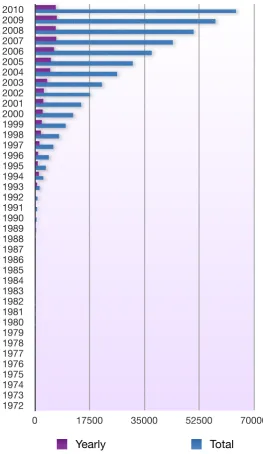
At the same date, the database of protein structures, Protein Data Bank (PDB) [14], maintained by the Research Collaboratory for
Struc-tural Bioinformatics (RCSB), reported more than 64000 deposited protein structures. A large portion of such proteins have their function still un-determined, as it is often not straightforward to understand the details of a protein function even when its three-dimensional structure is known.
(a) Growth of UniprotKB/Swiss-Prot released sequences.
(b) Growth of UniprotKB/TrEMBL released sequences.
Figure 1.1: Growth of UniprotKB released sequences.
Considering the rate at which protein sequences are synthesised and
in narrowing this gap.
Number of searchable structures per year. Number of searchable structures per year. Number of searchable structures per year.
Note: searchable structures vary over time as some become obsolete and are removed from the database. Note: searchable structures vary over time as some become obsolete and are removed from the database. Note: searchable structures vary over time as some become obsolete and are removed from the database. Year Yearly Total
2010 6591 64201
2009 6969 57610
2008 6577 50641
2007 6809 44064
2006 6059 37255
2005 5021 31196
2004 4832 26175
2003 3835 21343
2002 2770 17508
2001 2598 14738
2000 2391 12140
1999 2116 9749
1998 1842 7633
1997 1372 5791
1996 964 4419
1995 851 3455
1994 1201 2604
1993 631 1403
1992 156 772
1991 167 616
1990 132 449
1989 61 317
1988 50 256
1987 18 206
1986 16 188
1985 18 172
1984 21 154
1983 34 133
1982 28 99
1981 14 71
1980 6 57
1979 10 51
1978 4 41
1977 24 37
1976 13 13
1975 0 0
1974 0 0
1973 0 0
1972 0 0
2010 2009 2008 2007 2006 2005 2004 2003 2002 2001 2000 1999 1998 1997 1996 1995 1994 1993 1992 1991 1990 1989 1988 1987 1986 1985 1984 1983 1982 1981 1980 1979 1978 1977 1976 1975 1974 1973 1972
0 17500 35000 52500 70000
Yearly Total
Figure 1.2: Growth of PDB released protein structures per year.
The most used approaches for the functional characterisation of genes
exploiting the sequence and structural comparison of new proteins with manually annotated ones, it is possible to assign a function to a large number of proteins in a fraction of the time and cost needed for a
lab-oratory study. Unfortunately those simple approaches have shown their limitations in various context (see Section 1.3). Furthermore, an anno-tated homologue of the target protein needs to be available preventing the homology transfer applicability to novel folds and the increasing lack of
functional annotations makes this strategy even less effective.
Machine learning techniques provided a valid alternative to homology-based methods. They allow for the development of predictors that are able to abstract from the single case and learn an accurate statistical or logical model based on known examples (supervised learning).
In this thesis the focus is on the characterisation of the molecular func-tion of enzymes. Enzymes are those proteins whose role is to accelerate
chemical processes inside a cell. The identification of the enzyme function is a required step for the innovation of biotechnologies used in the agri-culture and food fields, as well as in the pharmacological and biochemical
fields. New enzymes can be produced for their application in agriculture and food biotechnological processes as, for instance, enzymatic sensors for food control, or in water depuration and soil treatment and disinfection. From the pharmacological side, understanding the mechanisms of enzymes
operation is fundamental for making an antibiotic an effective drug. En-zymes present in pathogenic bacteria must be able to form a complex and therefore to inhibit proteins that are essential for the bacterium life.
An enzyme function is defined by a topological region — called func-tional or active site — composed of amino acid residues located in specific
proper-ties. The second is to characterise the properties of the single amino acids involved and the way in which they interact among each other and with other molecules, e.g. drugs.
Two “wet laboratory” approaches are typically used for gaining insights
about an enzyme molecular function: inhibition studies and random mu-tagenesis. By inhibiting one amino acid at a time and then by observing variations in the enzyme activity it is possible to infer a putative functional
role of the inhibited residues. In principle, the inhibition of a functional residue should correspond to a decrease and sometimes to a complete loss of the enzyme biological activity. Random mutagenesis aims at generating a number of mutants of the same enzyme (the wild type). While directed
mutagenesis requires the knowledge of the sequence or the structure of the protein, random mutagenesis can be applied without knowing any informa-tion and allows for the creainforma-tion of a library of mutants to be screened. The induced mutations can lead to inactive mutants, more convenient mutants
showing an improved biological activity or, they can be neutral mutations not affecting the enzyme activity. By analysing the common patterns of mutation and their correlation with the observed mutant activity it is
pos-sible to formulate hypotheses on the functional sites and the amino acids involved in them.
The analysis and mining of information from mutation data is also ex-tremely important in molecular genetics studies aiming at developing
ef-fective cures to a number of diseases that stem from specific protein de-fects [143]. Diseases like the cystic fibrosis, cancer and Human Immunode-ficiency Virus (HIV) infection all depend in some way on specific mutations taking place into specific proteins, especially enzymes — for the cystic
understand these many aspects. The virus has a high mutation rate and it is prone to the development of the resistance to specific drugs. Hence, the analysis of the virus mutations and the discovery of those residues that
are necessary for the virus proteins proper functioning, is extremely impor-tant. Moreover, drug resistance development is often the result of multiple mutations occurring along the primary sequence. The correlation among mutations and their relationship with the resistance to a drug should be
also taken into consideration.
Geometrical and statistical approaches are crucial for understanding the relationship between molecular structures and their function. Geometrical approaches are needed for managing and analysing structural properties of the molecules and their interactions. Statistical approaches are needed
for handling and analysing large quantity of data, with the aim of ex-trapolating rules that can be generalised to novel cases. In particular, machine learning techniques can be used for identifying spatial regions hosting protein binding and functional sites. They can also be very useful
in determining each one of the functional residues or reducing the number of candidates to be experimentally verified.
In the last years, the most promising machine learning techniques have evolved in the direction of learning from structured objects — such as sequences and graphs — and performing structured prediction. Among
the supervised learning techniques, kernel methods [123] and especially Support Vector Machines (SVMs) [23, 43] have been successfully applied to several bioinformatics applications [76].
Statistical Relational Learning (SRL) [64] techniques also shown to be particularly suitable for learning and mining data in bioinformatics
the robustness principles of the statistical learning theory.
The aim of this thesis is to investigate and develop effective and
ad-vanced machine learning techniques for helping in characterising enzyme molecular functions and understanding the mechanisms allowing the pro-teins to operate. For instance, machine learning approaches for mining features that are relevant for causing the enzyme functioning or the
en-zyme malfunction, can be very useful. They can suggest the reason why a mutant shows an improved or reduced activity on a certain drug or, why an enzyme is resistant to a certain drug and/or not resistant to another
one. For instance, by modelling the presence of a mutation close to the functional site that changes a structural amino acid, like a proline, into a large and basic amino acid, like arginine or lysine.
1.2
The Protein Function Identification Problem
In the previous section the problem of the protein function understanding and its complexity has been introduced, but what is a protein and how can
we define its function?
In this section a short introduction to the underlying biological aspects needed to understand the rest of the work will be given.
1.2.1 Quick Primer on the Biological Aspects
The complex processes involved in living systems are the result of the
harmonic action of molecules and macromolecules, mainly proteins. The cell is a complex biochemical machinery and proteins are its “functional devices”.
DNA to RNA to protein” (Figure 1.3).
DNA RNA Protein
duplication transcription translation
Figure 1.3: The Central Dogma of molecular biology.
Each gene in a cell genome is a deoxyribonucleic acid (DNA) fragment, which codes for a protein. Hence, genes “building blocks” are nucleotides,
made of the union of a sugar (deoxyribose) and one of the four bases: adenine (A), guanine (G), cytosine (C), and thymine (T). The sequence in which the nucleotides are placed along the DNA strand determines the
properties of the different genes.
Each one of the triplets of a gene sequence in the alphabet ΣN =
{A, C, T, G} codes for one of the twenty amino acid in nature, in the
al-phabet
ΣP = {A, C, D, E, F, G, H, I, K, L, M, N, P, Q, R, S, T, V, W, Y},
according to the universally accepted Genetic Code [106].
Amino acids are the “building blocks” of proteins. They are organic
molecules characterised by two functional groups: an aminic group (N H2) and an acidic group, the carboxylic group (COOH), which together give the name of “amino acid”.
The two functional groups are held together by a carbon atom, known as alpha carbon (Cα). A further chain of atoms, bound to the Cα, makes the amino acid side-chain (R), which differentiates from the main chain
hydrogen atom, as in the case of a glycine, to more complex structures of benzene rings, as for a tyrosine.
H N C C OH
H
R H
side-chain
main-chain carboxylic group amino group
alpha carbon
O
Monday, 22 March 2010
Figure 1.4: Amino acid.
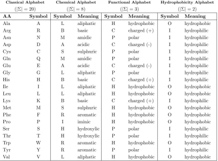
Table 1.2.1 also shows the classical 20 symbol alphabet with the three-letter and the corresponding one-three-letter abbreviations for the amino acids. Since the twenty amino acids differ on the basis of the chemical properties
of their side chain (which can be polar, apolar, acid or basic), different al-phabets can be used that group them according to functional and chemical properties (see Table 1.2.1).
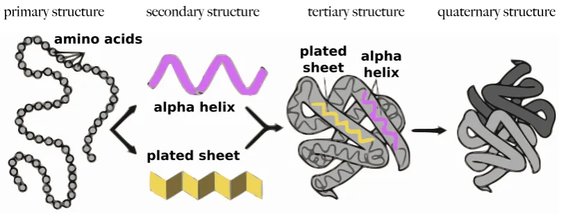
A protein is composed of one or more chains of amino acids held together by a peptide bond, a covalent bond between the carboxylic and the amino group of two consecutive amino acids. The formation of a peptide bond
between to amino acids (see Figure 1.5) produces a free water molecule.
The result is a polypeptide chain of residues of amino acids. The se-quence of the residues along the chain is the proteinprimary structure. The
amino acids along the chain, due to their three-dimensional structure, can arrange into often repetitive and bound structures, called secondary struc-ture elements (SSE), for example β-sheets and α-helices (see Figure 1.6). The tertiary structure, is the result of the chain folding process, due to:
Classical Alphabet Chemical Alphabet Functional Alphabet Hydrophobicity Alphabet
(|Σ|= 20) (|Σ|= 8) (|Σ|= 3) (|Σ|= 2)
AA Symbol Symbol Meaning Symbol Meaning Symbol Meaning
Ala A L aliphatic H hydrophobic O hydrophobic
Arg R B basic C charged (+) I hydrophilic
Asn N M amidic P polar I hydrophilic
Asp D A acidic C charged (-) I hydrophilic
Cys C S sulphuric P polar I hydrophilic
Gln Q M amidic P polar I hydrophilic
Glu E A acidic C charged (-) I hydrophilic
Gly G L aliphatic P polar I hydrophilic
His H B basic C charged (+) I hydrophilic
Ile I L aliphatic H hydrophobic O hydrophobic
Leu L L aliphatic H hydrophobic O hydrophobic
Lys K B basic C charged (+) I hydrophilic
Met M S sulphuric H hydrophobic O hydrophobic
Phe F R aromatic H hydrophobic O hydrophobic
Pro P I iminic H hydrophobic O hydrophobic
Ser S H hydroxylic P polar I hydrophilic
Thr T H hydroxylic P polar I hydrophilic
Trp W R aromatic H hydrophobic O hydrophobic
Tyr Y R aromatic P polar I hydrophilic
Val V L aliphatic H hydrophobic O hydrophobic
Table 1.1: Amino acid alphabets.
H N C C OH H
R
H O
H N C C OH H
R
H O
H N C C
H
R
H O
N C C OH
H
R
H O
O
H H
Monday, 22 March 2010
Figure 1.6: Structure of an α-helix and a β-sheet.
chain is dip into. Finally the quaternary structure is the composition of
a number of polypeptide chains belonging to the same protein, in other words, it is the whole set of subunits that compose an oligomer. The four levels of a protein structure are visualised in Figure 1.7.
Figure 1.7: The levels of a protein structure (adapted from a courtesy of the National
1.2.2 Defining a Protein Function
There is no single or fully standardised way of defining a protein function.
A protein function can be defined at the molecular, biological or cellular scale and, at each level, further levels of detail can be considered. Further-more, a protein function has many other distinctive aspects that depend on
the environment in which the protein operates and which conditions affects its behaviour [61]. For example, the same enzyme can perform different functions depending on whether it is located in the liver or in the eye.
Proteins inside the cell perform several different functions. Three fun-damental examples are storage proteins, structural proteins and enzymes. At the biological level we can distinguish among enzymes, transport pro-teins (haemoglobin), hormones and propro-teins involved in defence against
germs (antibodies), in structural support or body movement (contractile proteins) [143].
A quite successful attempt to standardise the protein function definition
at the different scales is represented by the Gene Ontology (GO) [29]. Concepts in the GO, called GO terms, are organised in a directed acyclic graph (DAG) structure. GO terms are connected on the base of a general-to-specific relation.
This thesis focuses on one of the aspects of a protein function definition: the molecular function. At the molecular level a protein function is defined by a topological region of the protein called functional site, which is a
functional domain in the protein three-dimensional structure. Functional domains can have a multiplicity of roles within a protein. For example in enzymes, functional domains are also called active or catalytic sites, while
in other kind of proteins they correspond to binding sites with another macromolecule.
proteins able to accelerate chemical processes inside a cell. The enzyme works by forming complexes with the reactants and in doing so it lowers the activation energy of the reactions thus increasing their rate. This process is
the catalysis. An enzyme has usually the structure of a globular protein and the 3D disposition of the residue chain is somewhat specific. The residues take up well-defined positions which are essential for the recognition and binding of specific substrates, in other words, for the biological activity
of the enzyme. The residues that are directly involved in the catalytic process (e.g. nucleophiles, proton-donors) constitute the active site, while residues in the surrounding space play the role of attracting and orienting
the molecule to bind and constitute the binding domain.
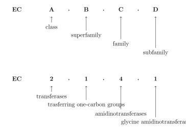
The Enzyme Commission (EC) Nomenclature, proposed by the Inter-national Union of Biochemists (IUB), is the first example of an enzyme molecular function categorisation. The classification has the aim to
stan-dardise the definition of the enzyme function by assigning reactions to a hierarchy of four categories from general to specific, namely the class, the superfamily, the family and the subfamily (Figure 1.8).
Enzymes are grouped in six functional classes in the EC Nomenclature,
based on the type of the catalysed reaction:
1. oxidoreductases, for oxidation-reduction reactions;
2. transferases, for the transfer of functional groups;
3. hydrolases, for hydrolysis reactions;
4. lyases, for breaking chemical bonds;
5. isomerases, for isomeration reactions;
EC A . B . C . D
class
superfamily
family
subfamily
EC 2 . 1 . 4 . 1
transferases
trasferring one-carbon groups
amidinotransferases
glycine amidinotransferase
Figure 1.8: Enzyme Classification number.
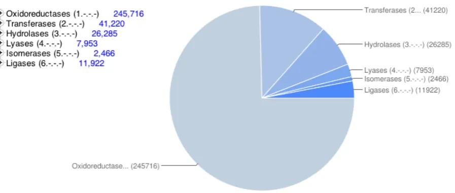
The pie chart in figure 1.9 shows the results obtained by querying the UniprotKB with the keyword “enzyme”. The chart highlights the number
of synthesised enzymes currently in the Uniprot divided by EC class.
In order to perform their function, many enzymes need to be bound to an additional non-protein component called cofactor. Cofactors can be
grouped in:
(a) coenzymes, i.e. dissociable cofactors that are usually organic;
(b) prosthetic groups, i.e. non dissociable cofactors.
Figure 1.9: Pie chart of the results of the “enzyme” query to the UniprotKB.
1.3
Traditional Approaches to Protein Function
Iden-tification
Traditional approaches for the functional characterisation of genes and
their proteins implement homology-based strategies. Novel protein func-tion is inferred by aligning the sequences or by superimposing the structures with already annotated proteins and then by transferring the annotation
from the most similar to the novel one.
Typically, sequence databases are searched for finding a significant se-quence similarity to another protein whose function has been experimen-tally characterised. Basic Local Alignment Search Tool (BLAST) [28] is a
popular tool for searching a query sequence against a database of known protein sequences and discovering sequence similarities. For this reason the word “BLASTing” is often used nowadays referring to this search process.
The biological rationale for the homology-based transfer is as simple as
The protein structure is even more informative than the amino acid sequence alone. Knowing the protein structure is fundamental for under-standing the biochemical mechanisms by which the protein performs its
function. Whenever the tertiary structure of a novel protein with unknown function is available, the structural similarity to other proteins can allow the functional annotation transfer [61]. For instance, two protein struc-tures with the same fold can have an identical or similar function even if
the two protein sequences have little similarity [25]. That is because the protein tertiary structure tends to be more preserved than the primary structure along evolution.
By using automatic approaches exploiting the sequence and structural
similarity of new proteins with manually annotated ones, it is possible to assign a function to a large number of proteins in a fraction of the time and cost needed by a laboratory study [58]. Unfortunately those simple approaches have shown their unreliability for functional annotation
even in presence of a high sequence or structural identity percentage and other limitations in various context. First, an annotated homologue of the target protein needs to be available preventing their applicability to novel
folds. Furthermore, if a protein has more than one domain a detected evolutionary relationship, even based on a high sequence similarity with another protein, can be limited to only one of the domains, leading to an erroneous annotation [135]. Even considering the 3D structure similarity,
there are cases in which proteins with similar overall tertiary structure can have different active sites, i.e. different functions [101, 133], and proteins with different overall tertiary structure can show the same function and
similar active sites. Finally, the increasing lack of functional annotations makes the homology-based strategies even less effective as it becomes even more difficult to find an annotated reference sequence for novel proteins.
homology-based methods in cases in which the homology-homology-based transfer cannot be applied. These methods are able to abstract from the single case and to learn accurate statistical or logical models based on observations. In recent
years they have been successfully applied for predicting enzyme functional sites and functional residues.
1.4
Review on Machine Learning Techniques
Machine learning primary aim is to provide effective algorithms for training a machine in automatically acquiring useful and accurate models from the experience.
A plethora of machine learning algorithms have been proposed in re-cent years, with different peculiarities concerning the problem formalisa-tion they approach, the underlying method used, and how efficiently they are able to solve a learning task.
The following sections present a rapid excursus on the learning paradigms, tasks, and algorithms that are of interest for this thesis.
1.4.1 Learning Paradigms and Learning Tasks
Machine learning is a wide field that includes many different approaches for solving different learning problems: from medical diagnosis and financial
analysis, to speech recognition and text categorisation or image analysis and computer vision. In recent years these algorithms have been also suc-cessfully applied to solve several bioinformatics applications [88].
Supervised Learning
In supervised learning, we are given a set of examples (x(i), y(i)) ∈ X × Y with i = 1, ..., m, where X is the input space and Y is the output space. The learning problem is to derive a model h : X → Y for the unknown input-output relationship. This is achieved combining fitting of the training data with some constraints on the hypothesis space, in order to avoid overfitting and generalise to unseen instances. A typical approach consists of penalising overly complex hypotheses, a procedure
called “regularisation”.
The error in fitting training data is formalised as the empirical risk:
Emp[h(·) 6= y] = 1
m
m
X
i=1
l(y(i), h(x(i))) (1.1)
where l : Y × Y → R is a loss function, which returns values according to the “goodness” of the prediction h(x) with respect to the real output y. If we consider the 0-1 loss, which is defined as:
l(y,yˆ) =
0 if y 6= ˆy
1 otherwise
(1.2)
where ˆy = h(x), the empirical risk corresponds to the number of misclas-sified instances of the training set.
Figure 1.10, adapted from [129], schematises the learning supervised by examples. A new example x is assigned to y according to the learnt model
h.
Depending on the nature of the output space Y, we can distinguish
among different learning tasks. The most common are:
– binary classification whenever l = 2, typically Y = {+1,−1}
a new example is classified in one of two classes (as positive or negative);
– multiclass classification whenever l > 2.
• regression Y = R is a continuous set.
The rest of the thesis focuses on classification problems. Classification and regression are standard supervised learning problems in which the outputs are simple scalars. The output space Y can be also characterised by more complex and structured objects like, sequences, trees or graphs (see section
1.4.2).
HypothesisH
h:X 7→Y
Labeled data
(x(i), y(i))
Learning find h∈H
s.t. y(i) ≈h(x(i))
Prediction y=h(x)
new datum
x
Figure 1.10: Supervised learning (taken from [129]).
Multitask Learning [34] is a particular example of supervised learning
paradigm consisting in learning a model for a task and other related tasks at the same time. It deals with the problem of exploiting information on related tasks in order to improve the predictive performance and it is
considered a kind of inductive transfer.
In this setting given a set T of learning tasks and, for each t ∈ T, a set of examples Dt = {(x(
i) t , y
(i)
derive simultaneously a model ht for each t ∈ T such that ht(x( i)
t ) ≈ y
(i) t
while retaining the capability of the models to generalise to unseen data.
Indeed, the primary aim of multitask learning is to improve the generalisa-tion performance of a learnt model leveraging addigeneralisa-tional informageneralisa-tion from related tasks.
Unsupervised Learning
In unsupervised learning input data x(i) with i = 1, ..., m, have no super-vised target outputs. The objective is to learn how data are organised,
reveal patterns from them or build a representation that can be used for further analyses [65]. Clustering falls in this category.
Given a set D of m inputs, the problem is to find a set C ⊆ P(D) such that
C = {Cj ∈ P(D)|
[
j
Cj = D ∧
\
j
Cj = ∅}
Consequently a partial clustering can be defined as:
CP = {Cj ∈ P(D)|
[
j
Cj ⊆ D ∧
\
j
Cj = ∅}
The hierarchical clustering is a popular approach to clustering, which is
of interest in the present thesis. This clustering technique, differently from partitioning approaches, does not require to specify a priori the number of desired clusters. The algorithm can proceed with a bottom-up strategy,
by starting with singletons and recursively aggregating pair of clusters. Alternatively, a top-down strategy can be followed by splitting an initial cluster with all the examples recursively into smaller clusters. Merging or splitting two clusters require to define inter-cluster similarity or distance
measures (the linkage function).
dendro-gram, i.e. at different similarity thresholds, a different clustering — with different number of clusters — can be obtained.
The hierarchical clustering can provide noticeable additional informa-tion on the structure of the data.
1.4.2 Primer on Support Vector and Kernel Machines
Among the supervised learning techniques kernel methods [123] and espe-cially SVMs [23, 43] have been successfully applied to many problems in computational biology [124].
Some examples are translation initiation site recognition in DNA genes [152], promoter region-based classification of genes [109], protein-protein
interaction [20], functional classification from microarray expression data [108], protein function classification [21].
Support Vector Machines
SVMs are learning algorithms based on principles of the statistical learning theory [139]. They aim at linearly separating examples with a large margin, possibly accounting for margin errors [42].
Suppose that X = Rn, i.e. examples are represented as vectors of fea-tures, and that we can define an inner product h·,·i on X. An SVM learns the parameters of an hyperplane separating positive and negative
exam-ples. In Figure 1.11(a) examples of separating hyperplanes are shown. The functional margin γi of an example with respect to an hyperplane
hw, ~~ xi + b = 0 is the product yi(hw, ~~ xii + b). Its geometrical definition
that realises the maximum margin γ over the training set. Results from the statistical learning theory state that the h that grants the lowest bound on the generalisation error is the one that maximises the separation among
positive and negative examples.
! ! ! "#$%&'('!)*%+',! !!!!!!!!!!!!!!!!!!!!!!!!!!!!!!!!!!!!!!!!!!!!!!!!!!!!!!!!!!-.&*'/01%'.2! !"#$%&'#"#%& & () & *#+,-%&).)(/&0%-+#1#&2#&$34%-%5#613& & 7,3""6&23""%&-#83-8%&23"&9%$$#96&9%-+#13&:&,1&4-6;"39%&2#&6<<#9#55%5#613=&"%&8,#&
>,15#613& 6;#3<<#?6& 2%& 9%$$#9#55%-3& :& w k
& =& 861&3& 9%-+#13& 23""@#43-4#%16=&
$6<<646$<%&%#&?#186"#&Ji yi(w&x&ib)tk.&
& *#+,-%&).)A/&B43-4#%16&%&9%$$#96&9%-+#13&&
&
0
x b w& &
k b x w&&
k b x w&& w&
(a) Separating hyperplanes.
(b) Maximal separating hyperplane.
Finding the maximal margin hyperplane translates into solving the fol-lowing optimisation problem (hard margin):
minw,b~ 12||w||~ 2
subject to yi(hw, ~~ xi+b) ≥ 1 ∀i = 1, ..., m
(1.3)
where b ∈ R and w~ ∈ Rn. Note that, this primal formulation is obtained after a rescaling of w~ in a way that the points lying on hw, ~~ xi + b = ±γ
now lie on hw, ~~ xi+b = ±1.
This quadratic convex optimisation problem has a unique global
opti-mum. Given the learnt hyperplane, the decision function is simply:
h(~x) = sgn(hw, ~~ xi +b) (1.4)
separable training sets and more complex input data. By deriving the Langrangian of the primal optimisation problem in 1.3, we first obtain:
L(w, b, ~~ α) = 1 2||w||~
2 − m
X
i=1
αi(yi(hw, ~~ xi+b)−1) (1.5)
where αi ≥ 0 are the langrangian multipliers for incorporating the linear constraints. By differentiating the Langrangian with respect to the primal variables and setting the derivatives to be equal to 0, we obtain:
∂L(w, b, ~~ α)
∂ ~w = 0 ⇒ w~ =
m
X
i=1
αiyi~xi (1.6)
∂L(w, b, ~~ α)
∂b =
m
X
i=1
αiyi = 0 (1.7)
Substituting 1.6 and 1.7 in the primal Langrangian 1.5 we obtain the dual form of the optimisation problem 1.3:
maxα∈Rm
Pm
i=1αi − 12
Pm
i,j=1yiyjαiαjh~xi, ~xji
subject to αi ≥0 ∀i = 1, ..., m
Pm
i=1yiαi = 0
(1.8)
In this dual formulation training data appear only in the so called Gram
matrix, of their inner products. By substituting 1.6 in 1.4, the decision function becomes:
h(~x) = sgn( m
X
i=1
αiyih~xi, ~xi+b)
The Karush-Khun-Tucker conditions state that the optimal solution
α∗i(w~∗, b∗) satisfies the following relation:
This implies that if α∗i = 0, the training input ~xi is not affecting w~∗ other-wise yi(hw~∗, ~xii+ b∗)−1 must be equal to 0, hence ~xi lies on the frontier distant 1 from the maximal hyperplane. The latter points ~xi are thesupport
vectors and are the only ones of interest for characterising the separating function. In Figure 1.11(b) the support vectors and the maximum margin hyperplane are highlighted in orange.
Soft Margin SVM
With the aim of improving the generalisation and separability in case of noisy data, the primal optimisation problem 1.3 can be rewritten relaxing the constraints for taking into account classification errors. Regularisation
can be introduced in the objective function. The resulting optimisation problem is:
minw,b,ξ 12||w||2 + C
Pm
i=1ξi
subject to yi(hw, xi+b) ≥ 1−ξi ∀i = 1, ..., m
(1.10)
where ξi ≥ 0 are slack variables for constraints relaxation and C is the regularisation parameter that measures the tradeoff between the
misclas-sification error and the margin maximisation. As C grows, margin errors are more penalised. Therefore, for C → ∞ the problem approximates the solution with the hard margin. Figure 1.11 show how solving a soft margin problem could result in larger margins and possibly better generalisation.
In some cases this regularisation can allow to solve the inseparability of noisy data. In the next section, it is discussed how the inseparability
CHAPTER 1. INTRODUCTION 1.4. MACHINE LEARNING TECHNIQUES ! "#$%&'('!)*%+',! !!!!!!!!!!!!!!!!!!!!!!!!!!!!!!!!!!!!!!!!!!!!!!!!!!!!!!!!!!-.&*'/01%'.2! !"#$%&'#"#%& & () *%&+#,-.%&/0/)&12$3.%&4215&65.&%"4-7#&6.28"51#&%44533%.5&-7&.#$3.5332&7-15.2&9#& 5..2.#&6-:&+2.7#.5&-7;#6235$#&1#,"#2.5&<427&1%.,#75&9#&$56%.%=#275&6#>&%16#2?0&&& & @#,-.%&/0/)A&B%.,#75&3'4&&5&1%.,#75&5#*/&
B573.5&427&1%.,#75&6#*/!";5$516#2&x&i&727&427$5735&9#&95.#C%.5&-7&8-27&1%.,#75&
9#&$56%.%=#275D&427&1%.,#75&7'4&D&%44533%792&";5..2.5&$-&x&i&E&62$$#8#"5&233575.5&-7& 1%.,#75&9#&$56%.%=#275&6#>&%95,-%320&
*%& 6.26.#53F& 95""%& $56%.%8#"#3F& E& .5"%3#C%& 727& $2"2& %""%& 4"%$$5& 9#& #6235$#& 9#$627#8#"#D&%9&5$516#2&+-7=#27#&"#75%.#&2&62"#721#%"#&5340D&1%&9#65795&+2.3515735& 9%""5&42#&0*2&%9233%350&G"&.-2"2&95""5&42#&0*2&E&H-5""2&9#&+2.7#.5&-7%&1%66%3-.%&95#&9%3#& 95,"#&5$516#&C5332.#&I70&J7%&C2"3%&4K5&E&$3%3%O#C#9-%3%&3%"5&1%66%3-.%D&#"& 6.292332&$4%"%.5&+2.7#$45&-7%&1#$-.%&95""%&$#1#"%.#3F&3.%&4266#5&9#&5$516#&2CC5.2& -7%&+-7=#275&9#&6%.3#=#27%15732&8%$%3%&$-&3%"#&4%.%335.#$3#4K50&&&
L5""%& 6.2$$#1%& $5=#275& $#& C59.F& 4215& E& 62$$#8#"5& $2$3#3-#.5& #"& 6.292332& $4%"%.5&9#&9-5&C5332.#&9#&42#&0*2&427&-7%&+-7=#275&4K5&6.5795,.5$$2&9#.533%15735& ,"#& 5$516#0& M-5$32& 65.15335& 9#& 5C#3%.5& "%& 6.2,533%=#275& 5$6"#4#3%& 95""5&42#&0*2& 5& 427$5,-573515735&9#&95+#7#.5&1#$-.5&9#&$#1#"%.#3FD&95335&+-7=#27#&82*.2(D&1%7#5.%& 6#>&+"5$$#8#"50&& & & i x& i [
Figure 1.11: Soft margin SVM.
Kernel Methods
In many real-world problems dependencies aimed at making predictions are
better captured by nonlinear models. Kernels are largely used in learning algorithms because they allow for an implicit mapping of objects of the input space in a larger feature space where a linear separation can be used
(see Figure 1.12).
In the input space a kernel function k : X × X → R can be used as a similarity measure. k corresponds to an inner product in a high dimensional feature space which is in general different from the input space X. Thus k
implicitly builds a mapping φ :X → H where
k(x, x0) = hφ(x), φ(x0)i (1.11)
generalising the notion of inner product to arbitrary domains [123, 125].
This is called the kernel trick.
ϕ
Friday, 26 November 2010
Figure 1.12: Mapping in a new feature space.
the inner product, the Gram matrix. Now it easy to see that the inner product can be substituted with a kernel function applied to an arbitrary input domain. This leads to the following decision function:
h(x) = sgn( m
X
i=1
αiyik(xi, x) + b)
A kernel function is symmetric and positive semi-definite (Mercer’s con-ditions [139]). This positive definiteness grants some properties: closure under sum, direct sum, multiplication by a scalar, product, tensor product, zero extension, point-wise limits and exponentiation [43, 69].
This properties are worth because they allow for the definition of more complex kernel functions as a combination of simpler kernel function.
Polynomial kernels map the input space vectors into feature vectors
con-taining the same input features plus those representing their conjunctions. It can be defined as:
becomes n+dd, corresponding to all the possible monomial up to the degree
d (a demonstration by induction can be found in [125]).
Kernels for Structured Data
Thanks to the kernel trick, algorithms like SVMs can be applied not only to data that can be easily embedded in a Euclidean space, but also on
structured objects — like trees, graphs and strings — provided that an appropriate kernel function can be defined on them. A survey of kernels for structured data can be found in [62].
Special attention has been devoted to convolution kernels [69]. Convo-lution Kernels are based on the idea that given a relation R between a
composite object and its parts, the similarity between two objects can be evaluated composing similarity values between their parts, calculated by defining appropriate kernels on them.
More formally let x ∈ X be a structured object composed by D “parts” (x1, ..., xD) ∈ X1 × X2 × ...× XD. We define R as the relation between the object and its “parts” and the corresponding decomposition relation
R−1(x) = {(x1, ..., xD) : R((x1, ..., xD), x)}. A convolution kernel on two structured objects is given by:
k(x, x0) = X
(x1,...,xD)∈R−1(x)
X
(x1,...,xD)0∈R−1(x0) D
Y
i=1
ki(xi, x0i) (1.13)
Convolution kernels have been defined for structures like, sequences, trees and graphs [62]. A typical approach consists into evaluate the
Predicting Structured Data
Predicting structured data means learning functional dependencies be-tween arbitrary input and output domains. Given a function F : X × Y →
R, h is chosen such that h(x) = arg maxy∈YF(x, y).
In this context the output y has a structure, like a string, a tree or a graph [4]. Typical application for structured output prediction include RNA secondary structure prediction [49], named entity recognition [119],
sequence alignment learning [150] and part of speech tagging [36]. In all these cases the output is a string. Another example is the parsing problem in natural language processing [136] in which the input x is a sentence while output y is a tree.
Given a novel input x, the prediction involves to search the output y
that maximises F when paired with x. The structured output prediction problem is usually separated into a learning and a search problem. The
main issue in this learning setting is given by the large number of output values y, which is usually exponential in the size of the input x. Therefore, in some cases one has to resort to heuristic optimisation strategies. By exploiting characteristics of the specific learning problem, it is possible to
devise algorithms for efficiently approximating the optimal solution, e.g. based on dynamic programming.
Kernel machines have been adapted to structure-output prediction [136] by addressing the following optimisation problem:
minw,ξ 12||w||2 + mC
Pm
i=1ξi
s.t. hw, φ(xi, yi)i − hw, φ(xi,yˆ)i ≥ ∆(yi,yˆ)−ξi ∀yˆ∈ Y \yi i = 1, ..., m (1.14) ∆(y, y0) is the loss function and represents the cost of misclassifying y
similarity ∆ must be defined also on the output space, which is usually problem specific.
For many prediction problems this computation is intractable, due to
the exponential number of constraints appearing in the Quadratic Pro-gramming (QP) problem in (1.14). Thus, learning w and computing h(x) in an efficient way are the main issues.
In [136] by exploiting the structure of maximum-margin problem, a
cutting-plane algorithm is proposed. The algorithm is an iterative proce-dure that at each step adds to the optimisation problem (that initially has an empty set of constraints) one of the most violated constraints until
con-vergence to an approximate solution (examples are used in [136] and [150] for protein alignment models). Thus at each iteration a smaller size QP is solved.
1.4.3 Primer on ILP and Statistical Relational Learning
While statistical learning mainly focuses on propositional or attribute-value representation of the data and the features induced during learning, rela-tional learning approaches allow to retain the relarela-tional structure of the
data. This section introduces concepts and terminology from relational learning and statistical relational learning.
Relational Learning and Hypothesis Search
In Inductive Logic Programming (ILP) [100], training examples and back-ground knowledge, as well as the features that are induced during learn-ing, are represented in first-order logic. More specifically, definite clauses, which form the basis for the programming language Prolog, are used as
the representation language.
is a predicate symbol of arity n and the ti are terms. Terms are constants (denoted by lower case), variables (denoted by upper case), or structured terms. Structured terms are expressions of the form f(t1, ..., tk), where f /k is a functor symbol of arity k and t1, ..., tk are terms. The atom h is also called the head of the clause, and b1, ..., bn its body. Intuitively, a clause represents that the head h will hold whenever the body b1, ..., bn holds.
As an example, consider the atom mut(A, h, C, y) indicating a mutation that results in the replacement of the amino acid “Histidine” by the amino acid “Tyrosine”. The constants “h” and “y” represent “Histidine” and “Tyrosine”, respectively. A and C are variables that are matched against a particular example; A indicates an example identifier and C the position at which the mutation occurs. Furthermore, consider the clause
resistant(A, nrti) ←mut(A, h, C, y), position(C,208)
encoding that a mutation resulting in a change from “Histidine” to “Ty-rosine” and occurring at position 208 entails resistance to the drug nrti. Such a clause can be matched against an example by grounding, and if the matching operation is successful the clause is said to cover the example.
Let D be a set of positive and possibly negative examples in the form
of true and false facts and a background knowledge B as a set of definite clauses. The learning problem consists of searching for a set of definite clauses, the hypothesis H∗ = {ci, ..., cm}, covering all or most positive examples, and none or few negative ones if available. First-order clauses
can therefore be interpreted as relational features or rules that characterise the target concept. An example is classified as positive by the hypothesis if it is covered by one of its clauses. More formally, B ∪ H |= x, which means that the example is logically entailed by the hypothesis and the background knowledge.
H∗ = max
H∈HS(H,D,B) (1.15)
where S is a scoring function for evaluating the candidate hypothesis, e.g. the accuracy.
There are different approaches to searching for an (approximately) op-timal set of clauses within a pre-defined hypothesis space H called the lan-guage bias. A central idea in most ILP systems is to structure the search
spaceH according to generality. A hypothesisG∈ H is called more general than another hypothesisS ∈ H, denoted G S, if all examples covered by
S are also covered by G. The generality relation induces a lattice on the hypothesis space H, and thus provides a way to systematically search H. A popular approach is to search the lattice top-down, that is, from general to specific hypotheses, using a refinement operator. A refinement operator
ρ takes a clause c and returns all specialisation c0 ∈ ρ(c) of the clause that fall within the language bias. In the simplest case, these specialisation (or refinements) are obtained by simply appending a literal to the clausec. For example, the clause c0 =← mut(A, h, C, y), position(C,208) is a refinement of the clause c =← mut(A, h, C, y). Note that c will match any example matched by c0; thus, a hypothesis in which the clause c is replaced by the clause c0 becomes more specific.
Top-down search based on refinement operators is the main principle underlying many ILP algorithms. For instance, incremental rule learners such as the well-known FOIL algorithm greedily search for a set of clauses that covers all positive examples by performing a hill-climbing search in
the hypothesis space using a refinement operator [115].
The main advantages of logic-based learning with respect to other
direct explanations for the predictions. Furthermore, they provide the ability to deal with complex structured data and to learn relations among substructures.
Statistical Relational Learning
Statistical Relational Learning (SRL) techniques (see [64] for a broad
intro-duction) combine the advantages of Inductive Logic Programming (ILP) and Statistical Learning, namely the ability to learn a model of the con-cepts that can be readily interpreted by a human domain-expert and, the robustness principles of the statistical learning theory. These
characteris-tics make these techniques very appealing for bioinformatic tasks.
In [87] a framework for the integration of the two approaches is defined. It consists in solving an integrated optimisation problem:
max H∈Hfmax∈FH
S(f,D,B). (1.16)
Here, H denotes the logical hypothesis space under consideration, i.e. the
set of all possible sets of clauses. f is a function chosen in the set of all possible functions FH that can be represented based on the hypothesis
H and it maps input examples into the outputs f(x;H,B) : X → Y. S
denotes a scoring function that measures the predictive performance of f
on the training data D, and B the available logical background knowledge. The learning problem consists of jointly optimising the logical hypoth-esis H and the function f(x;H,B) [87]. Indeed, an outer and an inner optimisation problems can be identified in this formulation. In the follow-ing, we will refer to the outer optimisation problem as hypothesis learning and the inner optimisation problem as function learning.
principled search techniques are available. It is thus unclear whether scor-ing functions employed for function learnscor-ing are also suitable for hypoth-esis learning. Statistical relational learning systems often employ different
scoring functions for learning the logical model structure and the statistical part of the model. Problem (1.16) should therefore be generalised to the following formulation:
max H∈HSO
arg max f∈FH
SI(f,D,B),D,B
(1.17)
whereSO and SI are the scoring functions used for hypothesis and function learning respectively (see [87] for a more detailed discussion).
An simple example of defining of function f and SI is to replace the logical coverage notion with:
f(x;H,B) =
1 if B ∪H |= p(x)
−1 otherwise
(1.18)
and to define a scoring function that corresponds to the opposite of the empirical risk:
SI(f,D,B) = − 1
m
m
X
i=1
I[f(xi;H,B) 6= yi] (1.19)
where the indicator function compute the 0-1 loss. The same considera-tions made in the previous secconsidera-tions can be applied for solving this inner
optimisation problem.
1.4.4 Measuring and Comparing the Performance of Learning Algorithms
Evaluating the performance of a learning algorithm and comparing it with those of other learning algorithms requires to define performance measures.
Here is a list of the most used in machine learning that are also used for evaluating the approaches proposed in this thesis:
• Accuracy = t++ft++++tt−−+f−
• Precision = t+t++f+ (P)
• Recall or Sensitivity or TP rate = t+t++f− (R)
• FP rate (1-specificity) = t−f++f+ (FPR)
• F1 measure, F1 = 2×P recisionP recision+×RecallRecall (F1)
• Matthews Correlation Coefficient = √ t+t−−f+f−
(t++f+)(t++f−)(t−+f−)(t−+f+) (MCC)
• Area Under the Receiver Operator Characteristic (ROC) Curve
(AU-CROC)
• Area Under the Recall/Precision Curve (AUCRP)
where t+, t−, f+, f− are the true positives, true negatives, false positives and false negatives respectively. F1 is the harmonic mean between Recall and Precision, giving equal weight to the two complementary measures. ROC and RP curves and their areas provide a broader picture of a classifier performance, as they do not require to choose a fixed decision threshold
1.5
Aspects of Innovation
By drawing on solving the problem of determining the molecular function of an enzyme, this thesis aims at investigating and developing effective and advanced machine learning approaches that could help in the identification
of novel protein functions and understanding the mechanisms allowing an enzyme to operate.
The proposed approaches face satellite tasks all aiming at solving the complex problem of protein function discovery and characterisation,
ap-proaching it from two main different viewpoints: the target protein struc-ture and its interactions with other molecules, and the analysis of the target protein mutation data.
The first main contribution of the thesis is the realisation of a predictor of functional residues and the active site they belong to, starting from either
sequence or structural information. The identification of enzyme functional residues is fundamental in applications like molecular docking and de novo drug design, the engineering of new drugs fitting a certain function. The prediction of functional residues can be very useful for guiding site-directed
mutagenesis experiments or inhibition studies. Both techniques are used to validate a formulated hypothesis about the protein molecular function and eventually produce enzyme mutants with improved activities.
The predictors take a discriminative learning approach and are based
on support vector classifiers. The proposed structure-based predictor is able to significantly improve state-of-the-art predictive performance on the functional residue learning task [158]. This result is obtained thanks to the development of an effective representation of the structural
whole, cover a set of more than seven-hundred enzymes in the PDB. With the aim of collectively predicting all the residues belonging to the same functional site, a structured-output learning approach is proposed
[162]. The problem of detecting functional sites in the protein is formulated as the problem of identifying groups of functional residues composing them. Two slightly different distance-based supervised clustering approaches are devised for sequence and structure-based prediction. In the case of
sequence-based prediction training proteins are employed to learn a proper distance function between residues. The learning stage simply consists of training a pairwise support vector machine to obtain a classification
func-tion predicting for e