Generalized TD Learning

Generalized TD Learning

Tsuyoshi Ueno [email protected]

Shin-ichi Maeda [email protected]

Graduate School of Informatics Kyoto University

Gokasho, Uji, Kyoto, 611-0011 Japan

Motoaki Kawanabe∗ [email protected]

Fraunhofer FIRST.IDA Kekulestrasee 7

12489, Berlin, Germany

Shin Ishii [email protected]

Graduate School of Informatics Kyoto University

Gokasho, Uji, Kyoto, 611-0011 Japan

Editor: Shie Mannor

Abstract

Since the invention of temporal difference (TD) learning (Sutton, 1988), many new algorithms for model-free policy evaluation have been proposed. Although they have brought much progress in practical applications of reinforcement learning (RL), there still remain fundamental problems concerning statistical properties of the value function estimation. To solve these problems, we introduce a new framework, semiparametric statistical inference, to model-free policy evaluation. This framework generalizes TD learning and its extensions, and allows us to investigate statistical properties of both of batch and online learning procedures for the value function estimation in a unified way in terms of estimating functions. Furthermore, based on this framework, we derive an optimal estimating function with the minimum asymptotic variance and propose batch and online learning algorithms which achieve the optimality.

Keywords: reinforcement learning, model-free policy evaluation, TD learning, semiparametirc

model, estimating function

1. Introduction

Studies in reinforcement learning (RL) have provided a methodology for optimal control and deci-sion making in various practical applications, for example, job scheduling (Zhang and Dietterich, 1995), backgammon (Tesauro, 1995), elevator dispatching (Crites and Barto, 1996), and dynamic channel allocation (Singh and Bertsekas, 1997). Although the tasks in these studies are large-scale and complicated, RL has achieved good performance which exceeds that of human experts. These successes were attributed to model-free policy evaluation, that is, the value function which evaluates the expected cumulative reward is estimated from a given sample trajectory without specifying the task environment. Since the policy is updated based on the estimated value function, the quality

of its estimation directly affects policy improvement. Hence, it is important for research in RL to develop efficient model-free policy evaluation techniques.

This article introduces a novel framework, semiparametric statistical inference, to model-free policy evaluation. This framework generalizes previously developed model-free algorithms, which include temporal difference learning and its extensions, and moreover, enables us to investigate the statistical properties of these algorithms, which have not been yet elucidated.

The overall framework can be summarized as follows. We focus on the policy evaluation like in previous studies (Singh and Dayan, 1998; Mannor et al., 2004; Grun¨ew¨alder and Obermayer, 2006; Mannor et al., 2007); then we deal with the Markov Reward Process (MRP), in which the initial, transition, and the reward probabilities are assumed to be unknown. From a sample trajectory given by MRP, the value function is estimated without directly identifying those probabilities. Central to our proposed framework is the notion of semiparametric statistical models which include not only parameters of interest but also additional nuisance parameters with possibly infinite degrees of freedom. We specify the MRP as a semiparametric model, where only the value function is modeled parametrically with a smaller number of parameters than necessary, while the other unspecified part of MRP corresponds to the nuisance parameters. For estimating the parameters of interest in such models, estimating functions provide a well-established toolbox: they give consistent estimators (M-estimators) regardless of the nuisance parameters (Godambe, 1960, 1991; Huber and Ronchetti, 2009; van der Vaart, 2000). In this sense, the semiparametric inference is a promising approach to model-free policy evaluation.

Our contributions are summarized as follows:

(a) A set of all estimating functions is shown explicitly: the set constitutes a general class of consistent estimators (Theorem 4). Furthermore, by applying the asymptotic analysis, we derive the asymptotic estimation variance of general estimating functions (Lemma 3) and the optimal estimating function that yields the minimum asymptotic variance of estimation (Theorem 6).

(b) We discuss two types of learning algorithms based on estimating functions. One is the class of batch algorithms which obtain estimators in one shot by using all samples in the given trajectory such as least squares temporal difference (LSTD) learning (Bradtke and Barto, 1996). The other is the class of online algorithms which update the estimators step-by-step such as temporal difference (TD) learning (Sutton, 1988). In the batch algorithm, we assume that the value function is represented as a parametrically linear function and derive a new least squares-type algorithm, gLSTD learning, which achieves the minimum asymptotic variance (Algorithm 1).

(c) Following previous work (Amari, 1998; Murata and Amari, 1999; Bottou and LeCun, 2004, 2005), we examine the convergence of statistical deviations of the online algorithms. We then show that the online algorithms can achieve the same asymptotic performance as their batch counterparts if the parameters controlling learning processes are appropriately tuned (Lemma 9 and Theorem 10). We derive the optimal choice of the estimating function and construct the online learning algorithm that achieves the minimum estimation error asymp-totically (Algorithm 2). We also propose an acceleration of TD learning, which is called accelerated TD learning (Algorithm 3).

s0 s1 s2

r1 r2 rt

st

··· ···

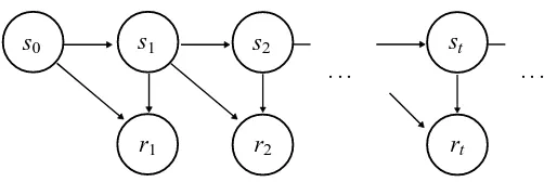
Figure 1: Graphical model for infinite horizon MRP. s and r denote state variable and reward, re-spectively.

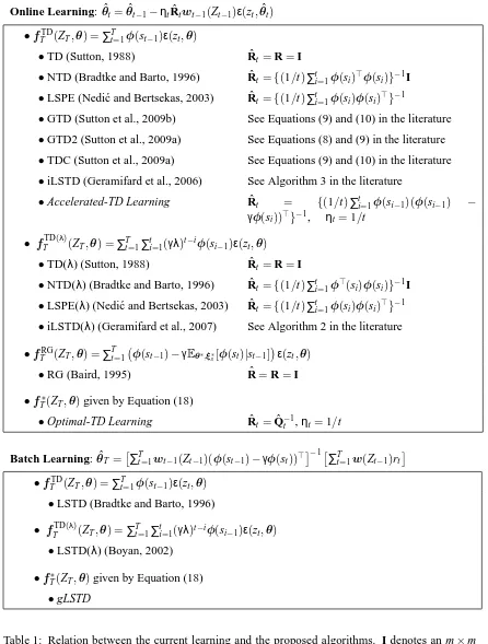
and Barto, 1998), Bellman residual (RG) learning (Baird, 1995), LSTD learning (Bradtke and Barto, 1996), LSTD(λ) learning (Boyan, 2002), least squares policy evaluation (LSPE) learning (Nedi´c and Bertsekas, 2003), and incremental LSTD (iLSTD) learning (Geramifard et al., 2006, 2007) (Table 1).

We compare the performance of the proposed online algorithms with a couple of well-established algorithms in simple numerical experiments and show that the results support our theoretical find-ings.

The rest of this article is organized as follows. First, we give background of MRP and define the semiparametric statistical model for estimating the value function (Section 2). After providing a short overview of estimating functions (Section 3), we present the main contribution, fundamen-tal statistical analysis based on the estimating function theory (Section 4). Then, we explain the construction of practical learning algorithms, derived from estimating functions, as both batch and online algorithms (Section 5). Furthermore, relations of our proposed methods to current algorithms in RL are discussed (Section 6). Finally, we report our experimental results (Section 7), and discuss open questions and future direction of this study (Section 8).

2. Markov Reward Processes

Figure 1 shows a graphical model for an infinite horizon MRP1which is defined by the initial state probability p(s0), the state transition probability p(st|st−1)and the reward probability p(rt|st,st−1). State variable s is an element of a finite set S and reward variable r_∈R can be either discrete or continuous. The joint distribution of a sample trajectory ZT ≡ {s0,s1,r1···,sT,rT}of the MRP is described as

p(ZT) =p(s0) T

∏

p(rt|st,st−1)p(st|st−1). (1)

We further impose the following assumptions on MRPs.

Assumption 1 Under p(st_|st₋1), the MRP has a unique invariant stationary distribution µ(s). Assumption 2 For any time t, reward rt is uniformly bounded.

Before introducing the statistical framework, we begin by confirming that the value function esti-mation can be interpreted as estiesti-mation of certain statistics of MRP (1).

Proposition 1 (Bertsekas and Tsitsiklis, 1996) Consider a conditional probability of_{rt,st}given st₋1,

p(rt,st_|st₋1) =p(rt|st,st−1)p(st|st−1). Then, there is such a function V that

E[rt|st−1] =V(st−1)−γE[V(st)|st−1] (2)

holds for any state st−1∈S, whereγ∈[0,1)is a constant called discount factor. Here,E[·|s]denotes the conditional expectation for the given state s. The function V that satisfies Equation (2) is unique and found to be the value function:

V(s)_≡ lim T_→∞E

" _T

∑

γt−1_rt

s0=s

#

. (3)

We assume throughout this article that the value function can be represented by a certain parametric function, even a nonlinear function with respect to its parameter.

Assumption 3 The value function given by Equation (3) is represented by a parametric function g(s,θ):

V(s) =g(s,θ).

Here, g : S_×Θ_7→R andθ_∈Θis a certain parameter in a parameter space Θ_⊆Rm. Also, the dimension of the parameterθis smaller than that of the state space: m<_|S_|. Moreover, g(s,θ)is assumed to be twice continuously differentiable with respect toθ.

Under Assumption 3, p(rt|st−1)is partially parametrized byθ, through its conditional mean

E[rt|st−1] =g(st−1,θ)−γE[g(st,θ)|st−1]. (4)

Our objective is to find out such a value of the parameter θ that function g(s,θ) satisfies Equa-tion (4), that is, it coincides with the true value funcEqua-tion.

To specify the probabilistic model (1) altogether, we usually need extra parameters other than θ. Let ξ0 and ξs be such additional parameters that p(s0,ξ0) and p(r,s|s;θ,ξs) can completely represent the initial and transition distributions, respectively. In such a case, the joint distribution of the trajectory ZT is expressed as

p(ZT;θ,ξ) =p(s0;ξ0) T

∏

p(rt,st|st−1;θ,ξs), (5)

whereξ_≡(ξ0,ξs).

may have innumerable degrees of freedom. Statistical models which contain such (possibly infinite-dimensional) nuisance parameters (ξ) in addition to the parameter of interest (θ), are called semi-parametric (Bickel et al., 1998; Amari and Kawanabe, 1997; van der Vaart, 2000). We emphasize that the nuisance parameters are necessary only for developing theoretical frameworks. In actual estimation procedures of the parameterθ, same as in other model-free policy evaluation algorithms, we neither define them concretely, nor estimate them. This can be achieved by using estimating functions which is a well-established technique to obtain a consistent estimator of the parameter without estimating the nuisance parameters (Godambe, 1960, 1991; Amari and Kawanabe, 1997; Huber and Ronchetti, 2009). The advantages of considering such semiparametric models behind the model-free policy evaluation are:

(a) we can characterize all possible model-free algorithms,

(b) we can discuss asymptotic properties of the estimators in a unified way and obtain the optimal one with the minimum estimation error.

We review the estimating function method in the next section.

3. Estimating Functions in Semiparametric Models

We begin with a short overview of the estimating function theory in the independent and identically distributed (i.i.d.) case and then discuss the MRP case in the next section. We consider a general semiparametric model p(x;θ,ξ), where θ is an m-dimensional parameter of interest and ξ is a nuisance parameter which can have infinite degrees of freedom. An m-dimensional vector function f ofxandθis called an estimating function (Godambe, 1960, 1991) when it satisfies the following conditions for anyθandξfor sufficiently large values of T ;

Eθ,ξ[f(x,θ)] =0, (6)

det_|A_{| 6}=0, where A=Eθ,ξ[∂θf(x,θ)], (7)

Eθ,ξkf(x,θ)k2<∞, (8)

where∂θ=∂/∂θis the partial derivative with respect toθ, and det| · |and|| · ||denote the

determi-nant and the Euclidean norm, respectively. HereEθ,ξ[·]means the expectation overxwith respect to the distribution p(x;θ,ξ)and we further remark that the parameterθinf(x,θ)andEθ,ξ[·]must

be the same.

Suppose i.i.d. samples _{x1,···,xT}are generated from the model p(x;θ∗,ξ∗). If there is an estimating functionf(x,θ), we can obtain an estimator ˆθT which has good asymptotic properties, by solving the following estimating equation:

T

∑

f(xt,θˆT) =0. (9)

A solution of the estimating Equation (9) is called an M-estimator in statistics (Huber and Ronchetti, 2009; van der Vaart, 2000). The M-estimator is consistent, that is, it converges to the true value regardless of the nuisance parameterξ∗.2 Moreover, it is normally distributed, that is,

0

θ∗ b

θ _θ

1

/

T∑

t

f

(

xt

,

θ

)

Figure 2: An illustrative plot of 1/T ∑t f(xt,θ)as function of θ(solid line). Due to the effect of finite samples, the function is slightly apart from its expectationEθ∗_,ξ∗[f(x,θ)](dashed line) which takes 0 atθ=θ∗because of condition (6). Condition (7) means that the expec-tation (dashed line) has a non-zero slope aroundθ∗, which ensures the local uniqueness of the zero crossing point. On the other hand, condition (8) guarantees that its standard deviation, shown by the two dotted lines, shrinks in the order of 1/√T , thus we can ex-pect to find asymptotically at least one solution ˆθT of estimating Equation (9) near the true valueθ∗. This situation holds regardless of the value of the true nuisance parameter

ξ∗_.

ˆ

θT ∼

N

Av_≡Av(θˆT) = 1 TA

−1

Eθ∗_,ξ∗

h

f(x,θ∗)f(x,θ∗)⊤i(A⊤)−1,

where A=Eθ∗_,ξ∗[∂_θf(x,θ∗)], and the symbol⊤denotes the matrix transpose. Note that the matrix Av depends on(θ∗,ξ∗), but not on the samples_{x1,···,xT}. We illustrate in Figure 2 the left side of the estimating Equation (9) normalized by the sample size T to explain why an M-estimator has good properties and to show the meaning of conditions (6)-(8).

4. Estimating Functions in MRP Model

The notion of estimating functions has been extended to be applicable to Markov time-series (Go-dambe, 1985, 1991; Wefelmeyer, 1996; Sørensen, 1999). We need a similar extension to enable it to be applied to MRPs. For convenience, we write the triplet at time t as zt ≡ {st−1,st,rt} ∈S2×R and the trajectory up to time t as Zt≡ {s0,s1,r1, . . . ,st,rt} ∈St+1×Rt.

Let us consider an m-dimensional vector-valued function of the formf_T: ST+1_×RT_×Θ_7→Rm:

fT(ZT,θ) = T

∑

This is similar to the left side of (9) in the i.i.d. case, but now each termψt : St+1×Rt×Θ7→Rm depends also on previous observations, that is, a function of the sequence up to time t. If the sequence of the functions_{ψt}satisfies the following properties for anyθ andξ, the functionfT becomes an estimating function for T sufficiently large (Godambe, 1985, 1991).

Eθ,ξs[ψt(Zt,θ)|Zt−1] =0, ∀t, (10)

det|A| 6=0, where A≡lim

t_→∞Eθ,ξ[∂θψt(Zt,θ)], (11)

lim t→∞Eθ,ξ

h

kψt(Zt,θ)k2

i

<∞. (12)

Note that the estimating functionfT(ZT,θ)satisfies the martingale properties because of condition (10). Therefore, it is called a martingale estimating function in the literature (Godambe, 1985, 1991; Wefelmeyer, 1996; Sørensen, 1999).3 Although time-series estimating functions can be defined in a more general form, the above definition is sufficient for our theoretical consideration.

4.1 Characterizing Class of Estimating Functions

In this section, we characterize possible estimating functions in MRPs. Let

ε: S2×R×Θ7→R1be the so-called temporal difference (TD) error, that is,

εt≡ε(zt,θ)≡g(st−1,θ)−γg(st,θ)−rt.

From Equation (4), its conditional expectationEθ,ξs[εt|Zt−1] =Eθ,ξs[εt|st−1]is equal to 0 for any t.

Furthermore, this zero-mean property holds even when multiplied by any weight function wt−1(Zt−1,θ), which depends on past observations and the parameter, that is,

Eθ,ξs[wt−1(Zt−1,θ)ε(zt,θ)|Zt−1] =wt−1(Zt−1,θ)Eθ,ξs[ε(zt,θ)|Zt−1] =0, (13)

for any t. We can obtain a class of possible estimating functions fT(ZT,θ) in MRPs from this observation if we impose some regularity conditions summarized in Assumption 4.

Assumption 4

(a) Functionwt : St+1×Rt×Θ7→Rm can be twice continuously differentiable with respect to parameterθfor any t, and lim

t→∞Eθ,ξ[|∂θwt(Zt,θ)|]<∞for anyθ.

(b) There exists a limit of matrixEθ,ξ[wt₋1(Zt₋1,θ){∂θε(zt,θ)}⊤], and the matrix

lim

t→∞Eθ,ξ[wt−1(Zt−1,θ){∂θε(zt,θ)}

⊤_{]is nonsingular for anyθandξ.}

(c) Eθ,ξ[kwt−1(Zt−1,θ)ε(zt,θ)k2]is finite for any t,θandξ.

3. Strictly speaking, strict consistency of M-estimator given by functionf(ZT,θ)requires some additional conditions.

Lemma 2 Suppose that random sequence ZT is generated from a distribution of semiparametric model_{p(ZT;θ,ξ)_|θ,ξ_}defined by Equation (5). If the conditions in Assumptions 1-4 are satisfied, then

fT(ZT,θ) = T

∑

ψt(Zt,θ)≡ T

∑

wt−1(Zt−1,θ)ε(zt,θ) (14) becomes an estimating function.

The proof is given in Appendix C. From Lemma 2, we can obtain an M-estimator ˆ

θT : ST+1×RT7→Rmby solving the estimating equation

T

∑

ψt(Zt,θˆT) =0. (15)

Practical procedures for finding the solution of the estimating Equation (15) will be discussed in Section 5. The estimator derived from the estimating Equation (15) has an asymptotic variance summarized in the following lemma.

Lemma 3 Suppose that random sequence ZT is generated from distribution p(ZT;θ∗,ξ∗). If the conditions in Assumptions 1-4 are satisfied, then the M-estimator derived from Equation (15) has asymptotic estimation variance

Av=Av(θˆT) = 1 TA

−1_ΣA⊤−1_{, (16)}

where A=A(θ∗,ξ∗) =lim t_→∞Eθ∗,ξ∗

h

wt−1(Zt−1,θ∗){∂θε(zt,θ∗)}⊤

i

,

Σ₌Σ_(θ∗_,ξ∗_{) =lim} t→∞Eθ∗,ξ∗

_ε

(zt,θ∗)2wt−1(Zt−1,θ∗)wt−1(Zt−1,θ∗)⊤

.

The proof is given in Appendix D. Interestingly, for the MRP model, we can specify all possi-ble estimating functions. More specifically, the converse of Lemma 2 also holds; any martingale estimating functions for MRP must take the form (14).

Theorem 4 Suppose that the conditions in Assumptions 1-4 are satisfied. Then, any martingale estimating functionfT(ZT,θ) =∑Tt=1ψt(Zt,θ)in the semiparametric model{p(ZT;θ,ξ)|θ,ξ}of MRP can be expressed as

fT(ZT,θ) = T

∑

ψt(Zt,θ) = T

∑

wt−1(Zt−1,θ)ε(zt,θ). (17) The proof is given in Appendix E.

4.2 Optimal Estimating Function

Lemma 5 Letwt(Zt,θ)be any weight function that depends on the current and previous observa-tions and the parameter, and satisfies the condiobserva-tions in Assumption 4. Then, there is necessarily a weight function depending only on the current state and the parameter whose corresponding esti-mator has the minimum asymptotic variance among all possible weight functions.

The proof is given in Appendix F.

We next discuss the optimal weight function of Equation (14) in terms of asymptotic variance, which corresponds to the optimal estimating function.

Theorem 6 Suppose that random sequence ZT is generated from distribution p(ZT;θ∗,ξ∗). If the conditions in Assumptions 1-4 are satisfied, an optimal estimating function with minimum asymp-totic estimation variance is given by

f_T∗(ZT,θ) =

T

∑

ψ∗_t(zt,θ)_≡

T

∑

w_t∗₋₁(st₋1,θ∗)ε(zt,θ), (18)

where

w_t∗₋₁(st−1,θ∗)≡Eθ∗_,ξ∗

s[ε(zt,θ

∗₎2

|st−1]−1Eθ∗_,ξ∗

s[∂θε(zt,θ

∗_)|s

t−1].

The proof is given in Appendix G. Note that weight functionw_t∗₋₁(Zt₋1,θ∗) depends on true pa-rameter θ∗ (unknown) and requires the expectation with respect to p(rt,st|st−1;θ∗,ξs∗), which is also unknown. Therefore, we need to approximate the true parameter and the expectation, which will be explained in a later section.

The asymptotic variance of the optimal estimating function can be calculated from Lemma 3 and Theorem 6.

Lemma 7 The minimum asymptotic variance is given by

Av=Av(θˆT) = 1 TQ

−1_,

where Q_≡lim

t→∞Eθ∗,ξ∗[∂θψ ∗

t(zt,θ∗)] =_tlim

→∞Eθ∗,ξ∗

ψ_t∗(zt,θ∗)ψ_t∗(zt,θ∗)⊤.

The proof is given in Appendix H. We here note that positive definite matrix Q is similar to the Fisher information matrix, which is well-known in asymptotic estimation theory. However, the in-formation associated with this matrix Q is generally smaller than the Fisher inin-formation because we sacrifice statistical efficiency for robustness against the nuisance parameter (Amari and Kawanabe, 1997; Amari and Cardoso, 2002). In other words, the estimator derived from the estimating function (18) does not achieve the statistical lower bound, that is, the Cram`er-Rao lower bound.4

5. Learning Algorithms

In this section, we present two kinds of practical algorithms to obtain the solution of the estimating Equation (15): one is the batch learning procedure and the other is the online learning procedure. In Section 5.1, we discuss batch learning and derive new least squares-type algorithms like LSTD and

LSTD(λ) to determine the parameterθ under the assumption that the value function is represented as a parametrically linear function. In Section 5.2, we then study convergence issues of online learning. We first analyze the sufficient condition of the convergence of the estimation and the convergence rate of various online procedures without the constraint of linear parametrization. This theoretical consideration allows us to obtain a new online learning algorithm that asymptotically converges faster than current online algorithms.

5.1 Batch Learning

Let g(s,θ)be a linear parametric function of features:

V(st)≡φ(st)⊤θ, (19)

whereφ: S_7→Rmis a feature vector andθ_∈Θis a parameter vector. Then, estimating Equation (14) is given as

T

∑

wt−1(Zt−1,θ)

n

(φ(st−1)−γφ(st))⊤θˆT−rt

o

=0_.

If the weight function does not depend on parameterθ, the estimator ˆθTcan be analytically obtained as

ˆ θT=

(

T

∑

¯

wt−1(Zt−1)(φ(st−1)−γφ(st))⊤

)−1( T

∑

¯

wt−1(Zt−1)rt

) ,

where ¯wt : St+1×Rt 7→Rmis a function which depends only on the previous observations. Note that when the weight function ¯w(Zt)is set toφ(st), this estimator is equivalent to that of the LSTD learning.

We now derive a new least-squares learning algorithm, generalized least squares temporal dif-ference (gLSTD), which achieves minimum estimation of asymptotic variance in linear estimations of value functions. If weight functionw_t∗(Zt,θ∗)defined in Theorem 6 is known, an estimator of the estimating function (18) can be obtained as

ˆ θT =

(

T

∑

w_t∗₋₁(Zt−1,θ∗)(φ(st−1)−γφ(st))⊤

)−1( T

∑

w_t∗₋₁(Zt−1,θ∗)rt

) ,

by recalling thatw_t∗₋₁(Zt₋1,θ∗) =Eθ∗_,ξ∗

s[ε(zt,θ∗)

2_|st

−1]−1Eθ∗_,ξ∗

s[φ(st−1)−γφ(st)|st−1]. Obviously,

we do not knoww_t∗₋₁(Zt−1,θ∗)because the definition ofwt∗−1(Zt−1,θ∗)contains the residual at the true parameter,ε(zt,θ∗), and unknown conditional expectations,Eθ∗_,ξ∗

s[ε(zt,θ∗)

2_|st

−1] andEθ∗_,ξ∗

s[φ(st−1)−γφ(st)|st−1]. Therefore, we replace the true residualε(zt,θ∗)with that of the

LSTD estimator and approximate the expectationsEθ∗_,ξ∗

s[ε(zt,θ

∗₎2_|s

t−1]−1and

Eθ∗_,ξ∗

s[φ(st−1)−γφ(st)|st−1]by using function approximations

Eθ∗_,ξ∗

s[ε(zt,θ

∗₎2

|st−1]−1≈v(st−1,α),

Eθ∗_,ξ∗

Algorithm 1 gLSTD learning for t=1,2,_··· do

Obtain sample zt={st−1,st,rt} end for

Set constant k to a sufficiently large value for t=1,2,_··· do

Calculate LSTD estimator ˆθLSTD_{based on sample}

{z1,_···,zt₋1} ∪ {zt+k,···,zT} Calculate its residual ˆεt

ˆ

εt←(φ(st₋1)−γφ(st))⊤θˆLSTD−rt

Calculate conditional expectations v(st−1,α),ζ(st−1,β)by means of function approximations based on sample{z1,_···,zt₋1} ∪ {zt+k,···,zT}

Obtain the weight function

ˆ

w_t∗_−1←v(st₋1,α)−1ζ(st−1,β) end for

Obtain the gLSTD estimator

ˆ

θ_TgLSTD_←[∑T_t=1wˆ_t∗₋₁(φ(st₋1)−γφ(st))⊤]−1[∑Tt=1wˆt∗₋1rt]

5.2 Online Learning

Online learning procedures in the field of RL are often preferred to batch learning ones because they require less memory and can be adapted even to time-variant situations. Here, an online estimator of θat time t is denoted as ˆθt. Suppose that sequence{ψ1(Z1,θ),···,ψT(ZT,θ)}forms a martingale estimating function for MRP. Then, an online update rule can simply be given by

ˆ

θt =θˆt−1−ηtψt(Zt,θˆt−1), (20) whereηt denotes a nonnegative scalar stepsize. In fact, there are other online update rules derived from the same estimating functionft(Zt,θ) =∑ti=1ψi(Zi,θ)as

ˆ

θt =θˆt−1−ηtR(θˆt−1)ψt(Zt,θˆt−1), (21) where R(θ)denotes an m_×m nonsingular matrix only depending onθ(Amari, 1998). This variation results from the fact that function R(θ)∑t

i=1ψi(Zi,θ)yields the same roots as its original for any R(θ). This equivalence guarantees that both learning procedures, (20) and (21), have the same equilibrium, while their dynamics may be different, that is, even if the original algorithm (20) is unstable around the required solution, it can be stabilized by introducing appropriate R(θ) into (21).

We will discuss the convergence of the online learning algorithm (21) in the next two subsec-tions.

5.2.1 CONVERGENCE TOTRUEVALUE

We will now discuss the convergence of online learning (21) to the true parameterθ∗. For the sake of simplicity, we will focus on local convergence, that is, initial estimator ˆθ0 is confined in the neighborhood of the true parameter, which is assumed to be a unique solution in the neighborhood. Now let us introduce sufficient conditions for convergence.

Assumption 5

(a) For any t,(θˆt−θ∗)⊤R(θˆt)Eθ∗_,ξ∗

s[ψt+1(Zt+1,θˆt)|st]is nonnegative. (b) For any t, there exists such nonnegative constants c1and c2that

Eθ∗_,ξ∗

s

h

R(θˆt)ψt+1(Zt+1,θˆt)

2sti_≤c1+c2θˆt−θ∗

2.

Condition (a) assumes that the opposite of gradient R(θˆt)Eθ∗_,ξ∗

s[ψt+1(Zt+1,θˆt)|st]must point toward

the true parameterθ∗at each time t. Then, the following theorem guarantees the convergence of ˆθt toθ∗.

Theorem 8 Suppose that random sequence ZT is generated from distribution p(ZT;θ∗,ξ∗). Also, suppose that the conditions in Assumptions 1-5 hold. If stepsizes _{ηt} are all positive and sat-isfy∑∞_t=1ηt =∞and∑t=1∞ η2t <∞, then the online algorithm (21) almost surely converges to true parameterθ∗.

5.2.2 CONVERGENCERATE

The convergence speed of an online algorithm could generally be slower than that of its batch counterpart that tries to solve the estimating equation using all available samples. However, if we set matrix R(θ)and stepsizes_{ηt}appropriately, then it is possible to achieve the same convergence speed as that of the batch algorithm (Amari, 1998; Murata and Amari, 1999; Bottou and LeCun, 2004, 2005). Following the discussion on the previous work (Bottou and LeCun, 2004, 2005), we elucidate the convergence speed of online learning for estimating the value function in this section. Throughout the following discussion, the notion of stochastic orders plays a central role. Appendix A briefly describes the definition of stochastic orders and their properties. Then, we characterize the learning process for the batch algorithm.

Lemma 9 Let ˜θt and ˜θt₋1be solutions to estimating equations

(1/t)∑t

i=1ψi(Zi,θ˜t) =0 and (1/(t−1))∑ti=1−1ψi(Zi,θ˜t−1) =0, respectively. We assume that the conditions in Assumptions 2-4 are satisfied. Also we assume that ˜θt is uniformly bounded for any t, and matrix ˜Rt(θ˜t₋1)≡(1/t)∑ti=1∂θψi(Zi,θ˜t₋1)is nonsingular for any t. Then, we have

˜

θt=θ˜t−1− 1 tR˜

−1

t (θ˜t−1)ψt(Zt,θ˜t−1) +Op

1 t2

, (22)

where the definition of Op(_·)is given in Appendix A.

The proof is given in Appendix J. Note that Equation (22) defines the sequence of ˜θt as a recursive stochastic process that is essentially the same as online learning (21) for the same R. In other words, Lemma 9 indicates that online algorithms can converge with the same convergence speed as their batch counterparts through an appropriate choice of matrix R. Finally, the following theorem addresses the convergence speed of the (stochastic) learning process such as that in Equation (22).

Theorem 10 Suppose that random sequence ZT is generated from distribution p(ZT;θ∗,ξ∗), and then consider the following learning process

ˆ

θt =θˆt−1− 1 tRˆ

−1

t ψt(Zt,θˆt−1) +Op

1 t2

, (23)

where ˆRt ≡ {(1/t)∑ti=1∂θψi(Zi,θˆi−1)}. Assume that: (a) For any t, ˆθt is uniformly bounded.

(b) ˆR_t−1can be written as ˆR_t−1=Eθ∗_,ξ∗

s[Rˆ

−1

t |Zt−1] +op(1/t). (c) Eθ∗_,ξ∗[∂_θψ_t(Zt,θ∗)θˆ_t−1θˆ⊤_t

−1]can be written as

Eθ∗_,ξ∗[∂θψt(Zt,θ∗)θˆt₋1θˆ⊤_t−1] =Eθ∗_,ξ∗[∂θψt(Zt,θ∗)]Eθ∗_,ξ∗[θˆt₋1θˆ⊤_t−1] +o(1/t). (d) For any t, ˆRtis a nonsingular matrix.

Also assume that the conditions in Assumptions 1-4 are satisfied. If learning process (23) almost surely converges to the true parameter, then the convergence rate is given as

Eθ∗_,ξ∗kθˆ_t−θ∗k2=1 ttr

n

A−1Σ_(A−1₎⊤

o

+o

1 t

where A=lim

t_→∞Eθ∗,ξ∗[wt−1(Zt−1,θ

∗_{){∂θε(zt,θ}∗_)}⊤_]and

Σ_=lim

t→∞Eθ∗,ξ∗[ε(zt,θ ∗₎2_w

t₋1(Zt₋1,θ∗)wt₋1(Zt₋1,θ∗)⊤].

The proof is given in Appendix K. Note that this convergence rate (24) is neither affected by the third term of (23) nor by the op(1/t)term in matrix ˆR−t 1.

5.2.3 GENERALIZEDTD LEARNING

We now present the online learning procedure that yields the minimum estimation error. Roughly speaking, this is given by estimating functionf_T∗(ZT,θ)in Theorem 6 with the best (i.e., with the fastest convergence) choice of the nonsingular matrix in Theorem 10:

ˆ

θt=θˆt−1− 1 tQˆ

−1

t ψ∗(zt,θˆt−1), (25) where ˆQt−1={(1/t)∑ti=1∂θψ∗(zi,θˆi−1)}−1 andψ∗(zt,θ)have been defined by Equation (18). If learning equation (25) satisfies conditions in Assumptions 1-5 and Theorem 10, then it converges to the true parameter with the minimum estimation error,(1/t)Q−1. However, this is impractical as learning rule (25) contains unknown parameters and quantities. For practical implementation, we need to evaluate Eθ∗_,ξ∗

s[ε(zt,θ∗)

2_|s

t−1] andEθ∗_,ξ∗

s[∂θε(zt,θ∗)|st−1]by using function

approxi-mations, whereas standard online learning procedures do not maintain statistics as a time series to avoid increasing the amount of memory. Therefore, we apply online functional approximations to these.

Let v(st,αt)andζ(st,βt)be the approximations ofEθ∗_,ξ∗

s[ε(zt+1,θt)

2_|st]and

Eθ∗_,ξ∗

s[∂θε(zt+1,θt)|st], respectively. Here, αt andβt are adjustable parameters, and they are

ad-justed in an online manner;

ˆ

αt=αˆt−1−ηαt ∂αv(st−1,αˆt−1){v(st−1,αˆt−1)−ε(zt,θˆt−1)2} ˆ

βt=βˆt−1−ηβt ∂βζ(st−1,βˆt−1){ζ(st−1,βˆt−1)−∂θε(zt,θˆt−1)},

whereη_tαandη_tβare stepsizes. By using these parametrized functions, we can replaceψ_t∗(zt,θˆt−1) and ˆQ−_t 1by

ψ∗_t(zt,θˆt−1) =v(st−1,αˆt−1)−1ζ(st−1,βˆt−1)ε(zt,θˆt−1) ˆ

Q−_t 1=

(

1 t

t

∑

v(si−1,αˆi−1)−1ζ(si−1,βˆi−1)∂θε(zi,θˆi−1)⊤

)₋1

. (26)

Note that update (26) can be done in an online manner by applying the well-known matrix inversion lemma (Horn and Johnson, 1985);

ˆ

Q−_t 1= 1 (1₋εt)

ˆ

Q_t−₋1₁₋ εt 1₋εt

ˆ

Q−_t−1₁wˆ_t∗₋₁∂θε(zt,θˆt−1)⊤Qˆ−t−11

(1₋εt) +εt∂θε(zt,θˆt₋1)⊤Qˆ_t−₋1₁wˆ_t∗₋₁

, (27)

whereεt≡1/t and ˆwt∗₋1≡v(st−1,αˆt−1)−1ζ(st−1,βˆt−1). Following Amari et al. (2000), we addi-tionally simplify update equation (27) as

ˆ

Algorithm 2 Optimal TD Learning

Initialize ˆα0, ˆβ0, ˆθ0, ˆQ−₀1=εIm, a1, a2

{εand Imdenote a small constant and an m×m identical matrix.} for t=1,2,_··· do

Obtain a new sample, zt={st−1,st,rt} Calculate the weight function, ˆw_t∗₋₁

ˆ

αt←αˆt₋1−ηαt ∂αv(st₋1,αˆt₋1){v(st₋1,αˆt₋1)−ε(zt,θˆt₋1)2} ˆ

β_t←βˆ_t−1−ηβ_t ∂βζ(st−1,βˆt−1){ζ(st−1,βˆt−1)−∂θε(zt,θˆt−1)} ˆ

w∗_t−1←v(st−1,αˆt−1)−1ζ(st−1,βˆt−1) Update ˆQ−_t 1by using Equation (28)

ˆ

Qt−1←(1+ (1/t))Qˆt−−11−(1/t)Qˆ− 1

t−1wˆt∗₋1∂θε(zt,θˆt−1)⊤Qˆ_t−₋1₁ Update the parameter,

τ←min(a1,a2/t) ˆ

θt ←θˆt−1−(1/τ)Qˆt−1wˆt∗₋1ε(zt,θˆt−1) end for

which can be obtained because εt is small. We call this procedure optimal TD learning and its pseudo-code is summarized in Algorithm 2.5

5.2.4 ACCELERATEDTD LEARNING

TD learning is a traditional online approach to model-free policy evaluation and has been one of the most important algorithms in the RL field. Although TD learning is widely used because of its simplicity, it is known that it converges rather slowly. This section discusses TD learning from the viewpoint of the method of estimating functions and proposes a new online algorithm that can achieve faster convergence than standard TD learning.

To simplify the following discussion, we have assumed that g(s,θ) is a linear function as in Equation (19) with which we can solve the linear estimating equation using both batch and online procedures. When weight functionwt(Zt,θ)in Equation (13) is set to φ(st), the online and batch procedures correspond to the TD and LSTD algorithms, respectively. Note that both TD and LSTD share the same estimating function. Therefore, from Lemma 9 and Theorem 10, we can theoretically construct accelerated TD learning, which converges at the same speed as LSTD learning.

Here, we consider the following learning equation:

ˆ

θt =θˆt−1− 1 tRˆ

−1

t φ(st−1)ε(zt,θˆt−1), (29) where ˆR−t 1={(1/t)∑ti=1φ(si−1)(φ(si₋1)−γφ(si))⊤}−1. Since ˆR−t 1converges to

A−1=lim

t→∞Eθ∗,ξ∗[φ(st−1)(φ(st−1)−γφ(st))

⊤_]−1 _{and A−}1 _{must be a positive definite matrix (see} Lemma 6.4 in Bertsekas and Tsitsiklis 1996), online algorithm (29) also almost surely converges to the true parameter. Then, if ˆRt satisfies the conditions in Theorem 10, it can achieve the same

Algorithm 3 Accelerated-TD Learning Initialize ˆθ0, ˆR−₀1=εIm, a1, a2

{εand Imdenote a small constant and an m×m identical matrix.} for t=1,2,_··· do

Obtain a new sample, zt={st−1,st,rt} Update ˆR−t 1

ˆ

R−_t 1_←(1+ (1/t))_Rˆ−1

t−1−(1/t)Rˆ− 1

t−1∂θg(st−1,θˆt−1)∂θε(zt,θˆt−1)Rˆ−t−11 Update the parameter,

τ_←min(a1,a2/t)

ˆ

θt ←θˆt−1−(1/τ)Rˆ−t 1∂θg(st−1,θˆt−1)ε(zt,θˆt−1) end for

convergence rate as LSTD. We call this procedure Accelerated-TD learning. We present an imple-mentation of Accelerated-TD learning in Algorithm 3.

6. Related Work

This section discusses the relation between current major RL algorithms and the proposed ones from the viewpoint of estimating functions. Theorem 4 describes the broadest class of estimating func-tions that lead to unbiased estimators. Therefore, almost all the current value-based RL methods, in which consistency is assured, can be viewed as instances of the method of estimating functions.

For simplicity, let g(s,θ)be a linear function, that is, the value function can be represented as in Equation (19). We have two ways of solving such a linear estimating equation. The first is a batch procedure:

ˆ θT=

"_T

∑

wt₋1(φ(st₋1)−γφ(st))⊤

#−1"_T

∑

wt₋1rt

# .

and the second is an online procedure:

ˆ

θt =θˆt₋1−ηtRtˆ wt₋1ε(zt,θˆt₋1),

wherewt is a weight function at time t. By choosing both weight functionwt₋1 and the learning procedure, we can derive various RL algorithms. LetfTD

T , f TD(λ)

T , fTRGandfT∗ be the estimating functions that are defined as

f_TTD_≡f_TTD(ZT,θ) = T

∑

φ(st−1)ε(zt,θ),

f_TTD(λ)_≡f_TTD(λ)(ZT,θ) =

T

∑

t

∑

(γλ)t−iφ(si₋1)ε(zt,θ),

f_TRG_≡f_TRG(ZT,θ) = T

∑

Eθ∗_,ξ∗

s[φ(st−1)−γφ(st)|st−1]ε(zt,θ),

f_T∗_≡f_T∗(ZT,θ) =

T

∑

Eθ∗_,ξ∗

s[(ε(zt,θ

∗₎2_|st

−1]−1Eθ∗_,ξ∗

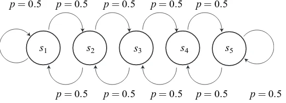
s1 s2 s3 s4 s5 p=0.5 p=0.5 p=0.5 p=0.5 p=0.5

p=0.5 p=0.5 p=0.5 p=0.5 p=0.5

Figure 3: A five-states MRP.

Here, we remark that TD-based algorithms (TD Sutton and Barto, 1998, NTD Bradtke and Barto, 1996, LSTD Bradtke and Barto, 1996, LSPE Nedi´c and Bertsekas, 2003, GTD Sutton et al., 2009b, GTD2, TDC Sutton et al., 2009a and iLSTD Geramifard et al., 2006), TD (λ)-based algorithms (TD (λ) Sutton and Barto, 1998, NTD (λ) Bradtke and Barto, 1996, LSTD (λ) Boyan, 2002, LSPE (λ) Nedi´c and Bertsekas, 2003, and iLSTD (λ) Geramifard et al., 2007) and RG (Baird, 1995) originated from the estimating functions fTD

T , f TD(λ)

T andfTRG, respectively. It should be noted that GTD, GTD2, GTDc, iLSTD, and iLSTD (λ) are specific online implementations for solving corresponding estimating equations; however, these algorithms can also be interpreted as instances of the method of estimating functions we propose. We have briefly summarized the relation between the current learning algorithms and the proposed algorithms in Table 1.

The asymptotic behavior of model-free policy evaluation has been analyzed within special con-texts; Konda (2002) derived the asymptotic variance of LSTD (λ) and revealed that the convergence rate of TD (λ) was worse than that of LSTD (λ). Yu and Bertsekas (2006) derived the convergence rate of LSPE (λ) and found that it had the same convergence rate as LSTD (λ). Because these results can be seen in Lemma 3 and Theorem 8, our proposed framework generalizes previous asymptotic analyses to provide us with a methodology that can be more widely applied to carry out asymptotic analyses.

7. Simulation Experiment

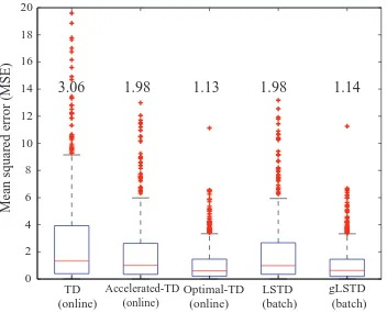
In order to validate our theoretical developments, we compared the performance (statistical error) of the proposed algorithms (gLSTD, Accelerated-TD and Optimal-TD algorithms) with those of the online and batch baselines: TD algorithm (Sutton and Barto, 1998) and LSTD algorithm (Bradtke and Barto, 1996), respectively, in a very simple problem. An MRP trajectory was generated from a simple Markov random walk on a chain with five states(s=1,_···,5)as depicted in Figure 3. At each time t, the state changes to either of its left (₋1) or right (+1) with equal probability of 0.5. A reward function was set as a deterministic function of the state:

r = [0.6594,₋0.3870,₋0.9742,₋0.9142,0.9714]6 _{and the discount factor was set to 0.95. The} value function was approximated by a linear function with three-dimensional basis functions, that is, V(s)_≈∑3

n=1θnφn(s). The basis functionsφn(s)were generated according to a diffusion model (Ma-hadevan and Maggioni, 2007); basis functions were given based on the minor eigenvectors of the

Online Learning: ˆθt =θˆt−1−ηtRtˆ wt−1(Zt−1)ε(zt,θˆt)

•fTD

T (ZT,θ) =∑Tt=1φ(st−1)ε(zt,θ)

•TD (Sutton, 1988) Rˆt =R=I

•NTD (Bradtke and Barto, 1996) Rtˆ =_{(1/t)∑_i=1t φ(si)⊤φ(si)_}−1_I

•LSPE (Nedi´c and Bertsekas, 2003) Rˆt ={(1/t)∑i=1t φ(si)φ(si)⊤}−1

•GTD (Sutton et al., 2009b) See Equations (9) and (10) in the literature

•GTD2 (Sutton et al., 2009a) See Equations (8) and (9) in the literature

•TDC (Sutton et al., 2009a) See Equations (9) and (10) in the literature

•iLSTD (Geramifard et al., 2006) See Algorithm 3 in the literature

•Accelerated-TD Learning Rˆt = {(1/t)∑ti=1φ(si−1)(φ(si−1) − γφ(si))⊤_}−1_, η

t=1/t

• f_TTD(λ)(ZT,θ) =∑_t=1T ∑t_i=1(γλ)t−i_φ(si

−1)ε(zt,θ)

•TD(λ) (Sutton, 1988) Rˆt =R=I

•NTD(λ) (Bradtke and Barto, 1996) Rtˆ =_{(1/t)∑t_i=1φ⊤(si)φ(si)_}−1_I

•LSPE(λ) (Nedi´c and Bertsekas, 2003) Rˆt ={(1/t)∑ti=1φ(si)φ(si)⊤}−1

•iLSTD(λ) (Geramifard et al., 2007) See Algorithm 2 in the literature

•fRG

T (ZT,θ) =∑t=1T φ(st−1)−γEθ∗_,ξ∗

s[φ(st)|st−1]

_ε

(zt,θ)

•RG (Baird, 1995) Rˆ =R=I

•f_T∗(ZT,θ)given by Equation (18)

•Optimal-TD Learning Rˆt =Qˆt−1,ηt=1/t

Batch Learning: ˆθT =

∑T

t=1wt−1(Zt−1)(φ(st−1)−γφ(st))⊤

−1 ∑T

t=1w(Zt−1)rt

•fTD

T (ZT,θ) =∑Tt=1φ(st−1)ε(zt,θ)

•LSTD (Bradtke and Barto, 1996)

• f_TTD(λ)(ZT,θ) =∑Tt=1∑ti=1(γλ)t−iφ(si−1)ε(zt,θ)

•LSTD(λ) (Boyan, 2002)

•f_T∗(ZT,θ)given by Equation (18)

•gLSTD

TD (online)

Accelerated-TD (online)

Optimal-TD (online)

LSTD (batch)

gLSTD (batch) 0

2 4 6 8 10 12 14 16 18 20

Mean squared error (MSE)

3.06

1.98

1.13

1.98

1.14

Figure 4: Boxplots of MSE both of the online (TD, Accelerated-TD and Optimal-TD) and batch (LSTD and gLSTD) algorithms. The center line, and the upper and lower sides of each box denote the median of MSE, and the upper and lower quartiles, respectively. The number above each box is the average MSE.

graph Laplacian on an undirected graph constructed by the state transition. The basis functions actu-ally used in this simulation wereφ(s1) = [1,−0.6015,0.5117]⊤,φ(s2) = [1,−0.3717,−0.1954]⊤, φ(s3) = [1,0,−0.6325]⊤,φ(s4) = [1,0.3717,−0.1954]⊤, andφ(s5) = [1,0.6015,0.5117]⊤. In gen-eral, there is no guarantee that the true value function is included in the space spanned by the gener-ated basis functions. In our example, however, the true value function can be represented faithfully by the basis vectors above.

We first generated M=500 trajectories (episodes) each of which consisted of T=500 random walk steps. The value function was estimated for each episode. We evaluated the mean squared error (MSE) between the true value function and the estimated value function, evaluated over the five states.

procedures. More specifically, the first 10 steps in each episode were used to obtain initial estimators in a batch manner and the online algorithm started after the 10 steps.

In the proposed online algorithms (Accelerated-TD and Optimal-TD), the stepsizes were de-creased as simple as 1/t. On the other hand, the convergence of TD learning was too slow in the sim-ple 1/t setting due to fast decay of the stepsizes; this slow convergence was also observed when em-ploying a certain well-chosen constant stepsize. Therefore, we adopt an ad-hoc adjustment for the stepsizes as 1/τ, whereτ=α0(n0+1)/(n0+t). The bestα0and n0have been selected by searching the sets ofα0∈ {0.05,0.1,0.2,0.3,0.4}and n0∈ {10,50,100,150,200,250,300,400,500,1000}, so thatα0and n0are selected as 0.3 and 200, respectively.

As shown in Figure 4, the Optimal-TD and gLSTD algorithms achieved the minimum MSE among the online and batch algorithms, respectively. The MSEs by these two methods were com-parable.7 It should be noted that the Accelerated-TD algorithm performed significantly better than the ordinary TD algorithm, showing the matrix R was effective for accelerating the convergence of the online procedure as expected by our theoretical analysis.

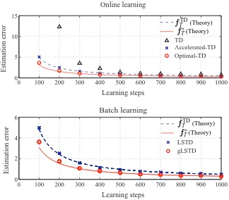
Figure 5 shows how the estimation error of the estimator ( ˆθT) behaves as the learning proceeds, both for online (upper panel) and batch (lower panel) learning algorithms. X-axis and y-axis denote the number of learning steps and the estimation error, that is, the MSE between the true parameter and estimated parameter, average over 500 runs, respectively. The theoretical results, dotted and solid lines, exhibit good accordance with the simulation results, crosses and circles, respectively, as expected. Although our theoretical methods were mostly based on asymptotic analysis, they were supported by simulation results even in the cases of relatively small number of samples.

8. Discussion and Future Work

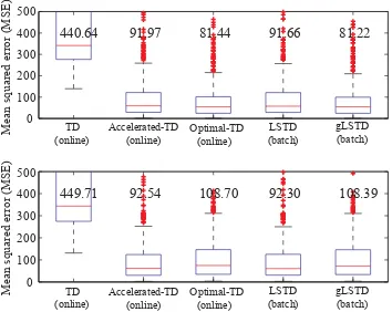
The contributions of this study are to present a new semiparametric approach to the model-free policy evaluation, which generalizes most of the current policy evaluation methods, and to clarify statistical properties of the policy evaluation problem. On the other hand, our framework to eval-uate the policy evaluation has been restricted to situations in which the function approximation is faithful, that is, there is no model misspecification for the value function; we have not referred to sta-tistical behaviors of our proposed algorithms in misspecified cases. In fact, the proposed algorithms may not better than current algorithms when the choice of parametric function g or the preparation of basis functions for approximating the value function introduces bias. Also, it is unsure whether our proposed online algorithms converge or not in misspecified cases. Figure 6 shows an example where the proposed algorithms (Optimal-TD and gLSTD) fail to obtain the best estimation accuracy. Here, an MRP trajectory was generated from an Markov random chain on the same dynamics as in Section 7. Rewards+1 and−1 were given when arriving at states ‘1’ and ‘20’, respectively, and the discounted factor was set at 0.98. Under this setting, we generated M=500 trajectories (episodes) each of which consisted of T =1000 random walk steps. We tested two linear function approxi-mations with eight-dimensional and four-dimensional basis functions, respectively, which were also generated by the diffusion model. The former basis functions cause a tiny bias which can be ignored, whereas the latter ones make a significant bias. The upper and lower panels in Figure 6 show the

0 100 200 300 400 500 600 700 800 900 1000 0

5 10 15

Learning steps

E

st

im

at

ion e

rror

Online learning

0 100 200 300 400 500 600 700 800 900 1000

0 2 4 6

Learning steps

E

st

im

at

ion e

rror

Batch learning

TD

Accelerated-TD Optimal-TD

LSTD gLSTD

f_TTD(Theory) fTD

T (Theory)

f_T∗(Theory) f_T∗(Theory)

Figure 5: 500 learning runs by varying the initial conditions were performed. (Upper panel) Trian-gles (_△), crosses (_×) and circles (_◦) denote the simulation results for TD, Accelerated-TD and Optimal-TD, respectively. They were averaged over the 500 runs. The dotted and solid lines show the theoretical results discussed in Lemma 3 for estimating functions fTD

T andfT∗described in Section 6. (Lower panel) Crosses (×) and circles (◦) denote the simulation results for LSTD and gLSTD, respectively.

TD (online)

Accelerated-TD (online)

Optimal-TD (online)

LSTD (batch)

gLSTD (batch)

0 100 200 300 400 500

M

ea

n s

qua

re

d e

rror (M

S

E

)

440.64

91.97

81.44

91.66

81.22

0 100 200 300 400 500

M

ea

n s

qua

re

d e

rror (M

S

E

)

449.71

92.54

108.70

92.30

108.39

TD (online)

Accelerated-TD (online)

Optimal-TD (online)

LSTD (batch)

gLSTD (batch)

Figure 6: Boxplots of MSE for both of the online (TD, Accelerated-TD and Optimal-TD) and batch (LSTD and gLSTD) algorithms on a twenty states Markov random walk problem. (Upper panel) Simulation results on the function approximation with eight-dimensional diffusion basis functions. (Lower panel) Simulation results on the function approximation with four-dimensional diffusion basis functions.

8.1 Asymptotic Analysis in Misspecified Situations

First, let us revisit the asymptotic variance of the estimating function (15). In misspecified cases, estimating function (14) does not necessarily satisfy the martingale property, then its asymptotic variance can no longer be calculated by Equation (16). However, by introducing a notion of uniform mixing, the asymptotic variance can be correctly evaluated, even in misspecified cases.

To clarify the following discussion, we only consider the class of estimators given by the fol-lowing estimating function ¯fT : ST+1×RT×Θ7→Rm:

¯

fT(ZT,θ) = T

∑

¯

ψt(Zt,θ)≡ T

∑

¯

wt−1(Zt−1)ε(zt,θ). (30)

with Lemma 11 that the asymptotic variance of the estimators ˆθT given by the estimating equation

T

∑

¯

ψt(Zt,θˆ) =0. (31)

Lemma 11 Suppose that the random sequence ZT is generated from the distribution p(ZT)defined by Equation (1). Assume that:

(a) There exists such a parameter value ¯θ_∈Θthat

lim t→∞E

_¯

ψt(Zt,θ¯)

=0_,

where thatE[_·]denotes the expectation with respect to p(ZT), and ˆθT converges to the pa-rameter ¯θin probability.8

(b) There exists a limit of matrix Ew¯t−1(Zt−1){∂θε(zt,θ¯)}⊤

and lim

t→∞E

¯

wt−1(Zt−1){∂θε(zt,θ¯)}⊤

is nonsingular.

(c) Ekw¯_t−1(Zt−1)ε(zt,θ¯)k2

is finite for any t.

Then, the estimator derived from estimating Equation (31) has the asymptotic variance

f

Av_≡Avf(θˆT)≡E

h

(θˆT−θ¯)(θˆT−θ¯)⊤

i

= 1

TA¯

−1_{Σ¯ A¯}⊤−1_{, (32)}

where

¯

A_≡A¯(θ¯)_≡lim t→∞E

h

¯ wt−1

_∂

θε(zt,θ¯) ⊤

i ,

¯

Σ_≡Σ¯_(θ¯_)≡lim t_→∞E

h

ε(zt,θ¯)2w¯t−1w¯t⊤−1

i

+lim

t_→∞2 ∞

∑

covε(zt,θ¯)w¯t−1,ε(zt+t′,θ¯)w¯_t+t′₋₁.

Here, ¯wt and cov[·,·]denote the abbreviation of ¯wt(Zt)and the covariance function, respectively. The proof is given in Appendix L. Since this proof required the central limit theorem under uni-form mixing condition, we briefly review the notion and properties of uniuni-form mixing in Appendix B. We note that the infinite sum of covariance in Equation (32) becomes zero when the parametric representation of the value function is faithful. This implies that Lemma 11 generalizes the result of Lemma 3.

Furthermore, we can derive the upper bound of the asymptotic variance (32).

Lemma 12 There exists such a positive constantϒthat

1 TA¯

−1_{Σ¯ A¯}⊤−1 ϒ

TA¯

−1_Σ¯ 0

¯ A⊤

₋1

holds, where ¯Σ_0≡lim t→∞E

_ε

(zt,θ¯)2_w¯

t−1w¯_t⊤₋₁

.

8. We can show the stochastic convergence of the estimator to the parameter ¯θby imposing further mild conditions to ¯

The proof is given in Appendix M. This lemma addresses that the estimators, which we have proposed so far, minimize the upper bound of the asymptotic variance in misspecified cases.

Lemma 11 allows us to see the asymptotic behavior of the risk, like done by the previous work in a different context; Liang and Jordan (2008) evaluated the quality of probabilistic model-based pre-dictions in a structured prediction task. They analyzed the expected log-loss (risk) of composite like-lihood estimators and compared it with those of generative, discriminative and pseudo-likelike-lihood estimators, both when the probabilistic models are well-specified and misspecified. Since composite likelihood estimators are in the class of M-estimator, we will be able to evaluate the risk of vari-ous estimators by performing a similar analysis to Liang and Jordan (2008). Konishi and Kitagawa (1996) introduced generalized information criterion (GIC) which could be applied to evaluate statis-tical models constructed by various types of estimation procedures. GIC is the generalization of the well-known Akaike information criterion (AIC) (Akaike, 1974) and provided an unbiased estimator for the expected log-loss (risk) of statistical models obtained by M-estimators. Therefore, it may be possible to select a good model from a set of potential models by constructing an information criterion for model-free policy evaluation based on the analysis in Konishi and Kitagawa (1996).

8.2 Online Learning Procedures in Large Scale Situations

In both Optimal-TD and Accelerated-TD learning, it is necessary to maintain the inverse of the scaling matrix ˆRt. Since this matrix inversion operation costs O(m2)in each step, maintaining the inverse matrix becomes expensive when the dimensionality of the parameters increases. An effi-cient implementation in such a large-scale setting is to use a coarsely-represented scale matrix, for example, a diagonal or a block diagonal matrix. An appropriate setting still ensures the conver-gence rate of O(1/t)without losing the computational efficiency. Le Roux et al. (2008) presented an interesting implementation of natural gradient learning (Amari, 1998) for large-scale settings, which was called “TONGA”. TONGA uses a low-rank approximation of the scaling matrix and casted both problems of finding the low-rank approximation and computing the gradient onto a lower-dimensional space, thereby attaining a lower computational complexity. Therefore, by apply-ing such an idea to our proposed algorithms, we can improve the computational complexity without sacrificing the fast convergence.

9. Conclusions

Acknowledgments

This study was partly supported by Grant-in-Aid for Scientific Research (B) (No.21300113) from Japan Society for the Promotion of Science (JSPS) and the Federal Ministry of Economics and Technology of Germany (BMWi) under the project THESEUS, grant 01MQ07018. Tsuyoshi Ueno was also supported by JSPS Fellowship for Young Scientist.

Appendix A. Stochastic Order Symbols

The stochastic order symbols Op and op are useful when evaluating the rate of convergence by means of asymptotic theory. Let n denote the number of observations. The stochastic order symbols are defined as follows.

Definition 13 Let_{Xn} and{Rn}denote a sequence of random variables and a sequence of real numbers, respectively. Then Xn=op(Rn) if and only if Xn/Rnconverges in probability to 0 when n_→∞.

Definition 14 Let_{Xn} and{Rn}denote a sequence of random variables and a sequence of real numbers, respectively. Then Xn =Op(Rn) if and only if Xn/Rn is bounded in probability when n_→∞. “Bounded in probability” means that there exist a constant C_ε and a natural number n0(ε)

such that for anyε>0 and n>n0(ε),

P_{|Xn| ≤Cε} ≥1−ε

holds.

Most properties of the usual orders also apply to stochastic orders. For instance,

op(1) +op(1) =op(1),

op(1) +Op(1) =Op(1),

Op(1)op(1) =op(1),

(1+op(1))−1=Op(1),

op(Rn) =Rnop(1),

Op(Rn) =RnOp(1),

op(Op(1)) =op(1).

Moreover, by taking the expectation, the stochastic order symbol op(·) reduces to the usual order symbol o(_·).

Remark 15 Let_{Xn_}and_{Rn_}denote a sequence of random variables which satisfies Xn=op(1)

and a sequence of real numbers, respectively. Let Yn =XnRn denote a random variable which satisfies Yn=op(Rn). If the sequence of random variable Ynis asymptotically uniformly integrable, then, the expectation of the random variables Ynhas the same normal order,E[Yn] =o(Rn).