Learning from Examples as an Inverse Problem

Learning from Examples as an Inverse Problem

Ernesto De Vito [email protected]

Dipartimento di Matematica

Universit`a di Modena e Reggio Emilia Modena, Italy

and INFN, Sezione di Genova,

Genova, Italy

Lorenzo Rosasco [email protected]

Andrea Caponnetto [email protected]

Umberto De Giovannini [email protected]

Francesca Odone [email protected]

DISI

Universit`a di Genova,

Genova, Italy

Editor: Peter Bartlett

Abstract

Many works related learning from examples to regularization techniques for inverse problems,

em-phasizing the strong algorithmic and conceptual analogy of certain learning algorithms with regu-larization algorithms. In particular it is well known that reguregu-larization schemes such as Tikhonov

regularization can be effectively used in the context of learning and are closely related to

algo-rithms such as support vector machines. Nevertheless the connection with inverse problem was considered only for the discrete (finite sample) problem and the probabilistic aspects of learning

from examples were not taken into account. In this paper we provide a natural extension of such

analysis to the continuous (population) case and study the interplay between the discrete and con-tinuous problems. From a theoretical point of view, this allows to draw a clear connection between

the consistency approach in learning theory and the stability convergence property in ill-posed

in-verse problems. The main mathematical result of the paper is a new probabilistic bound for the

regularized least-squares algorithm. By means of standard results on the approximation term, the consistency of the algorithm easily follows.

1. Introduction

The main goal of learning from examples is to infer an estimator from a finite set of examples. The

crucial aspect in the problem is that the examples are drawn according to a fixed but unknown prob-abilistic input-output relation and the desired property of the selected function is to be descriptive

also of new data, i.e. it should generalize. The fundamental work of Vapnik and further develop-ments (see Vapnik (1998); Alon et al. (1997) and Bartlett and Mendelson (2002) for recent results)

show that the key to obtain a meaningful solution is to control the complexity of the hypothesis

space. Interestingly, as pointed out in a number of papers (see Poggio and Girosi (1992); Evgeniou et al. (2000) and references therein), this is in essence the idea underlying regularization techniques

for ill-posed problems (Tikhonov and Arsenin, 1977; Engl et al., 1996). Not surprisingly the form of the algorithms proposed in both theories is strikingly similar (Mukherjee et al., 2002) and the point

of view of regularization is indeed not new to learning (Poggio and Girosi, 1992; Evgeniou et al., 2000; Vapnik, 1998; Arbib, 1995; Fine, 1999; Kecman, 2001; Sch¨olkopf and Smola, 2002). In

par-ticular it allowed to cast a large class of algorithms in a common framework, namely regularization

networks or regularized kernel methods (Evgeniou et al., 2000; Sch¨olkopf and Smola, 2002). Anyway a careful analysis shows that a rigorous mathematical connection between learning

the-ory and the thethe-ory of ill-posed inverse problems is not straightforward since the settings underlying the two theories are different. In fact learning theory is intrinsically probabilistic whereas the theory

of inverse problem is mostly deterministic. Statistical methods were recently applied in the context

of inverse problems (Kaipio and Somersalo, 2005). Anyway a Bayesian point of view is considered which differs from the usual learning theory approach. Recently the connection between learning

and inverse problems was considered in the restricted setting in which the elements of the input space are fixed and not probabilistically drawn (Mukherjee et al., 2004; Kurkova, 2004). This

cor-responds to what is usually called nonparametric regression with fixed design (Gy¨orfi et al., 1996)

and when the noise level is fixed and known, the problem is well studied in the context of inverse problems (Bertero et al., 1988). In the case of fixed design on a finite grid the problem is mostly that

we are dealing with an ill-conditioned problem, that is unstable w.r.t. the data. Though such setting is indeed close to the algorithmic setting from a theoretical perspective it is not general enough to

allow a consistency analysis of a given algorithm since it does not take care of the random sampling

providing the data. In this paper we extend the analysis to the setting of nonparametric regression with random design (Gy¨orfi et al., 1996).

Our analysis and contribution develop in two steps. First, we study the mathematical con-nections between learning theory and inverse problems theory. We consider the specific case of

quadratic loss and analyse the population case (i.e. when the probability distribution is known) to show that the discrete inverse problem which is solved in practice can be seen as the stochastic

discretization of an infinite dimensional inverse problem. This ideal problem is, in general,ill-posed

fi-nal goal in learning theory. This clarifies in particular the following important fact. Regularized solutions in learning problems should not only provide stable approximate solutions to the discrete

problem but especially give continuous estimates of the solution to the ill-posed infinite dimensional problem. Second, we exploit the established connection to study the regularized least-squares

al-gorithm. This passes through the definition of a natural notion of discretization noise providing a

straightforward relation between the number of available data and the noise affecting the problem. Classical regularization theory results can be easily adapted to the needs of learning. In

partic-ular our definition of noise together with well-known results concerning Tikhonov regpartic-ularization for inverse problems with modelling error can be applied to derive a new probabilistic bound for

the estimation error of regularized least squares improving recently proposed results (Cucker and Smale, 2002a; De Vito et al., 2004). The approximation term can be studied through classical

spec-tral theory arguments. The consistency of the algorithm easily follows. As the major aim of the

paper was to investigate the relation between learning from examples and inverse problem we just prove convergence without dealing with rates. Anyway the approach proposed in Cucker and Smale

(2002a); De Vito et al. (2004) to study the approximation term can be straightforwardly applied to derive explicit rates under suitable a priori conditions.

Several theoretical results are available on regularized kernel methods for large class of loss

functions. The stability approach proposed in Bousquet and Elisseeff (2002) allows to find data-dependent generalization bounds. In Steinwart (2004) it is proved that such results as well as other

probabilistic bounds can be used to derive consistency results without convergence rates. For the specific case of regularized least-squares algorithm a functional analytical approach to derive

consis-tency results for regularized least squares was proposed in Cucker and Smale (2002a) and eventually

refined in De Vito et al. (2004) and Smale and Zhou (2004b). In the latter the connection between learning and sampling theory is investigated. Some weaker results in the same spirit of those

pre-sented in this paper can be found in Rudin (2004). Anyway none of the mentioned papers exploit the connection with inverse problems. The arguments used to derive our results are close to those used

in the study of stochastic inverse problems discussed in Vapnik (1998). From the algorithmic point

of view Ong and Canu (2004) apply other techniques than Tikhonov regularization in the context of learning. In particular several iterative algorithms are considered and convergence with respect to

the regularization parameter (semiconvergence) is proved.

The paper is organized as follows. After recalling the main concepts and notation of statistical

learning (Section 2) and of inverse problems (Section 3), in Section 4 we develop a formal connec-tion between the two theories. In Secconnec-tion 5 the main results are stated, discussed and proved. In the

Appendix we collect some technical results we need in our proofs. Finally in Section 6 we conclude

2. Learning from Examples

We briefly recall some basic concepts of statistical learning theory (for details see Vapnik (1998);

Evgeniou et al. (2000); Sch¨olkopf and Smola (2002); Cucker and Smale (2002b) and references therein).

In the framework of learning from examples, there are two sets of variables: the input space X , which we assume to be a compact subset ofRn_{, and the output space Y , which is a subset of}R

contained in[₋M,M]for some M_≥0. The relation between the input x_∈X and the output y_∈Y is

described by a probability distributionρ(x,y) =ν(x)ρ(y|x)on X×Y . The distributionρis known only through a sample z= (x,y) = ((x1,y1), . . . ,(x`,y`)), called training set, drawn independently

and identically distributed (i.i.d.) according toρ. Given the sample z, the aim of learning theory is to find a function fz: X→Rsuch that fz(x)is a good estimate of the output y when a new input x is

given. The function fzis called estimator and the map providing fz, for any training set z, is called

learning algorithm.

Given a measurable function f : X_→R_{, the ability of f to describe the distribution}ρ_{is measured}

by its expected risk defined as

I[f] = Z

X×Y

V(f(x),y)dρ(x,y),

where V(f(x),y)is the loss function, which measures the cost paid by replacing the true label y with

the estimate f(x). In this paper we consider the square loss

V(f(x),y) = (f(x)₋y)2.

With this choice, it is well known that the regression function

g(x) = Z

Y

y dρ(y_|x)

is well defined (since Y is bounded) and is the minimizer of the expected risk over the space of all the measurable real functions on X . In this sense g can be seen as the ideal estimator of the

distribution probabilityρ. However, the regression function cannot be reconstructed exactly since only a finite, possibly small, set of examples z is given.

To overcome this problem, in the framework of the regularized least squares algorithm (Wahba,

1990; Poggio and Girosi, 1992; Cucker and Smale, 2002b; Zhang, 2003), an hypothesis space

H

of functions is fixed and the estimator fzλis defined as the solution of the regularized least squares

problem,

min f∈H{

1

` `

∑

i=1

(f(xi)−yi)2+λΩ(f)}, (1) where Ωis a penalty term andλ is a positive parameter to be chosen in order to ensure that the discrepancy.

I[fzλ]− inf

is small with high probability. Sinceρis unknown, the above difference is studied by means of a probabilistic bound

B

(λ, `,η), which is a function depending on the regularization parameterλ, the

number`of examples and the confidence level 1₋η, such that

P

I[fzλ]− inf f∈HI[f]≤

B

(λ, `,η)

≥1₋η.

We notice that, in general, inff_∈HI[f]is larger than I[g]and represents a sort of irreducible error

(Hastie et al., 2001) associated with the choice of the space

H

. We do not require the infimum

inf_f∈HI[f]to be achieved. If the minimum on

H

exists, we denote the minimizer by fH.

In particular, the learning algorithm is consistent if it is possible to choose the regularization

parameter, as a function of the available dataλ=λ(`,z), in such a way that

lim

`→+∞P

I[fzλ(`,z)]− inf

f∈HI[f]≥ε

=0, (2)

for everyε>0. The above convergence in probability is usually called (weak) consistency of the

algorithm (see Devroye et al. (1996) for a discussion on the different kind of consistencies). In this paper we assume that the hypothesis space

H

is a reproducing kernel Hilbert space

(RKHS) on X with a continuous kernel K. We recall the following facts (Aronszajn, 1950; Schwartz,

1964). The kernel K : X_×X _→R _{is a continuous symmetric positive definite function, where}

positive definite means that

∑

i,j

aiajK(xi,xj)≥0.

for any x1, . . .xn∈X and a1, . . .an∈R.

The space

H

is a real separable Hilbert space whose elements are real continuous functions

defined on X . In particular, the functions Kx=K(·,x)belong to

H

for all x∈X , and

H

= span_{Kx|x∈X}

hKx,KtiH = K(x,t) ∀x,t∈X,

where_h·,_·iH is the scalar product in

H

. Moreover, since the kernel is continuous and X is compact

κ=sup x∈X

p

K(x,x) =sup x∈Xk

KxkH <+∞, (3)

where_k·kH is the norm in

H

. Finally, given x_∈X , the following reproducing property holds

f(x) =_hf,KxiH ∀f ∈

H

. (4)

In particular, in the learning algorithm (1) we choose the penalty term

Ω(f) =_kf_kH2,

so that, by a standard convex analysis argument, the minimizer fzλ exists, is unique and can be

computed by solving a linear finite dimensional problem, (Wahba, 1990).

3. Ill-Posed Inverse Problems and Regularization

In this section we give a very brief account of the main concepts of linear inverse problems and

regularization theory (see Tikhonov and Arsenin (1977); Groetsch (1984); Bertero et al. (1985, 1988); Engl et al. (1996); Tikhonov et al. (1995) and references therein).

Let

H

and

K

be two Hilbert spaces and A :

H

_→

K

a linear bounded operator. Consider the equation

A f =g (5)

where g_∈

K

is the exact datum. Finding the function f satisfying the above equation, given A and

g, is the linear inverse problem associated to (5). In general the above problem is ill-posed, that is, the solution either not exists, is not unique or does not depend continuously on the datum g.

Existence and uniqueness can be restored introducing the Moore-Penrose generalized solution f† defined as the minimal norm solution of the least squares problem

min

f∈HkA f−gk

2

K. (6)

It can be shown (Tikhonov et al., 1995) that the generalized solution f† exists if and only if Pg∈

Range(A), where P is the projection on the closure of the range of A. However, the generalized

solution f† does not depend continuously on the datum g, so that finding f† is again an ill-posed problem. This is a problem since the exact datum g is not known, but only a noisy datum g_δ∈

K

is

given, where_kg₋g_{δkK ≤}δ. According to Tikhonov regularization (Tikhonov and Arsenin, 1977) a possible way to find a solution depending continuously on the data is to replace Problem (6) with

the following convex problem

min

f∈H{kA f−gδk

2

K+λkfk2H}, (7)

and, forλ>0, the unique minimizer is given by

f_δλ= (A∗A+λI)−1A∗g_δ, (8) where A∗the adjoint operator of A. A crucial issue is the choice of the regularization parameterλ

as a function of the noise. A basic requirement is that the reconstruction error

f

λ δ −f†

_H

is small. In particular,λmust be selected, as a function of the noise levelδand the data g_δ, in such

a way that the regularized solution f_δλ(δ,gδ)converges to the generalized solution, that is,

lim

δ→0 f

λ(δ,g_δ)

δ −f†

_H =0, (9)

Remark 1 We briefly comment on the well known difference between ill-posed and ill-conditioned

problems (Bertero et al., 1988). Finite dimensional problems are often well-posed. In particular it

can be shown that if a solution exists unique then continuity of A−1 is always ensured. Nonethe-less regularization is needed since the problems are usually ill conditioned and lead to unstable

solutions.

Sometimes, another measure of the error, namely the residual, is considered according to the

fol-lowing definition

A f

λ

δ −Pg

_K =

A f

λ δ −A f†

_K, (10) which will be important in our analysis of learning. Comparing (9) and (10), it is clear that while

studying the convergence of the residual we do not have to assume that the generalized solution exists.

We conclude this section noting that the above formalism can be easily extended to the case of a noisy operator A_δ:

H

_→

K

where

kA₋A_{δk ≤}δ,

and_k·kis the operator norm (Tikhonov et al., 1995).

4. Learning as an Inverse Problem

The similarity between regularized least squares and Tikhonov regularization is apparent comparing Problems (1) and (7). However while trying to formalize this analogy several difficulties emerge.

• To treat the problem of learning in the setting of ill-posed inverse problems we have to define a direct problem by means of a suitable operator A between two Hilbert spaces

H

and

K

.

• The nature of the noiseδin the context of statistical learning is not clear .

• We have to clarify the relation between consistency, expressed by (2), and the convergence considered in (9).

In the following we present a possible way to tackle these problems and show the problem of learn-ing can be indeed rephrased in a framework close to the one presented in the previous section.

We let L2(X,ν) be the Hilbert space of square integrable functions on X with respect to the marginal measureνand we define the operator A :

H

_→L2(X,ν)as

(A f)(x) =_hf,KxiH,

where K is the reproducing kernel of

H

. The fact that K is bounded, see (3), ensures that A is a

an element f is simply

(A f)(x) =f(x) _∀x_∈x, f _∈

H

,

that is, A is the canonical inclusion of

H

into L2_(X,ν_{). However it is important to note that A} changes the norm since_kf_kH is different to_kf_kL2_(X,ν). Second, to avoid pathologies connected with subsets of zero measure, we assume thatνis not degenerate.1 This condition and the fact that K is continuous ensure that A is injective (see the Appendix for the proof).

It is known that, considering the quadratic loss function, the expected risk can be written as

I[f] = Z

X

(f(x)₋g(x))2dν(x) + Z

X×Y

(y₋g(x))2dρ(x,y) = _kf₋g_k2_L2_(X,ν₎+I[g],

where g is the regression function (Cucker and Smale, 2002b) and f is any function in L2(X,ν). If f belongs to the hypothesis space

H

, the definition of the operator A allows to write

I[f] =_kA f₋g_k2_L2_(X,ν)+I[g]. (11) Moreover, if P is the projection on the closure of the range of A, that is, the closure of

H

into

L2(X,ν), then the definition of projection gives inf

f∈HkA f−gk

2

L2_(X,ν₎=kg−Pgk2_L2_(X,ν₎. (12) Given f _∈

H

, clearly PA f =A f , so that

I[f]₋ inf

f∈HI[f] =kA f−gk

2

L2_(X,ν)− kg−Pgk2_L2_(X,ν)=kA f−Pgk2_L2_(X,ν), (13) which is the square of the residual of f .

Now, comparing (11) and (6), it is clear that the expected risk admits a minimizer fH on the

hypothesis space

H

if and only if fH is precisely the generalized solution f†of the linear inverse

problem

A f =g. (14)

The fact that fH is the minimal norm solution of the least squares problem is ensured by the fact

that A is injective.

Let now z= (x,y) = ((x1,y1), . . . ,(x`,y`))be the training set. The above arguments can be repeated replacing the set X with the finite set_{x1, . . . ,x`}. We now get a discretized version of A

by defining the sampling operator (Smale and Zhou, 2004a)

Ax:

H

→E` (Axf)i=hf,KxiiH = f(xi),

where E`=R`_{is the finite dimensional euclidean space endowed with the scalar product}

w,w0

E`=

1

` `

∑

i=1 wiw0i.

It is straightforward to check that

1

` `

∑

i=1

(f(xi)−yi)2=kAxf−yk2E`,

so that the estimator fzλ given by the regularized least squares algorithm, see Problem (1), is the

Tikhonov regularized solution of the discrete problem

Axf=y. (15)

At this point it is useful to remark the following three facts. First, in learning from examples rather

than finding a stable approximation to the solution of the noisy (discrete) Problem (15), we want to find a meaningful approximation to the solution of the exact (continuous) Problem (14) (compare

with Kurkova (2004)). Second, in statistical learning theory, the key quantity is the residual of the

solution, which is a weaker measure than the reconstruction error, usually studied in the inverse problem setting. In particular, consistency requires a weaker kind of convergence than the one

usually studied in the context of inverse problems . Third, we observe that in the context of learning the existence of the minimizer fH, that is, of the generalized solution, is no longer needed to define

good asymptotic behavior. In fact when the projection of the regression function is not in the range

of A the ideal solution fH does not exist but this is not a problem since Eq. (12) still holds.

After this preliminary considerations in the next section we further develop our analysis stating

the main mathematical results of this paper.

5. Regularization, Stochastic Noise and Consistency

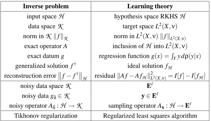
Table 1 compares the classical framework of inverse problems (see Section 3) with the formulation

of learning proposed above. We note some differences. First, the noisy data space E` is different

from the exact data space L2(X,ν) so that A and Ax belong to different spaces, as well as g and y. A measure of the difference between Ax and A, and between g and y is then required. Second,

both Axand y are random variables and we need to relate the noiseδto the number`of examples

in the training set z. Given the above premise our derivation of consistency results is developed

in two steps: we first study the residual of the solution by means of a measure of the noise due to

Inverse problem Learning theory

input space

H

hypothesis space RKHS

H

data space

K

target space L2(X,ν)

norm in

K

_kf_kK norm in L2(X,ν)_kf_kL2_(X,ν₎ exact operator A inclusion of

H

into L2(X,ν)

exact datum g regression function g(x) =R

Yy dρ(y|x) generalized solution f† ideal solution fH

reconstruction errorf−f†

_H residualkA f−A f_Hk2_L2_(X,ν)=I[f]−I[f_H]

noisy data space

K

E`

noisy data g_δ∈

K

y_∈E`

noisy operator A_δ:

H

_→

K

sampling operator Ax:

H

→E`

Tikhonov regularization Regularized least squares algorithm

Table 1: The above table summarizes the relation between the theory of inverse problem and the

theory of learning from examples. When the projection of the regression function is not in the range of the operator A the ideal solution fH does not exist. Nonetheless, in learning

theory, if the ideal solution does not exist the asymptotic behavior can still be studied since

we are looking for the residual.

5.1 Bounding the Residual of Tikhonov Solution

In this section we study the dependence of the minimizer of Tikhonov functional on the operator A and the data g. We indicate with

L

(

H

)and

L

(

H

,

K

)the Banach space of bounded linear operators

from

H

into

H

and from

H

into

K

respectively. We denote with _k·kL(H) the uniform norm in

L

(

H

)and, if A_∈

L

(

H

,

K

),we recall that A∗ is the adjoint operator. The Tikhonov solutions of

Problems (14) and (15) can be written as

fλ = (A∗A+λI)−1A∗g,

f_zλ = (A∗_xAx+λI)−1A∗xy

(see for example Engl et al., 1996, Chapter 5, page 117). The above equations show that f_zλand

fλ depend only on A∗_xAx and A∗A, which are operators from

H

into

H

, and on A∗xy and A∗g,

which are elements of

H

. This observation suggests that noise levels could be evaluated controlling

kA∗_xAx−A∗AkL(H)andkA∗xy−A∗gkH.

Recalling that P is the projection on the closure of the range of A and Y⊂[₋M,M], we are ready to state the following theorem.

Theorem 2 Givenλ>0, the following inequality holds

A f

λ z −Pg

_L2_(X,ν)− A f

λ_−Pg

_L2_(X,ν)

≤

δ1 2√λ+

Mδ2 4λ

for any training set z_∈

U

_δ.

We postpone the proof to Section 5.4 and briefly comment on the above result. The first term in the

l.h.s. of the inequality is exactly the residual of the regularized solution whereas the second term represents the approximation error, which does not depend on the sample. Our bound quantifies the

difference between the residual of the regularized solutions of the exact and noisy problems in terms of the noise levelδ= (δ1,δ2). As mentioned before this is exactly the kind of result needed to derive consistency. Our result bounds the residual both from above and below and is obtained introducing the collection

U

_δ of training sets compatible with a certain noise levelδ. It is left to quantify the

noise level corresponding to a training set of cardinality`. This will be achieved in a probabilistic

setting in the next section, where we also discuss a standard result on the approximation error.

5.2 Stochastic Evaluation of the Noise and Approximation Term

In this section we give a probabilistic evaluation of the noise levelsδ1 andδ2and we analyze the behavior of the termA fλ−Pg

L2_(X,ν₎. In the context of inverse problems a noise estimate is a part of the available data whereas in learning problems we need a probabilistic analysis.

Theorem 3 Let 0<η<1. Then

Ph_kA∗g₋Ax∗ykH ≤δ1(`,η),kA∗A−Ax∗AxkL(H)≤δ2(`,η) i

≥1₋η

whereκ=sup_x∈XpK(x,x),

δ1(`,η) = Mκ

2 ψ

8

`log

4 η

δ2(`,η) = κ2

2 ψ

8

`log

4 η

withψ(t) =1₂(t+√t2_{+4t) =}√_t+o(√_t).

We refer again to Section 5.4 for the complete proof and add a few comments. The one proposed is just one of the possible probabilistic tools that can be used to study the above random variables.

For example union bounds and Hoeffding’s inequality can be used introducing a suitable notion of

covering numbers on X_×Y .

An interesting aspect in our approach is that the collection of training sets compatible with a

to consider indifferently data independent parameter choices λ=λ(`) as well as data dependent choicesλ=λ(`,z). Since through data dependent parameter choices the regularization parameter

becomes a function of the given sampleλ(`,z), in general some further analysis is needed to ensure that the bounds hold uniformly w.r.t.λ.

We now consider the termA fλ−Pg

L2_(X,ν₎ which does not depend on the training set z and plays the role of an approximation error (Smale and Zhou, 2003; Niyogi and Girosi, 1999). The following is a trivial modification of a classical result in the context of inverse problems (see for

example Engl et al. (1996) Chapter 4, Theorem 4.1, p. 72).

Proposition 4 Let fλthe Tikhonov regularized solution of the problem A f =g, then the following

convergence holds

lim

λ→0+

A f

λ_−Pg

_L2_(X,ν)=0.

We report the proof in the Appendix for completeness. The above proposition ensures that,

indepen-dently of the probability measureρ, the approximation term goes to zero asλ_→0. Unfortunately it is well known, both in learning theory (see for example Devroye et al. (1996); Vapnik (1998);

Smale and Zhou (2003); Steinwart (2004)) and inverse problems theory (Groetsch, 1984), that such a convergence can be arbitrarily slow and convergence rates can be obtained only under some

as-sumptions either on the regression function g or on the probability measure ρ(Smale and Zhou,

2003). In the context of RKHS the issue was considered in Cucker and Smale (2002a); De Vito et al. (2004) and we can strightforwardly apply those results to obtain explicit convergence rates.

We are now in the position to derive the consistency result that we present in the following section.

5.3 Consistency and Regularization Parameter Choice

Combining Theorems 2 and 3 with Proposition 4, we easily derive the following result (see Section 5.4 for the proof).

Theorem 5 Given 0<η<1, λ>0 and `_∈N_{, the following inequality holds with probability}

greater that 1₋η

I[fzλ]− inf

f∈HI[f] ≤

Mκ

2√λ+ Mκ2

4λ

ψ8

`log 4 η + A f

λ_−Pg

L2_(X,ν) 2

(16)

=

 Mκ2

s log4_η

2λ2_` + A f

λ_−Pg

L2_(X,ν₎+o s

1 λ2_`log

4 η

!  2

whereψ(_·)is defined as in Theorem 3. Moreover, ifλ=O(l−b)with 0<b< 1 2, then lim

`→+∞P

I[fzλ(`,z)]− inf

∈HI[f]≥ε

for everyε>0.

As mentioned before, the second term in the right hand side of the above inequality is an approxi-mation error and vanishes asλgoes to zero. The first term in the right hand side of Inequality (16)

plays the role of sample error. It is interesting to note that sinceδ=δ(`)we have an equivalence between the limit`_→∞, usually studied in learning theory, and the limitδ_→0, usually considered

for inverse problems. Our result presents the formal connection between the consistency approach

considered in learning theory, and the regularization-stability convergence property used in ill-posed inverse problems. Although it is known that connections already exist, as far as we know, this is the

first full connection between the two areas, for the specific case of square loss.

We now briefly compare our result with previous work on the consistency of the regularized

least squares algorithm. Recently, several works studied the consistency property and the related

convergence rate of learning algorithms inspired by Tikhonov regularization. For the classification setting, a general discussion considering a large class of loss functions can be found in Steinwart

(2004), whereas some refined results for specific loss functions can be found in Chen et al. (2004) and Scovel and Steinwart (2003). For regression problems in Bousquet and Elisseeff (2002) a large

class of loss functions is considered and a bound of the form

I[fzλ]−Iz[fzλ]≤O

1

√ `λ

is proved, where Iz[fzλ]is the empirical error.2 Such a bound allows to prove consistency using the

error decomposition in Steinwart (2004). The square loss was considered in Zhang (2003) where,

using leave-one out techniques, the following bound in expectation was proved

Ez(I[fzλ])≤O

1

`λ

.

Techniques similar to those used in this paper are used in De Vito et al. (2004) to derive a bound of the form

I[fzλ]− inf f_∈HI[f]≤

S(λ, `) + A f

λ_−Pg

L2_(X,ν₎ 2

where S(λ, `)is a data-independent bound on fz

λ_−fλ

L2_(X,ν). In that case S(λ, `)≤O

1 √

`λ32

and we see that Theorem 4 gives S(λ, `)_≤O√1

`λ

. Moreover in Cucker and Smale (2002a),

Theorem 2 gives O√log`

`λ2

as it can be seen from Equation (3) at p. 12. Finally our results were

recently improved in Smale and Zhou (2004b), where, using again techniques similar to those pre-sented here, a bound of the form S(λ, `)_≤O√1

`λ

+O 1

`λ32

is obtained. It is worth noting that

in general working on the square root of the error leads to better overall results.

5.4 Proofs

In this section we collect the proofs of the theorems that we stated in the previous sections. e first now prove the bound on the residual for the Tikhonov regularization.

Proof [of Theorem 2] The idea of the proof is to note that, by triangular inequality, we can write

A f λ z −Pg

_L2_(X,ν)− A f

λ_−Pg

_L2_(X,ν)

≤ A f λ z −A fλ

_L2_(X,ν) (17) so that we can focus on the difference between the discrete and continuous solutions. By a simple

algebraic computation we have that

f_zλ₋fλ = (A_x∗Ax+λI)−1A∗xy−(A∗A+λI)−1A∗g

= [(A∗_xAx+λI)−1−(A∗A+λI)−1]A∗xy+ (A∗A+λI)−1(A∗xy−A∗g) (18) = (A∗A+λI)−1(A∗A₋A∗_xAx)(A∗xAx+λI)−1A∗xy+ (A∗A+λI)−1(A∗xy−A∗g).

and we see that the relevant quantities for the definition of the noise appear. We claim that

A(A∗A+λI)−1 _L

(H)= 1

2√λ (19)

(A∗_xA_x+λI)−1A∗_{x L}

(H)= 1

2√λ. (20)

Indeed, let A=U_|A_|be the polar decomposition of A. The spectral theorem implies that

kA(A∗A+λI)−1_k

L(H) = kU|A|(|A|2+λI)−1kL(H)=k|A|(|A|2+λI)−1kL(H)

= sup

t_∈[0,k|A_|k

t t2₊λ.

A direct computation of the derivative shows that the maximum of _t2₊t_λ is 1

2√λ and (19) is proved. Formula (20) follows replacing A with Ax.

Last step is to plug Equation (18) into (17) and use Cauchy-Schwartz inequality. SincekykE`≤

M, (19) and (20) give

kA f

λ

z −PgkL2 − kA fλ−Pgk_L2 ≤

M 4λkA

∗_A−A∗

xAxkL(H)+ 1 2√λkA

∗

xy−A∗gkH

so that the theorem is proved.

The proof of Theorem 2 is a straightforward application of Lemma (8) (see Appendix) . Proof [Theorem 2] The proof is a simple consequence of estimate (26) applied to the random

vari-ables

ξ1(x,y) = yKx

where

1. ξ1takes value in

H

, L1=κM and v∗1=A∗g, see (21), (23);

2. ξ2takes vales in the Hilbert space of Hilbert-Schmidt operators, which can be identified with

H

_⊗

H

, L2=κ2and v∗2=T , see (22), (24).

Replacingηwithη/2, (26) gives

kA∗g₋Ax∗ykH ≤δ1(`,η) = Mκ

2 ψ

8

`log

4 η

kA∗A−Ax∗AxkL(H)≤δ2(`,η) = κ2

2 ψ

8

`log

4 η

,

respectively, so that the thesis follows.

Finally we combine the above results to prove the consistency of the regularized least squares algorithm.

Proof [Theorem 4] Theorem 1 gives

kA f_zλ₋Pg_kL2_(X,ν₎≤

1

2√λδ1+ M 4λδ2

+_kA fλ₋Pg_kL2_(X,ν₎.

Equation (13) and the estimates for the noise levelsδ1andδ2given by Theorem 2 ensure that r

I[fzλ]− inf f∈HI[f]≤

Mκ

2√λ+ Mκ2

4λ

ψ8

`log

4 η

+ A f

λ_−Pg

L2_(X,ν)

and (16) simply follows taking the square of the above inequality. Let now λ=0(`−b_{) with} 0<b< 1₂, the consistency of the regularised least squares algorithm is proved by inverting the relation betweenεandηand using the result of Proposition (4) (see Appendix).

6. Conclusions

In this paper we analyse the connection between the theory of statistical learning and the theory of

ill-posed problems. More precisely we show that, considering the quadratic loss function, the prob-lem of finding the best solution fH for a given hypothesis space

H

is a linear inverse problem and

that the regularized least squares algorithm is the Tikhonov regularization of the discretized version of the above inverse problem. As a consequence, the consistency of the algorithm is traced back to

the well known convergence property of the Tikhonov regularization. A probabilistic estimate of

An open problem is extending the above results to arbitrary loss functions. For other choices of loss functions the problem of finding the best solution gives rise to a non linear ill-posed problem and

the theory for this kind of problems is much less developed than the corresponding theory for linear problems. Moreover, since, in general, the expected risk I[f]for arbitrary loss function does not

define a metric, the relation between the expected risk and the residual is not clear. Further problems

are the choice of the regularization parameter, for example by means of the generalized Morozov principle (Engl et al., 1996) and the extension of our analysis to a wider class of regularization

algorithms.

Acknowledgments

We would like to thank M.Bertero, C. De Mol, M. Piana, T. Poggio, S. Smale, G. Talenti and A. Verri for useful discussions and suggestions. This research has been partially funded by the INFM

Project MAIA, the FIRB Project ASTAA and the IST Programme of the European Community,

under the PASCAL Network of Excellence, IST-2002-506778.

Appendix A. Technical Results

First, we collect some useful properties of the operators A and Ax.

Proposition 6 The operator A is a Hilbert-Schmidt operator from

H

into L2(X,ν)and A∗φ =

Z

Xφ

(x)Kxdν(x), (21)

A∗A = Z

Xh·

,KxiHKxdν(x), (22)

whereφ_∈L2(X,ν), the first integral converges in norm and the second one in trace norm.

Proof The proof is standard and we report it for completeness.

Since the elements f _∈

H

are continuous functions defined on a compact set andνis a probability

measure, then f_∈L2(X,ν), so that A is a linear operator from

H

to L2(X,ν). Moreover the Cauchy-Schwartz inequality gives

|(A f)(x)_|=_|hf,KxiH| ≤κkfkH,

so that_kA f_kL2_(X,ν₎≤κkfk_H and A is bounded.

We now show that A is injective. Let f _∈

H

and W =_{x_∈X_|f(x)₆=0_}. Assume A f =0, then W is a open set, since f is continuous, and W has null measure, since(A f)(x) = f(x) =0 for ν-almost all x_∈X . The assumption thatνis not degenerate ensures W be the empty set and, hence,

f(x) =0 for all x_∈X , that is, f =0.

We now prove (21). We first recall the map

is continuous sincekKt−KxkH2=K(t,t) +K(x,x)−2K(x,t)for all x,t∈X , and K is a continuous

function. Hence, givenφ_∈L2(X,ν), the map x_7→φKx is measurable from X to

H

. Moreover, for all x_∈X ,

kφ(x)KxkH =|φ(x)|

p

K(x,x)_{≤ |}φ(x)_|κ.

Sinceνis finite,φis in L1(X,ν)and, hence,φKx is integrable, as a vector valued map. Finally, for all f _∈

H

,

Z

Xφ

(x)_hKx,fiHdν(x) =hφ,A fiL2_(X,ν₎=hA∗φ,fi_H ,

so, by uniqueness of the integral, Equation (21) holds.

Equations (22) is a consequence of Equation (21) and the fact that the integral commutes with

the scalar product.

We now prove that A is a Hilbert-Schmidt operator. Let(en)n∈Nbe a Hilbert basis of

H

. Since

A∗A is a positive operator and_|hKx,eniH|2is a positive function, by monotone convergence theorem,

we have that

Tr(A∗A) =

∑

n

Z

X|h

en,KxiH|2dν(x)

= Z

X

∑

_n |h

en,KxiH|2dν(x)

= Z

Xh

Kx,KxiH dν(x)

= Z

X

K(x,x)dν(x)<κ2

and the thesis follows.

Corollary 7 The sampling operator Ax:

H

→E`is a Hilbert-Schmidt operator and

Ax∗y =

1

` `

∑

i=1

yiKxi (23)

Ax∗Ax =

1

` `

∑

i=1

h·,KxiiHKxi. (24)

Proof The content of the proposition is a restatement of Proposition 6 and the fact that the integrals

reduce to sums.

For sake of completeness we report a standard proof on the convergence of the approximation

error.

projector P on the range of A is P=UU∗. Let dE(t)be the spectral measure of|A|. Recalling that

fλ= (A∗A+λ)−1_A∗_{g= (|A|}2_+λ)−1_|A|U∗_g the spectral theorem gives

A f

λ_−Pg

2

K =

U|A|(|A|2+λ)−1|A|U∗g−UU∗g 2 K = =

|A_|2 _|A_|2+λ−1

−1

U∗g 2 H = =

Z k|A|k

0

t2 t2₊λ−1

2

d_hE(t)U∗g,U∗g_iH.

Let r_λ(t) =_t2t₊2λ−1=−_t2λ₊λ, then

|r_λ(t)_{| ≤}1 and lim

λ→0+rλ(t) =0 ∀t>0,

so that the dominated convergence theorem gives that

lim

λ→0+

A f

λ_−Pg

2

K =0.

Finally, to prove our estimate of the noise we need the following probabilistic inequality due to Pinelis and Sakhanenko (1985). (See Yurinsky, 1995, for the version presented int he following.)

Lemma 8 Let Z be a probability space andξ be a random variable on X taking value in a real

separable Hilbert space

H

. Assume that the expectation value v∗=E_[ξ_{]exists and there are two}

positive constants H andσsuch that

kξ(z)₋v∗kH ≤ H a.s

E_[kξ_−v∗_k2_{H] ≤} σ2_.

If zi are drawn i.i.d. from Z, then, with probability greater than 1−η,

1 ` `

∑

i=1

ξ(zi)−v∗ ≤σ 2 H g 2H2

`σ2 log 2 η

=δ(`,η) (25)

where g(t) =1 2(t+

√

t2_{+4t). In particular}

δ(`,η) =σ

s 2

`log

2 η+o

Proof It is just a testament to Th. 3.3.4 of Yurinsky (1995), see also Steinwart (2003). Consider the set of independent random variables with zero meanξi=ξ(zi)−v∗defined on the probability space

Z`. Since,ξi are identically distributed, for all m_≥2 it holds

`

∑

i=1

E_[kξi_km_H]≤ 1

2m!B 2_Hm−2_,

with the choice B2=`σ2<sub>. So Th. 3.3.4 of Yurinsky (1995) can be applied and it ensures</sub> P " 1 ` `

∑

i=1

(ξ(zi)−v∗) ≥xB ` #

≤2 exp

− x

2 2(1+xHB−1₎

for all x_≥0. Lettingδ= xB

` , we get the equation

1 2(

`δ

B)

2 1

1+`δHB−2 =

`δ2σ−2

2(1+δHσ−2₎ =log 2 η,

since B2=`σ2_{. Defining t=δHσ}−2

`σ2 2H2

t2

1+t =log 2 η.

The thesis follows, observing that g is the inverse of ₁₊t2_t and that g(t) =√t+o(√t).

We notice that, ifξis bounded by L almost surely, then v∗ exists and we can choose H=2L and σ=L so that

δ(`,η) =L

2g 8 `log 2 η . (26)

In Smale and Y. (2004) a better estimate is given, replacing the function₁₊t2_t with t log(1+t), anyway the asymptotic rate is the same.

References

N. Alon, S. Ben-David, N. Cesa-Bianchi, and D. Haussler. Scale sensitive dimensions, uniform

convergence, and learnability. Journal of the ACM, 44:615–631, 1997.

A. Arbib, M. The Handbook of Brain Theory and Neural Networks. The MIT Press, Cambridge,

MA, 1995.

N. Aronszajn. Theory of reproducing kernels. Trans. Amer. Math. Soc., 68:337–404, 1950.

P. L. Bartlett and S. Mendelson. Rademacher and Gaussian complexities. Journal of Machine Learning Research, 3:463–482, 2002.

M. Bertero, C. De Mol, and E. R. Pike. Linear inverse problems with discrete data. II. Stability and regularisation. Inverse Problems, 4(3):573–594, 1988.

O. Bousquet and A. Elisseeff. Stability and generalization. Journal of Machine Learning Research,

2:499–526, 2002.

D. Chen, Q. Wu, Y. Ying, and D. Zhou. Support vector machine soft margin classifiers: Error

analysis. Journal of Machine Learning research, 5:1143–1175, 2004.

F. Cucker and S. Smale. Best choices for regularization parameters in learning theory: on the bias-variance problem. Foundations of Computationals Mathematics, 2:413–428, 2002a.

F. Cucker and S. Smale. On the mathematical foundations of learning. Bull. Amer. Math. Soc. (N.S.), 39(1):1–49 (electronic), 2002b.

E. De Vito, A. Caponnetto, and L. Rosasco. Model selection for regularized least-squares algorithm

in learning theory. to be published in Foundations of Computational Mathematics, 2004.

L. Devroye, L. Gy¨orfi, and G. Lugosi. A Probabilistic Theory of Pattern Recognition. Number 31

in Applications of mathematics. Springer, New York, 1996.

H. W. Engl, M. Hanke, and A. Neubauer. Regularization of inverse problems, volume 375 of Mathematics and its Applications. Kluwer Academic Publishers Group, Dordrecht, 1996.

T. Evgeniou, M. Pontil, and T. Poggio. Regularization networks and support vector machines. Adv. Comp. Math., 13:1–50, 2000.

L. Fine, T. Feedforward Neural Network Methodology. Springer-Verlag, 1999.

C. W. Groetsch. The theory of Tikhonov regularization for Fredholm equations of the first kind,

volume 105 of Research Notes in Mathematics. Pitman (Advanced Publishing Program), Boston,

MA, 1984.

M. Gy¨orfi, L.and Kohler, A. Krzyzak, and H. Walk. A Distribution-free Theory of Non-parametric Regression. Springer Series in Statistics, New York, 1996, 1996.

T. Hastie, R. Tibshirani, and J. Friedman. The Elements of Statistical Learning. Springer, New

York, 2001.

J. Kaipio and E. Somersalo. Statistical and Computational Inverse Problems. Springer, 2005.

V. Kecman. Learning and Soft Computing. The MIT Press, Cambridge, MA, 2001.

S. Lang. Real and Functional Analysis. Springer, New York, 1993.

S. Mukherjee, P. Niyogi, T. Poggio, and R. Rifkin. Statistical learning: Stability is sufficient for gen-eralization and necessary and sufficient for consistency of empirical risk minimization. Technical

Report CBCL Paper 223, Massachusetts Institute of Technology, january revision 2004.

S. Mukherjee, R. Rifkin, and T. Poggio. Regression and classification with regularization. Lectures Notes in Statistics: Nonlinear Estimation and Classification, Proceedings from MSRI Workshop,

171:107–124, 2002.

P. Niyogi and F. Girosi. Generalization bounds for function approximation from scattered noisy

data. Adv. Comput. Math., 10:51–80, 1999.

C.S. Ong and S. Canu. Regularization by early stopping. Technical report, Computer Sciences Laboratory, RSISE, ANU, 2004.

I. F. Pinelis and A. I. Sakhanenko. Remarks on inequalities for probabilities of large deviations.

Theory Probab. Appl., 30(1):143–148, 1985. ISSN 0040-361X.

T. Poggio and F. Girosi. A theory of networks for approximation and learning. In C. Lau, editor,

Foundation of Neural Networks, pages 91–106. IEEE Press, Piscataway, N.J., 1992.

C. Rudin. A different type of convergence for statistical learning algorithms. Technical report, Program in Applied and Computational Mathematics Princeton University, 2004.

B. Sch¨olkopf and A.J. Smola. Learning with Kernels. MIT Press, Cambridge, MA, 2002. URL

http://www.learning-with-kernels.org.

L. Schwartz. Sous-espaces hilbertiens d’espaces vectoriels topologiques et noyaux associ´es (noyaux reproduisants). J. Analyse Math., 13:115–256, 1964.

C. Scovel and I. Steinwart. Fast rates support vector machines. submitted to Annals of Statistics,

2003.

S. Smale and Yao Y. Online learning algorithms. Technical report, Toyota Technological Institute,

Chicago, 2004.

S. Smale and D. Zhou. Estimating the approximation error in learning theory. Analysis and Appli-cations, 1(1):1–25, 2003.

S. Smale and D. Zhou. Shannon sampling and function reconstruction from point values. Bull.

Amer. Math. Soc. (N.S.), 41(3):279–305 (electronic), 2004a.

I. Steinwart. Sparseness of support vector machines. Journal of Machine Learning Research, 4: 1071–1105, 2003.

I. Steinwart. Consistency of support vector machines and other regularized kernel machines.

ac-cepted on IEEE Transaction on Information Theory, 2004.

A. N. Tikhonov, A. V. Goncharsky, V. V. Stepanov, and A. G. Yagola. Numerical methods for the solution of ill-posed problems, volume 328 of Mathematics and its Applications. Kluwer

Academic Publishers Group, Dordrecht, 1995. Translated from the 1990 Russian original by R.

A. M. Hoksbergen and revised by the authors.

A.N. Tikhonov and V.Y. Arsenin. Solutions of Ill Posed Problems. W. H. Winston, Washington, D.C., 1977.

V. N. Vapnik. Statistical learning theory. Adaptive and Learning Systems for Signal Processing,

Communications, and Control. John Wiley & Sons Inc., New York, 1998. A Wiley-Interscience Publication.

G. Wahba. Spline models for observational data, volume 59 of CBMS-NSF Regional Conference

Se-ries in Applied Mathematics. Society for Industrial and Applied Mathematics (SIAM),

Philadel-phia, PA, 1990.

V. Yurinsky. Sums and Gaussian vectors, volume 1617 of Lecture Notes in Mathematics. Springer-Verlag, Berlin, 1995.