Expectation Correction for Smoothed Inference in Switching Linear Dynamical Systems

Expectation Correction for Smoothed Inference

in Switching Linear Dynamical Systems

David Barber [email protected]

IDIAP Research Institute Rue du Simplon 4 CH-1920 Martigny Switzerland

Editor: David Maxwell Chickering

Abstract

We introduce a method for approximate smoothed inference in a class of switching linear dynamical systems, based on a novel form of Gaussian Sum smoother. This class includes the switching Kalman ‘Filter’ and the more general case of switch transitions dependent on the continuous latent state. The method improves on the standard Kim smoothing approach by dispensing with one of the key approximations, thus making fuller use of the available future information. Whilst the central assumption required is projection to a mixture of Gaussians, we show that an additional conditional independence assumption results in a simpler but accurate alternative. Our method consists of a single Forward and Backward Pass and is reminiscent of the standard smoothing ‘correction’ recursions in the simpler linear dynamical system. The method is numerically stable and compares favourably against alternative approximations, both in cases where a single mixture component provides a good posterior approximation, and where a multimodal approximation is required.

Keywords: Gaussian sum smoother, switching Kalman filter, switching linear dynamical system,

expectation propagation, expectation correction

1. Switching Linear Dynamical System

The Linear Dynamical System (LDS) (Bar-Shalom and Li, 1998; West and Harrison, 1999) is a key temporal model in which a latent linear process generates the observed time-series. For more complex time-series which are not well described globally by a single LDS, we may break the time-series into segments, each modeled by a potentially different LDS. This is the basis for the Switching LDS (SLDS) where, for each time-step t, a switch variable st ∈1, . . . ,S describes which of the LDSs is to be used.1 The observation (or ‘visible’ variable) vt ∈

R

R

vt=B(st)ht+ηv(st), ηv(st)∼

N

N

ht=A(st)ht−1+ηh(st), ηh(st)∼

N

¯h(st),Σh(st)

. (2)

s1 s2 s3 s4

h1 h2 h3 h4

v1 v2 v3 v4

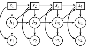
Figure 1: The independence structure of the aSLDS. Square nodes denote discrete variables, round nodes continuous variables. In the SLDS links from h to s are not normally considered.

The dynamics of the switch variables is Markovian, with transition p(st_|st₋1). The SLDS is used in many disciplines, from econometrics to machine learning (Bar-Shalom and Li, 1998; Ghahramani and Hinton, 1998; Lerner et al., 2000; Kitagawa, 1994; Kim and Nelson, 1999; Pavlovic et al., 2001). See Lerner (2002) and Zoeter (2005) for recent reviews of work.

AUGMENTEDSWITCHINGLINEARDYNAMICALSYSTEM

In this article, we will consider the more general model in which the switch st is dependent on both the previous st₋1and ht₋1. We call this an augmented Switching Linear Dynamical System2 (aSLDS), in keeping with the terminology in Lerner (2002). An equivalent probabilistic model is, as depicted in Figure (1),

p(v1:T,h1:T,s1:T) =p(v1_|h1,s1)p(h1_|s1)p(s1) T

∏

t=2

p(vt_|ht,st)p(ht_|ht₋1,st)p(st|ht−1,st−1).

The notation x1:T is shorthand for x1, . . . ,xT. The distributions are parameterized as p(vt|ht,st) =

N

N

¯h(st) +A(st)ht−1,Σh(st)

where p(h1_|s1) =

N

INFERENCE

The aim of this article is to address how to perform inference in both the SLDS and aSLDS. In par-ticular we desire the so-called filtered estimate p(ht,st|v1:t)and the smoothed estimate p(ht,st|v1:T), for any t, 1_≤t_≤T . Both exact filtered and smoothed inference in the SLDS is intractable, scaling exponentially with time (Lerner, 2002). To see this informally, consider the filtered posterior, which may be recursively computed using

p(st,ht_|v1:t) =

∑

Z

ht−1

p(st,ht_|st₋1,ht−1,vt)p(st−1,ht−1|v1:t−1). (3)

At timestep 1, p(s1,h1_|v1) =p(h1_|s1,v1)p(s1_|v1)is an indexed set of Gaussians. At time-step 2, due to the summation over the states s1, p(s2,h2|v1:2)will be an indexed set of S Gaussians; similarly at

time-step 3, it will be S2and, in general, gives rise to St−1 Gaussians. More formally, in Lauritzen and Jensen (2001), a general exact method is presented for performing stable inference in such hybrid discrete models with conditional Gaussian potentials. The method requires finding a strong junction tree which, in the SLDS case, means that the discrete variables are placed in a single cluster, resulting in exponential complexity.

The key issue in the (a)SLDS, therefore, is how to perform approximate inference in a numer-ically stable manner. Our own interest in the SLDS stems primarily from acoustic modeling, in which the time-series consists of many thousands of time-steps (Mesot and Barber, 2006; Cemgil et al., 2006). For this, we require a stable and computationally feasible approximate inference, which is also able to deal with state-spaces of high hidden dimension, H.

2. Expectation Correction

Our approach to approximate p(ht,st|v1:T)≈p(h˜ t,st|v1:T)mirrors the Rauch-Tung-Striebel (RTS) ‘correction’ smoother for the LDS (Rauch et al., 1965; Bar-Shalom and Li, 1998). Readers unfa-miliar with this approach will find a short explanation in Appendix (A), which defines the important functions LDSFORWARD and LDSBACKWARD, which we shall make use of for inference in the aSLDS. Our correction approach consists of a single Forward Pass to recursively find the filtered posterior ˜p(ht,st|v1:t), followed by a single Backward Pass to correct this into a smoothed posterior

˜

p(ht,st|v1:T). The Forward Pass we use is equivalent to Assumed Density Filtering (Alspach and Sorenson, 1972; Boyen and Koller, 1998; Minka, 2001). The main contribution of this paper is a novel form of Backward Pass, based on collapsing the smoothed posterior to a mixture of Gaussians. Unless stated otherwise, all quantities should be considered as approximations to their exact counterparts, and we will therefore usually omit the tildes˜throughout the article.

2.1 Forward Pass (Filtering)

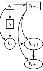
Readers familiar with Assumed Density Filtering (ADF) may wish to continue directly to Section (2.2). The basic idea is to represent the (intractable) posterior using a simpler distribution. This is then propagated forwards through time, conditioned on the new observation, and subsequently collapsed back to the tractable distribution representation—see Figure (2). Our aim is to form a recursion for p(st,ht_|v1:t), based on a Gaussian mixture approximation of p(ht_|st,v1:t). Without loss of generality, we may decompose the filtered posterior as

p(ht,st|v1:t) =p(ht|st,v1:t)p(st|v1:t).

We will first form a recursion for p(ht|st,v1:t), and discuss the switch recursion p(st|v1:t)later. The full procedure for computing the filtered posterior is presented in Algorithm (1).

The exact representation of p(ht_|st,v1:t) is a mixture with O(St_{) components. We therefore} approximate this with a smaller It-component mixture

p(ht|st,v1:t)≈p(h˜ t|st,v1:t)≡ It

∑

it=1

˜

p(ht|it,st,v1:t)p(i˜ t|st,v1:t)

where ˜p(ht_|it,st,v1:t)is a Gaussian parameterized with mean3 f(it,st)and covariance F(it,st). The Gaussian mixture weights are given by ˜p(it|st,v1:t). In the above, ˜p represent approximations to the 3. Strictly speaking, we should use the notation ft(it,st)since, for each time t, we have a set of means indexed by it,st.

st st+1

it

ht ht+1

vt+1

Figure 2: Structure of the mixture representation of the Forward Pass. Essentially, the Forward Pass defines a ‘prior’ distribution at time t which contains all the information from the variables v1:t. This prior is propagated forwards through time using the exact dynamics, conditioned on the observation, and then collapsed back to form a new prior approxima-tion at time t+1.

corresponding exact p distributions. To find a recursion for these parameters, consider

˜

p(ht+1|st+1,v1:t+1) =

∑

˜

p(ht+1,st,it|st+1,v1:t+1) =

∑

st,it

˜

p(ht+1|it,st,st+1,v1:t+1)p(s˜ t,it|st+1,v1:t+1) (4)

where each of the factors can be recursively computed on the basis of the previous filtered results (see below). However, this recursion suffers from an exponential increase in mixture components. To deal with this, we will later collapse ˜p(ht+1|st+1,v1:t+1) back to a smaller mixture. For the remainder, we drop the ˜p notation, and concentrate on computing the r.h.s of Equation (4).

EVALUATING p(ht+1|st,it,st+1,v1:t+1)

We find p(ht+1|st,it,st+1,v1:t+1)from the joint distribution p(ht+1,vt+1|st,it,st+1,v1:t), which is a Gaussian with covariance and mean elements4

Σhh=A(st+1)F(it,st)AT(st+1) +Σh(st+1), Σvv=B(st+1)ΣhhBT(st+1) +Σv(st+1)

Σvh=B(st+1)F(it,st), µv=B(st+1)A(st+1)f(it,st), µh=A(st+1)f(it,st). (5) These results are obtained from integrating the forward dynamics, Equations (1,2) over ht, using the results in Appendix (B). To find p(ht+1|st,it,st+1,v1:t+1) we may then condition p(ht+1,vt+1| st,it,st+1,v1:t)on vt+1using the results in Appendix (C)—see also Algorithm (4).

EVALUATING p(st,it|st+1,v1:t+1)

Up to a trivial normalization constant the mixture weight in Equation (4) can be found from the decomposition

Algorithm 1 aSLDS Forward Pass. Approximate the filtered posterior p(st_|v1:t)_≡ρt, p(ht|st,v1:t)≡

∑itwt(it,st)

N

require I1 =1,I2≤S,It ≤S×It−1. θt(s) =A(s),B(s),Σh(s),Σv(s),¯h(s),v(s)¯ for t >1. θ1(s) = A(s),B(s),Σ(s),Σv_{(s),µ(s),v(s)¯}

for s1←1 to S do

{f1(1,s1),F1(1,s1),pˆ_}=LDSFORWARD(0,0,v1;θ(s1))

ρ1←p(s1)pˆ end for

for t_←2 to T do for st←1 to S do

for i_←1 to It−1, and s←1 to S do

{µx|y(i,s),Σx|y(i,s),pˆ}=LDSFORWARD(ft−1(i,s),Ft−1(i,s),vt;θt(st))

p∗(st|i,s)≡ hp(st|ht−1,st−1=s)ip(ht−1|it−1=i,st−1=s,v1:t−1)

p0(st,i,s)←wt−1(i,s)p∗(st|i,s)ρt−1(s)pˆ end for

Collapse the It₋1×S mixture of Gaussians defined by µx|y,Σx|y, and weights p(i,s_|st) ∝ p0(st,i,s) to a Gaussian with It components, p(ht_|st,v1:t) _≈

∑It

it=1 p(it|st,v1:t)p(ht|st,it,v1:t). This defines the new means ft(it,st), covariances

Ft(it,st)and mixture weights wt(it,st)_≡p(it_|st,v1:t). Computeρt(st)∝ ∑i,sp0(st,i,s)

end for

normalizeρt ≡p(st|v1:t) L←L+log∑st,i,sp0(st,i,s)

end for

The first factor in Equation (6), p(vt+1|it,st,st+1,v1:t), is a Gaussian with mean µv and covariance

Σvv, as given in Equation (5). The last two factors p(it|st,v1:t) and p(st|v1:t) are given from the previous iteration. Finally, p(st+1|it,st,v1:t)is found from

p(st+1|it,st,v1:t) =hp(st+1|ht,st)ip(ht|it,st,v1:t) (7)

where_h·ip denotes expectation with respect to p. In the standard SLDS, Equation (7) is replaced by the Markov transition p(st+1|st). In the aSLDS, however, Equation (7) will generally need to be computed numerically. A simple approximation is to evaluate Equation (7) at the mean value of the distribution p(ht|it,st,v1:t). To take covariance information into account an alternative would be to draw samples from the Gaussian p(ht_|it,st,v1:t)and thus approximate the average of p(st+1|ht,st) by sampling.5

CLOSING THERECURSION

components, we numerically collapse this back to It+1Gaussians to form

p(ht+1|st+1,v1:t+1)≈ It+1

∑

it+1=1

p(ht+1|it+1,st+1,v1:t+1)p(it+1|st+1,v1:t+1).

Hence the Gaussian components and corresponding mixture weights p(it+1|st+1,v1:t+1)are defined implicitly through a numerical (Gaussian-Mixture to smaller Gaussian-Mixture) collapse procedure, for which any method of choice may be supplied. A straightforward approach that we use in our code is based on repeatedly merging low-weight components, as explained in Appendix (D).

A RECURSION FOR THESWITCHVARIABLES

A recursion for the switch variables can be found by considering

p(st+1|v1:t+1)∝

∑

it,st

p(it,st,st+1,vt+1,v1:t).

The r.h.s. of the above equation is proportional to

∑

st,it

p(vt+1|it,st,st+1,v1:t)p(st+1|it,st,v1:t)p(it|st,v1:t)p(st|v1:t)

where all terms have been computed during the recursion for p(ht+1|st+1,v1:t+1). THELIKELIHOOD p(v1:T)

The likelihood p(v1:T)may be found by recursing p(v1:t+1) =p(vt+1|v1:t)p(v1:t), where p(vt+1|v1:t) =

∑

it,st,st+1

p(vt+1|it,st,st+1,v1:t)p(st+1|it,st,v1:t)p(it|st,v1:t)p(st|v1:t).

In the above expression, all terms have been computed in forming the recursion for the filtered posterior p(ht+1,st+1|v1:t+1).

2.2 Backward Pass (Smoothing)

The main contribution of this paper is to find a suitable way to ‘correct’ the filtered posterior p(st,ht|v1:t)obtained from the Forward Pass into a smoothed posterior p(st,ht|v1:T). We initially derive this for the case of a single Gaussian representation—the extension to the mixture case is straightforward and given in Section (2.3). Our derivation holds for both the SLDS and aSLDS. We approximate the smoothed posterior p(ht|st,v1:T)by a Gaussian with mean g(st)and covariance G(st), and our aim is to find a recursion for these parameters. A useful starting point is the exact relation:

p(ht,st|v1:T) =

∑

The term p(ht_|st,st+1,v1:T)may be computed as p(ht|st,st+1,v1:T) =

Z

ht+1

p(ht,ht+1|st,st+1,v1:T) =

Z

ht+1

p(ht|ht+1,st,st+1,v1:T)p(ht+1|st,st+1,v1:T) =

Z

ht+1

p(ht_|ht+1,st,st+1,v1:t)p(ht+1|st,st+1,v1:T) (8) which is in the form of a recursion. This recursion therefore requires p(ht+1|st,st+1,v1:T), which we can write as

p(ht+1|st,st+1,v1:T)∝p(ht+1|st+1,v1:T)p(st|st+1,ht+1,v1:t). (9) The above recursions represent the exact computation of the smoothed posterior. In our approxi-mate treatment, we replace all quantities p with their corresponding approximations ˜p. A difficulty is that the functional form of ˜p(st_|st+1,ht+1,v1:t)in the approximation of Equation (9) is not squared exponential in ht+1, so that ˜p(ht+1|st,st+1,v1:T)will not be a mixture of Gaussians.6 One possibil-ity would be to approximate the non-Gaussian p(ht+1|st,st+1,v1:T)(dropping the ˜p notation) by a Gaussian (mixture) by minimizing the Kullback-Leilbler divergence between the two, or performing moment matching in the case of a single Gaussian. A simpler alternative is to make the assumption p(ht+1|st,st+1,v1:T)≈p(ht+1|st+1,v1:T), see Figure (3). This is a considerable simplification since p(ht+1|st+1,v1:T)is already known from the previous backward recursion. Under this assumption, the recursion becomes

p(ht,st|v1:T)≈

∑

p(st+1|v1:T)p(st|st+1,v1:T)hp(ht|ht+1,st,st+1,v1:t)ip(ht+1|st+1,v1:T). (10)

We call the procedure based on Equation (10) Expectation Correction (EC) since it ‘corrects’ the filtered results which themselves are formed from propagating expectations. In Appendix (E) we show how EC is equivalent to a partial Discrete-Continuous factorized approximation.

Equation (10) forms the basis of the the EC Backward Pass. However, similar to the ADF Forward Pass, the number of mixture components needed to represent the posterior in this recursion grows exponentially as we go backwards in time. The strategy we take to deal with this is a form of Assumed Density Smoothing, in which Equation (10) is interpreted as a propagated dynamics reversal, which will subsequently be collapsed back to an assumed family of distributions—see Figure (4). How we implement the recursion for the continuous and discrete factors is detailed below.7

6. In the exact calculation, p(ht+1|st,st+1,v1:T) is a mixture of Gaussians since p(st|st+1,ht+1,v1:t) =

p(st,st+1,ht+1,v1:T)/p(st+1,ht+1,v1:T) so that the mixture of Gaussians denominator p(st+1,ht+1,v1:T)cancels with the first term in Equation (9), leaving a mixture of Gaussians. However, since in Equation (9) the two terms

p(h_t+1|st+1,v1:T)and p(st|st+1,ht+1,v1:t)are replaced by approximations, this cancellation is not guaranteed. 7. Equation (10) has the pleasing form of an RTS Backward Pass for the continuous part (analogous to LDS case),

and a discrete smoother (analogous to a smoother recursion for the HMM). In the Forward-Backward algorithm for the HMM (Rabiner, 1989), the posteriorγt≡p(st|v1:T)is formed from the product ofαt≡p(st|v1:t)andβt≡

st₋1 st st+1 st+2

ht−1 ht ht+1 ht+2

vt₋1 vt vt+1 vt+2

Figure 3: Our Backward Pass approximates p(ht+1|st+1,st,v1:T) by p(ht+1|st+1,v1:T). Motivation for this is that st only influences ht+1through ht. However, ht will most likely be heavily influenced by v1:t, so that not knowing the state of st is likely to be of secondary impor-tance. The darker shaded node is the variable we wish to find the posterior state of. The lighter shaded nodes are variables in known states, and the hashed node a variable whose state is indeed known but assumed unknown for the approximation.

EVALUATINGhp(h_t|ht+1,st,st+1,v1:t)ip(ht+1|st+1,v1:T)

hp(ht_|ht+1,st,st+1,v1:t)i_{p(ht+1|st+1,v1:T)} is a Gaussian in ht, whose statistics we will now compute. First we find p(ht|ht+1,st,st+1,v1:t)which may be obtained from the joint distribution

p(ht,ht+1|st,st+1,v1:t) =p(ht+1|ht,st+1)p(ht|st,v1:t) (11)

which itself can be found using the forward dynamics from the filtered estimate p(ht|st,v1:t). The statistics for the marginal p(ht_|st,st+1,v1:t)are simply those of p(ht|st,v1:t), since st+1 carries no extra information about ht.8 The remaining statistics are the mean of ht+1, the covariance of ht+1 and cross-variance between ht and ht+1,

hht+1i=A(st+1)ft(st)

Σt+1,t+1=A(st+1)Ft(st)AT(st+1) +Σh(st+1), Σt+1,t=A(st+1)Ft(st). Given the statistics of Equation (11), we may now condition on ht+1to find p(ht|ht+1,st,st+1,v1:t). Doing so effectively constitutes a reversal of the dynamics,

ht=←−A(st,st+1)ht+1+←−η(st,st+1)

where←−A(st,st+1)and←−η(st,st+1)∼

N

condi-tioned Gaussian results in Appendix (C)—see also Algorithm (5). Averaging the reversed dynamics we obtain a Gaussian in ht forhp(ht|ht+1,st,st+1,v1:t)ip(ht+1|st+1,v1:T)with statistics

µt=←−A(st,st+1)g(st+1) +←m−(st,st+1), Σt,t=←−A(st,st+1)G(st+1)←−AT(st,st+1) +←Σ−(st,st+1).

These equations directly mirror the RTS Backward Pass, see Algorithm (5).

st st+1

it jt+1

ht ht+1

vt vt+1

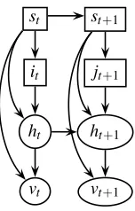
Figure 4: Structure of the Backward Pass for mixtures. Given the smoothed information at time-step t+1, we need to work backwards to ‘correct’ the filtered estimate at time t.

EVALUATING p(st|st+1,v1:T)

The main departure of EC from previous methods is in treating the term

p(st_|st+1,v1:T) =hp(st|ht+1,st+1,v1:t)ip(ht+1|st+1,v1:T). (12)

The term p(st_|ht+1,st+1,v1:t)is given by p(st|ht+1,st+1,v1:t) =

p(ht+1|st,st+1,v1:t)p(st,st+1|v1:t)

∑st0p(ht+1|s 0

t,st+1,v1:t)p(st0,st+1|v1:t)

. (13)

Here p(st,st+1|v1:t) = p(st+1|st,v1:t)p(st|v1:t), where p(st+1|st,v1:t) occurs in the Forward Pass, Equation (7). In Equation (13), p(ht+1|st+1,st,v1:t)is found by marginalizing Equation (11).

Performing the average over p(ht+1|st+1,v1:T) in Equation (12) may be achieved by any nu-merical integration method desired. Below we outline a crude approximation that is fast and often performs surprisingly well.

MEANAPPROXIMATION

A simple approximation of Equation (12) is to evaluate the integrand at the mean value of the averaging distribution. Replacing ht+1in Equation (13) by its mean gives the simple approximation

hp(st_|ht+1,st+1,v1:t)i_{p(ht+1|st+1,v1:T)}≈ 1 Z

e−12z

T

t+1(st,st+1)Σ−1(st,st+1|v1:t)zt+1(st,st+1)

p

detΣ(st,st+1|v1:t)

p(st_|st+1,v1:t) where zt+1(st,st+1)≡ hht+1|st+1,v1:Ti − hht+1|st,st+1,v1:ti and Z ensures normalization over st. This result comes simply from the fact that in Equation (12) we have a Gaussian with a mean

hht+1|st,st+1,v1:tiand covarianceΣ(st,st+1|v1:t), being the filtered covariance of ht+1given st,st+1 and the observations v1:t, which may be taken from Σhh in Equation (5). Then evaluating this Gaussian at the specific point _hht+1|st+1,v1:Ti, we arrive at the above expression. An alternative to this simple mean approximation is to sample from the Gaussian p(ht+1|st+1,v1:T), which has the potential advantage that covariance information is used.9 Other methods such as variational 9. This is a form of exact sampling since drawing samples from a Gaussian is easy. This should not be confused with

Algorithm 2 aSLDS: EC Backward Pass (Single Gaussian case I=J=1). Approximates p(st_|v1:T) and p(ht_|st,v1:T)_≡

N

GT ←FT, gT ← fT, for t_←T₋1 to 1 do

for s_←1 to S, s0_←1 to S do,

(µ,Σ)(s,s0) =LDSBACKWARD(gt+1(s0),Gt+1(s0),ft(s),Ft(s),θt+1(s0)) p(s_|s0) =_hp(st =s_|ht+1,st+1=s0,v1:t)i_{p(ht+1|st+1=s}0_,v1:T)

p(s,s0_|v1:T)← p(st+1=s0|v1:T)p(s|s0) end for

for st_←1 to S do

Collapse the mixture defined by weights p(st+1=s0|st,v1:T)∝p(st,s0|v1:T), means µ(st,s0)and covariances Σ(st,s0)to a single Gaussian. This defines the new means gt(st), covariances Gt(st).

p(st|v1:T)←∑s0p(st,s0|v1:T) end for

end for

approximations to this average (Jaakkola and Jordan, 1996) or the unscented transform (Julier and Uhlmann, 1997) may be employed if desired.

CLOSING THERECURSION

We have now computed both the continuous and discrete factors in Equation (10), which we wish to use to write the smoothed estimate in the form p(ht,st_|v1:T) =p(st_|v1:T)p(ht_|st,v1:T). The distri-bution p(ht|st,v1:T)is readily obtained from the joint Equation (10) by conditioning on st to form the mixture

p(ht|st,v1:T) =

∑

p(st+1|st,v1:T)p(ht|st,st+1,v1:T)

which may be collapsed to a single Gaussian (or mixture if desired). As in the Forward Pass, this collapse implicitly defines the Gaussian mean g(st)and covariance G(st). The smoothed posterior p(st_|v1:T)is given by

p(st_|v1:T) =

∑

p(st+1|v1:T)p(st|st+1,v1:T) =

∑

st+1

p(st+1|v1:T)hp(st|ht+1,st+1,v1:t)i_{p(ht+1|st+1,v1:T)}. (14)

The algorithm for the single Gaussian case is presented in Algorithm (2).

NUMERICALSTABILITY

Numerical stability is a concern even in the LDS, and the same is to be expected for the aSLDS.

Since the LDS recursions LDSFORWARD and LDSBACKWARD are embedded within the EC

RELAXINGEC

The conditional independence assumption p(ht+1|st,st+1,v1:T)≈ p(ht+1|st+1,v1:T) is not strictly necessary in EC. We motivate it by computational simplicity, since finding an appropriate moment matching approximation of p(ht+1|st,st+1,v1:T)in Equation (9) requires a relatively expensive non-Gaussian integration. If we therefore did treat p(ht+1|st,st+1,v1:T) more correctly, the central as-sumption in this relaxed version of EC would be a collapse to a mixture of Gaussians (the additional computation of Equation (12) may usually be numerically evaluated to high precision). Whilst we did not do so, implementing this should not give rise to numerical instabilities since no potential divisions are required, merely the estimation of moments. In the experiments presented here, we did not pursue this option, since we believe that the effect of this conditional independence assumption is relatively weak.

INCONSISTENCIES IN THE APPROXIMATION

The recursion Equation (8), upon which EC depends, makes use of the Forward Pass results, and a subtle issue arises about possible inconsistencies in the Forward and Backward approxi-mations. For example, under the conditional independence assumption in the Backward Pass, p(hT_|sT₋1,sT,v1:T)≈ p(hT|sT,v1:T), which is in contradiction to Equation (5) which states that the approximation to p(hT|sT−1,sT,v1:T)will depend on sT−1. Similar contradictions occur also for the relaxed version of EC. Such potential inconsistencies arise because of the approximations made, and should not be considered as separate approximations in themselves. Furthermore, these incon-sistencies will most likely be strongest at the end of the chain, t_≈T , since only then is Equation (8) in direct contradiction to Equation (5). Such potential inconsistencies arise since EC is not founded on a consistency criterion, unlike EP—see Section (3)—but rather an approximation of the exact recursions. Our experience is that compared to EP, which attempts to ensure consistency based on multiple sweeps through the graph, such inconsistencies are a small price to pay compared to the numerical stability advantages of EC.

2.3 Using Mixtures in the Backward Pass

The extension to the mixture case is straightforward, based on the representation

p(ht|st,v1:T)≈ Jt

∑

jt=1

p(ht|st,jt,v1:T)p(jt|st,v1:T).

Analogously to the case with a single component,

p(ht,st_|v1:T) =

∑

p(st+1|v1:T)p(jt+1|st+1,v1:T)p(ht|jt+1,st+1,it,st,v1:T)

· hp(it,st_|ht+1,jt+1,st+1,v1:t)ip(ht+1|jt+1,st+1,v1:T).

The average in the last line of the above equation can be tackled using the same techniques as outlined in the single Gaussian case. To approximate p(ht|jt+1,st+1,it,st,v1:T)we consider this as the marginal of the joint distribution

Algorithm 3 aSLDS: EC Backward Pass. Approximates p(st_|v1:T) and p(ht_|st,v1:T) _≡

∑Jt

jt=1ut(jt,st)

N

routine needs the results from Algorithm (1). GT ←FT, gT ← fT, uT←wT (*)

for t_←T₋1 to 1 do

for s_←1 to S, s0_←1 to S, i_←1 to It, j0←1 to Jt+1do

(µ,Σ)(i,s,j0,s0) =LDSBACKWARD(g_t+1(j0,s0),Gt+1(j0,s0),ft(i,s),Ft(i,s),θt+1(s0)) p(i,s_|j0,s0) =_hp(st=s,it=i_|ht+1,st+1=s0,jt+1= j0,v1:t)ip(ht+1|st+1=s0,jt+1=j0,v1:T)

p(i,s,j0,s0_|v1:T)←p(st+1=s0|v1:T)ut+1(j0,s0)p(i,s|j0,s0) end for

for st_←1 to S do

Collapse the mixture defined by weights p(it =i,st+1 = s0,jt+1 = j0|st,v1:T) ∝ p(i,st,j0,s0_|v1:T), means µ(it,st,j0,s0)and covariancesΣ(it,st,j0,s0)to a mixture with Jt components. This defines the new means gt(jt,st), covariances Gt(jt,st)and mix-ture weights ut(jt,st).

p(st|v1:T)←∑it,j0,s0p(it,st,j0,s0|v1:T)

end for end for

(*) If JT <IT then the initialization is formed by collapsing the Forward Pass results at time T to JT components.

As in the case of a single mixture, the problematic term is p(ht+1|it,st,jt+1,st+1,v1:T). Analogously to before, we may make the assumption

p(ht+1|it,st,jt+1,st+1,v1:T)≈p(ht+1|jt+1,st+1,v1:T)

meaning that information about the current switch state st,it is ignored.10 We can then form p(ht|st,v1:T) =

∑

it,jt+1,st+1

p(it,jt+1,st+1|st,v1:T)p(ht|it,st,jt+1,st+1,v1:T).

This mixture can then be collapsed to smaller mixture using any method of choice, to give

p(ht|st,v1:T)≈ Jt

∑

jt=1

p(ht|jt,st,v1:T)p(jt|st,v1:T)

The collapse procedure implicitly defines the means g(jt,st)and covariances G(jt,st)of the smoothed approximation. A recursion for the switches follows analogously to the single component Backward Pass. The resulting algorithm is presented in Algorithm (3), which includes using mixtures in both Forward and Backward Passes. Note that if JT <IT, an extra initial collapse is required of the IT component Forward Pass Gaussian mixture at time T to JT components.

EC has time complexity O(S2_{IJK) where S are the number of switch states, I and J are the} number of Gaussians used in the Forward and Backward passes, and K is the time to compute the exact Kalman smoother for the system with a single switch state.

3. Relation to Other Methods

Approximate inference in the SLDS is a long-standing research topic, generating an extensive liter-ature. See Lerner (2002) and Zoeter (2005) for reviews of previous work. A brief summary of some of the major existing approaches follows.

Assumed Density Filtering Since the exact filtered estimate p(ht_|st,v1:t)is an (exponentially large) mixture of Gaussians, a useful remedy is to project at each stage of the recursion Equation (3) back to a limited set of K Gaussians. This is a Gaussian Sum Approximation (Alspach and Sorenson, 1972), and is a form of Assumed Density Filtering (ADF) (Minka, 2001). Simi-larly, Generalized Pseudo Bayes2 (GPB2) (Bar-Shalom and Li, 1998) also performs filtering by collapsing to a mixture of Gaussians. This approach to filtering is also taken in Lerner et al. (2000) which performs the collapse by removing spatially similar Gaussians, thereby retaining diversity.

Several smoothing approaches directly use the results from ADF. The most popular is Kim’s method, which updates the filtered posterior weights to form the smoother (Kim, 1994; Kim and Nelson, 1999). In both EC and Kim’s method, the approximation

p(ht+1|st,st+1,v1:T)≈p(ht+1|st+1,v1:T), is used to form a numerically simple Backward Pass. The other approximation in EC is to numerically compute the average in Equation (14). In Kim’s method, however, an update for the discrete variables is formed by replacing the re-quired term in Equation (14) by

hp(st|ht+1,st+1,v1:t)ip(ht+1|st+1,v1:T)≈p(st|st+1,v1:t). (15)

This approximation11decouples the discrete Backward Pass in Kim’s method from the con-tinuous dynamics, since p(st|st+1,v1:t)∝ p(st+1|st)p(st|v1:t)/p(st+1|v1:t) can be computed simply from the filtered results alone (the continuous Backward Pass in Kim’s method, how-ever, does depend on the discrete Backward Pass). The fundamental difference between EC and Kim’s method is that the approximation (15) is not required by EC. The EC Backward Pass therefore makes fuller use of the future information, resulting in a recursion which in-timately couples the continuous and discrete variables. The resulting effect on the quality of the approximation can be profound, as we will see in the experiments.

Kim’s smoother corresponds to a potentially severe loss of future information and, in general, cannot be expected to improve much on the filtered results from ADF. The more recent work of Lerner et al. (2000) is similar in spirit to Kim’s method, whereby the contribution from the continuous variables is ignored in forming an approximate recursion for the smoothed p(st|v1:T). The main difference is that for the discrete variables, Kim’s method is based on a correction smoother (Rauch et al., 1965), whereas Lerner’s method uses a Belief Propagation style Backward Pass (Jordan, 1998). Neither method correctly integrates information from the continuous variables. How to form a recursion for a mixture approximation which does not ignore information coming through the continuous hidden variables is a central contribution of our work.

Kitagawa (1994) used a two-filter method in which the dynamics of the chain are reversed. Essentially, this corresponds to a Belief Propagation method which defines a Gaussian sum

EC Relaxed EC EP Kim

Mixture Collapsing to Single x

Mixture Collapsing to Mixture x x x

Cond. Indep. p(ht+1|st,st+1,v1:T)≈p(ht+1|st+1,v1:T) x x Approx. of p(st|st+1,v1:T), average Equation (12) x x

Kim’s Backward Pass x

Mixture approx. of p(h_t+1|st,st+1,v1:T), Equation (9) x

Table 1: Relation between methods. In the EC methods, the mean approximation may be replaced by an essentially exact Monte Carlo approximation to Equation (12). EP refers to the Single Gaussian approximation in Heskes and Zoeter (2002). In the case of using Relaxed EC with collapse to a single Gaussian, EC and EP are not equivalent, since the underlying recursions on which the two methods are based are fundamentally different.

approximation for p(vt+1:T|ht,st). However, since this is not a density in ht,st, but rather a conditional likelihood, formally one cannot treat this using density propagation methods. In Kitagawa (1994), the singularities resulting from incorrectly treating p(vt+1:T|ht,st) as a density are heuristically finessed.

Expectation Propagation EP (Minka, 2001), as applied to the SLDS, corresponds to an approxi-mate implementation of Belief Propagation12 (Jordan, 1998; Heskes and Zoeter, 2002). EP is the most sophisticated rival to Kim’s method and EC, since it makes the least assumptions. For this reason, we’ll explain briefly how EP works. Unlike EC, which is based on an ap-proximation of the exact filtering and smoothing recursions, EP is based on a consistency criterion.

First, let’s simplify the notation, and write the distribution as p=∏_tφ(xt−1,vt−1,xt,vt), where xt≡ht⊗st, andφ(xt−1,vt−1,xt,vt)≡p(xt|xt−1)p(vt|xt). EP defines ‘messages’ρ,λ13which contain information from past and future observations respectively.14 Explicitly, we define

ρt(xt)∝p(xt|v1:t) to represent knowledge about xt given all information from time 1 to t. Similarly,λt(xt) represents knowledge about state xt given all observations from time T to time t+1. In the sequel, we drop the time suffix for notational clarity. We define λ(xt) implicitly through the requirement that the marginal smoothed inference is given by

p(xt|v1:T)∝ ρ(xt)λ(xt). (16)

Hence λ(xt)∝ p(vt+1:T|xt,v1:t) = p(vt+1:T|xt) and represents all future knowledge about p(xt|v1:T). From this

p(xt₋1,xt|v1:T)∝ ρ(xt−1)φ(xt−1,vt−1,xt,vt)λ(xt). (17) 12. Non-parametric belief propagation (Sudderth et al., 2003), which performs approximate inference in general contin-uous distributions, is also related to EP applied to the aSLDS, in the sense that the messages cannot be represented easily, and are approximated by mixtures of Gaussians.

13. These correspond to theαandβmessages in the Hidden Markov Model framework (Rabiner, 1989).

Taking the above equation as a starting point, we have

p(xt|v1:T)∝

Z

xt−1

ρ(xt−1)φ(xt−1,vt−1,xt,vt)λ(xt).

Consistency with Equation (16) requires (neglecting irrelevant scalings)

ρ(xt)λ(xt)∝

Z

xt−1

ρ(xt₋1)φ(xt−1,vt−1,xt,vt)λ(xt).

Similarly, we can integrate Equation (17) over xt to get the marginal at time xt₋1which, by consistency, should be proportional toρ(xt−1)λ(xt−1). Hence

ρ(xt)∝

R

xt−1ρ(xt−1)φ(xt−1,xt)λ(xt)

λ(xt)

,λ(xt−1)∝

R

xtρ(xt−1)φ(xt−1,xt)λ(xt)

ρ(xt−1)

(18)

where the divisions can be interpreted as preventing over-counting of messages. In an exact implementation, the common factors in the numerator and denominator cancel. EP addresses the fact that λ(xt) is not a distribution by using Equation (18) to form the projection (or ‘collapse’). In the numerator, R

xt−1ρ(xt−1)φ(xt−1,xt)λ(xt) and

R

xtρ(xt−1)φ(xt−1,xt)λ(xt)

represent p(xt_|v1:T) and p(xt₋1|v1:T). Since these are distributions (an indexed mixture of Gaussians in the SLDS), they may be projected/collapsed to a single indexed Gaussian. The update for the ρ message is then found from division by the λ potential, and vice versa. In EP the explicit division of potentials only makes sense for members of the exponential family. More complex methods could be envisaged in which, rather than an explicit divi-sion, the new messages are defined by minimizing some measure of divergence between

ρ(xt)λ(xt)andR

xt−1ρ(xt−1)φ(xt−1,xt)λ(xt), such as the Kullback-Leibler divergence. In this

way, non-exponential family approximations (such as mixtures of Gaussians) may be consid-ered. Whilst this is certainly feasible, it is somewhat unattractive computationally since this would require for each time-step an expensive minimization.

For the single Gaussian case, in order to perform the division, the potentials in the numerator and denominator are converted to their canonical representations. To form the ρ update, the result of the division is then reconverted back to a moment representation. The resulting recursions, due to the approximation, are no longer independent and Heskes and Zoeter (2002) show that using more than a single Forward and Backward sweep often improves on the quality of the approximation. This coupling is a departure from the exact recursions, which should remain independent.

which is numerically unstable due to conversion between moment and canonical representa-tions, and Lauritzen and Jensen (2001), which improves stability by avoiding using canonical parameterizations.

Variational Methods Ghahramani and Hinton (1998) used a variational method which approxi-mates the joint distribution p(h1:T,s1:T_|v1:T) rather than the marginal p(ht,st_|v1:T)—related work is presented in Lee et al. (2004). This is a disadvantage when compared to other methods that directly approximate the marginal. The variational methods are nevertheless potentially attractive since they are able to exploit structural properties of the distribution, such as a fac-tored discrete state-transition. In this article, we concentrate on the case of a small number of states S and hence will not consider variational methods further here.15

Sequential Monte Carlo (Particle Filtering) These methods form an approximate implementation of Equation (3), using a sum of delta functions to represent the posterior—see, for example, Doucet et al. (2001). Whilst potentially powerful, these non-analytic methods typically suffer in high-dimensional hidden spaces since they are often based on naive importance sampling, which restricts their practical use. ADF is generally preferential to Particle Filtering, since in ADF the approximation is a mixture of non-trivial distributions, which is better at capturing the variability of the posterior. Rao-Blackwellized Particle Filters (Doucet et al., 2000) are an attempt to alleviate the difficulty of sampling in high-dimensional state spaces by explicitly integrating over the continuous state.

Non-Sequential Monte Carlo

For fixed switches s1:T, p(v1:T_|s1:T) is easily computable since this is just the likelihood of an LDS. This observation raises the possibility of sampling from the posterior p(s1:T|v1:T)∝ p(v1:T_|s1:T)p(s1:T)directly. Many possible sampling methods could be applied in this case, and the most immediate is Gibbs sampling, in which a sample for each t is drawn from p(st|s_\t,v1:T)—see Neal (1993) for a general reference and Carter and Kohn (1996) for an application to the SLDS. This procedure may work well in practice provided that the initial setting of s1:Tis in a region of high probability mass—otherwise, sampling by such individual coordinate updates may be extremely inefficient.

4. Experiments

Our experiments examine the stability and accuracy of EC against several other methods on long time-series. In addition, we will compare the absolute accuracy of EC as a function of the number of mixture components on a short time-series, where exact inference may be explicitly evaluated.

Testing EC in a problem with a reasonably long temporal sequence, T , is important since nu-merical stabilities may not be apparent in time-series of just a few time-steps. To do this, we sequentially generate hidden states ht,st and observations vt from a given model. Then, given only the parameters of the model and the observations (but not any of the hidden states), the task is to infer p(ht|st,v1:T)and p(st|v1:T). Since the exact computation is exponential in T , a formally exact evaluation of the method is infeasible. A simple alternative is to assume that the original sam-ple states s1:T are the ‘correct’ inferred states, and compare our most probable posterior smoothed

0 10 20 30 40 50 60 70 80 90 100 −80 −60 −40 −20 0 20 40 60 80

(a) Easy problem

0 10 20 30 40 50 60 70 80 90 100 −200 −150 −100 −50 0 50 100 150

(b) Hard problem

Figure 5: SLDS: Throughout, S=2, V =1 (scalar observations), T =100, with zero output bias. A(s) =0.9999_∗orth(randn(H,H)), B(s) =randn(V,H), ¯vt ≡0, ¯h1=10∗randn(H,1), ¯ht>1=0,Σh1=IH, p1=uniform. The figures show typical examples for each of the two problems: (a) Easy problem. H=3,Σh(s) =IH, Σv(s) =0.1IV, p(st+1|st)∝1S×S+IS. (b) Hard problem. H=30,Σv(s) =30IV,Σh(s) =0.01IH, p(st+1|st)∝1S×S.

0 10 20 0 200 400 600 800 1000 PF

0 10 20 RBPF

0 10 20 EP

0 10 20 ADFS

0 10 20 KimS

0 10 20 ECS

0 10 20 ADFM

0 10 20 KimM

0 10 20 ECM

0 10 20 Gibbs

Figure 6: SLDS ‘Easy’ problem: The number of errors in estimating a binary switch p(st_|v1:T)over a time series of length T=100. Hence 50 errors corresponds to random guessing. Plotted are histograms of the errors over 1000 experiments. The histograms have been cutoff at 20 errors in order to improve visualization. (PF) Particle Filter. (RBPF) Rao-Blackwellized PF. (EP) Expectation Propagation. (ADFS) Assumed Density Filtering using a Single Gaussian. (KimS) Kim’s smoother using the results from ADFS. (ECS) Expectation Correction using a Single Gaussian (I=J=1). (ADFM) ADF using a multiple of I=4 Gaussians. (KimM) Kim’s smoother using the results from ADFM. (ECM) Expectation Correction using a mixture with I=J=4 components. In Gibbs sampling, we use the initialization from ADFM.

estimates arg maxstp(st|v1:T)with the assumed correct sample st.

16 _{We look at two sets of} experi-ments, one for the SLDS and one for the aSLDS. In both cases, scalar observations are used so that the complexity of the inference problem can be visually assessed.

0 25 50 75 0 200 400 600 800 1000

PF

0 25 50 75 RBPF

0 25 50 75 EP

0 25 50 75 ADFS

0 25 50 75 KimS

0 25 50 75 ECS

0 25 50 75 ADFM

0 25 50 75 KimM

0 25 50 75 ECM

0 25 50 75 Gibbs

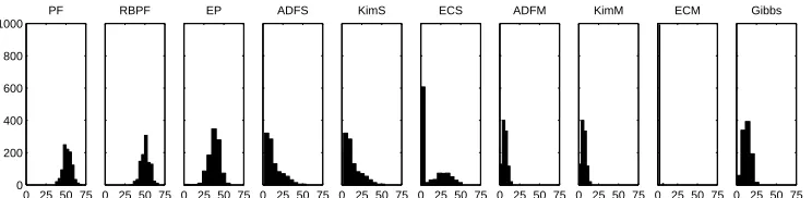
Figure 7: SLDS ‘Hard’ problem: The number of errors in estimating a binary switch p(st_|v1:T)over a time series of length T=100. Hence 50 errors corresponds to random guessing. Plotted are histograms of the errors over 1000 experiments.

SLDS EXPERIMENTS

We chose experimental conditions that, from the viewpoint of classical signal processing, are dif-ficult, with changes in the switches occurring at a much higher rate than the typical frequencies in the signal. We consider two different toy SLDS experiments : The ‘easy’ problem corresponds to a low hidden dimension, H =3, with low observation noise; The ‘hard’ problem corresponds to a high hidden dimension, H =30, and high observation noise. See Figure (5) for details of the experimental setup.

We compared methods using a single Gaussian, and methods using multiple Gaussians, see Fig-ure (6) and FigFig-ure (7). For EC we use the mean approximation for the numerical integration of Equation (12). For the Particle Filter 1000 particles were used, with Kitagawa re-sampling (Kita-gawa, 1996). For the Rao-Blackwellized Particle Filter (Doucet et al., 2000), 500 particles were used, with Kitagawa re-sampling. We included the Particle Filter merely for a point of comparison with ADF, since they are not designed to approximate the smoothed estimate.

An alternative MCMC procedure is to perform Gibbs sampling of p(s1:T_|v1:T)using p(st_|s_\t,v1:T)∝ p(v1:T_|s1:T)p(s1:T), where p(v1:T_|s1:T)is simply the likelihood of an LDS—see for example Carter and Kohn (1996).17 We initialize the state s1:T by using the most likely states st from the filtered results using a Gaussian mixture (ADFM), and then swept forwards in time, sampling from the state p(st_|s_\t,v1:T)until the end of the chain. We then reversed direction, sampling from time T back to time 1, and continued repeating this procedure 100 times, with the mean over the last 80 sweeps used as the posterior mean approximation. This procedure is expensive since each sample requires computing the likelihood of an LDS defined on the whole time-series. The procedure therefore scales with GT2where G is the number of sweeps over the time series. Despite using a reasonable initialization, Gibbs sampling struggles to improve on the filtered results.

We found that EP was numerically unstable and often struggled to converge. To encourage convergence, we used the damping method in Heskes and Zoeter (2002), performing 20 iterations with a damping factor of 0.5. The disappointing performance of EP is most likely due to conflicts

0 10 20 30 40 50 60 0

200 400 600 800 1000

PF

0 10 20 30 40 50 60

ADFS

0 10 20 30 40 50 60

ECS

0 10 20 30 40 50 60

ADFM

0 10 20 30 40 50 60

ECM

Figure 8: aSLDS: Histogram of the number of errors in estimating a binary switch p(st_|v1:T)over a time series of length T=100. Hence 50 errors corresponds to random guessing. Plotted are histograms of the errors over 1000 experiments. Augmented SLDS results. ADFM used I=4 Gaussians, and ECM used I =J=4 Gaussians. We used 1000 samples to approximate Equation (12).

I 1 4 4 16 16 64 64 256 256

J 1 1 4 1 16 1 64 1 256

error 0.0989 0.0624 0.0365 0.0440 0.0130 0.0440 4.75e-4 0.0440 3.40e-8

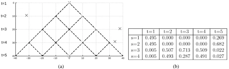
Table 2: Errors in approximating the states for the multi-path problem, see Figure (9). The mean absolute deviation_|pec(st_|v1:T)₋pexact(st_|v1:T)_|averaged over the S=4 states of st and over the times t=1, . . . ,5, computed for different numbers of mixture components in EC. The mean approximation of Equation (12) is used. The exact computation uses ST−1=256 mixtures.

resulting from numerical instabilities introduced by the frequent conversions between moment and canonical representations.

The various algorithms differ widely in performance, see Figures (6,7). Not surprisingly, the best filtered results are given using ADF, since this is better able to represent the variance in the filtered posterior than the sampling methods. Unlike Kim’s method, EC makes good use of the future information to clean up the filtered results considerably. One should bear in mind that both EC, Kim’s method and the Gibbs initialization use the same ADF results. These results show that EC may dramatically improve on Kim’s method, so that the small amount of extra work in making a numerical approximation of p(st_|st+1,v1:T), Equation (12), may bring significant benefits. AUGMENTEDSLDS EXPERIMENTS

In Figure (8), we chose a simple two state S=2 transition distribution p(st+1=1|st,ht) =σ hTtw(st)

−40 −30 −20 −10 0 10 20 30 40 0

10

20

30

40

t=1

t=2

t=3

t=4

t=5

(a) (b)

Figure 9: (a) The multi-path problem. The particle starts from(0,0)at time t=1. Subsequently, at each time-point, either the vector(10,10) (corresponding to states s=1 and s=3) or(₋10,10)(corresponding to states s=2 and s=4), is added to the hidden dynamics, perturbed by a small amount of noise,Σh=0.1. The observations are v=h+ηv_{(s). For} states s=1,2 the observation noise is small,Σv=0.1I, but for s=3,4 the noise in the horizontal direction has variance 1000. The visible observations are given by the x’. The true hidden states are given by ‘+’. (b) The exact smoothed state posteriors pexact(st_|v1:T) computed by enumerating all paths (given by the dashed lines).

we set to be block diagonal. The first 2_×2 block is set to 0.9999R_θ, where R_θ is a 2_×2 rotation matrix with angleθchosen uniformly from 0 to 1 radians. This means that st+1is dependent on the first two components of htwhich are rotating at a restricted rate. The remaining H₋2_×H₋2 block of A(s)is chosen as (using MATLAB notation) 0.9999_∗orth(rand(H₋2)), which means a scaled randomly chosen orthogonal matrix. Throughout, S=2, V =1, H=30, T=100, with zero output bias. Using partly MATLAB notation, B(s) =randn(V,H), ¯vt ≡0, ¯h1=10∗randn(H,1), ¯ht>1=0,

Σh

1=IH, p1=uniform.Σv=30IV,Σh=0.1IH.

We compare EC only against Particle Filters using 1000 particles, since other methods would require specialized and novel implementations. In ADFM, I =4 Gaussians were used, and for ECM, I=J=4 Gaussians were used. Looking at the results in Figure (8), we see that EC performs well, with some improvement in using the mixture representation I,J=4 over a single Gaussian I=J=1. The Particle Filter most likely failed since the hidden dimension is too high to be explored well with only 1000 particles.

EFFECT OFUSINGMIXTURES

are several paths that might plausibly have been taken to give rise to the observations. The accuracy with which EC predicts the exact smoothed posterior is given in Table (2). For this problem we see that both the number of Forward (I) and Backward components (J) affects the accuracy of the approximation, generally with improved accuracy as the number of mixture components increases. For a ‘perfect’ approximation method, one would expect that when I=J=ST−1=256, then the approximation should become exact. The small error for this case in Table (2) may arise for several reasons: the extra independence assumption used in EC, or the simple mean approximation used to compute Equation (12), or numerical roundoff. However, at least in this case, the effect of these assumptions on the performance is very small.

5. Discussion

Expectation Correction is a novel form of Backward Pass which makes less approximations than the widely used approach from Kim (1994). In Kim’s method, potentially important future information channeled through the continuous hidden variables is lost. EC, along with Kim’s method, makes the additional assumption p(ht+1|st,st+1,v1:T)≈p(ht+1|st+1,v1:T). However, our experience is that this assumption is rather mild, since the state of ht+1will be most heavily influenced by its immediate parent st+1.

Our approximation is based on the idea that, although exact inference will consist of an expo-nentially large number of mixture components, due to the forgetting which commonly occurs in Markovian models, a finite number of mixture components may provide a reasonable approxima-tion. In tracking situations where the visible information is (temporarily) not enough to specify accurately the hidden state, then representing the posterior p(ht_|st,v1:T)using a mixture of Gaus-sians may improve results significantly. Clearly, in systems with very long correlation times our method may require too many mixture components to produce a satisfactory result, although we are unaware of other techniques that would be able to cope well in that case.

We hope that the straightforward ideas presented here may help facilitate the practical appli-cation of dynamic hybrid networks to machine learning and related areas. Whilst models with Gaussian emission distributions such as the SLDS are widespread, the extension of this method to non-Gaussian emissions p(vt|ht,st)would clearly be of considerable interest.

Software for Expectation Correction for this augmented class of Switching Linear Gaussian models is available fromwww.idiap.ch/_∼barber.

Acknowledgments

Algorithm 4 LDS Forward Pass. Compute the filtered posteriors p(ht|v1:t) ≡

N

θ1=A,B,Σ,Σv,µ,v, where¯ Σ and µ are the prior covariance and mean of h. The log-likelihood L=log p(v1:T)is also returned.

F0←0, f0←0, L←0 for t_←1,T do

{ft,Ft,pt_}=LDSFORWARD(ft₋1,Ft−1,vt;θt) L_←L+log pt

end for

functionLDSFORWARD( f,F,v;θ)

Compute jointp(ht,vt|v1:t₋1):

µh←A f+¯h, µv←Bµh+v¯

Σhh←AFAT+Σh, Σvv←BΣhhBT+Σv, Σvh←BΣhh

Findp(ht|v1:t)by conditioning:

f0_←µh+Σ_vhTΣ−vv1(v−µv), F0←Σhh−ΣT_vhΣ−vv1Σvh

Computep(vt|v1:t−1):

p0_←exp

−12(v−µv)

T_Σ−1 vv (v−µv)

/√det 2πΣvv return f0,F0,p0

end function

Appendix A. Inference in the LDS

The LDS is defined by Equations (1,2) in the case of a single switch S=1. The LDS Forward

and Backward passes define the important functions LDSFORWARD and LDSBACKWARD, which

we shall make use of for inference in the aSLDS.

FORWARDPASS(FILTERING)

The filtered posterior p(ht_|v1:t)is a Gaussian which we parameterize with mean ft and covariance Ft. These parameters can be updated recursively using p(ht|v1:t)∝p(ht,vt|v1:t₋1), where the joint distribution p(ht,vt|v1:t−1)has statistics (see Appendix (B))

µh=A ft₋1+¯h, µv=Bµh+v¯

Σhh=AFt−1AT+Σh, Σvv=BΣhhBT+Σv, Σvh=BΣhh.

We may then find p(ht|v1:t)by conditioning p(ht,vt|v1:t−1)on vt, see Appendix (C). This gives rise to Algorithm (4).

BACKWARDPASS

The smoothed posterior p(ht|v1:T)≡

N

Z

ht+1

p(ht_|ht+1,v1:T)p(ht+1|v1:T) =

Z

ht+1

p(ht_|ht+1,v1:t)p(ht+1|v1:T) where p(ht|ht+1,v1:t)may be obtained from the joint distribution

Algorithm 5 LDS Backward Pass. Compute the smoothed posteriors p(ht_|v1:T). This requires the filtered results from Algorithm (4).

GT _←FT, gT ← fT for t_←T₋1,1 do

{gt,Gt_}=LDSBACKWARD(gt+1,Gt+1,ft,Ft;θt+1)

end for

functionLDSBACKWARD(g,G,f,F;θ)

µh_←A f+¯h, Σh0_h0 ←AFAT+Σh, Σ_h0_h←AF

←_Σ−

←Ft−ΣT_h0_hΣ−_h01_h0Σh0h, ←−A ←ΣT_h0hΣ−_h01_h0, ←m−← f−←A µh−

g0_←←−A g+←m ,− G0_←←−A G←A−T₊←Σ−

return g0,G0 end function

which itself can be obtained by forward propagation from p(ht_|v1:t). Conditioning Equation (19) to find p(ht|ht+1,v1:t)effectively reverses the dynamics,

ht=←At−ht+1+←η−t

where←A−t and←−ηt∼

N

gt=←A−tgt+1+←m−t, Gt =←A−tGt+1←A−tT+←Σ−t.

This Backward Pass is given in Algorithm (5). For parameter learning of the A matrix, the smoothed statistichthT_t+1is required. Using the above formulation, this is given by←At−Gt+1+hhti

hT_t+1. This is much simpler than the standard expressions cited in Shumway and Stoffer (2000) and Roweis and Ghahramani (1999).

Appendix B. Gaussian Propagation

Let y be linearly related to x through y=Mx+η, where η_∼

N

N

xp(y|x)p(x)is a Gaussian with mean Mµx+µ and covariance MΣxMT+Σ. Appendix C. Gaussian Conditioning

For a joint Gaussian distribution over the vectors x and y with means µx, µyand covariance elements

Σxx,Σxy,Σyy, the conditional p(x|y) is a Gaussian with mean µx+ΣxyΣ−yy1(y−µy) and covariance

Σxx−ΣxyΣ−yy1Σyx.

Appendix D. Collapsing Gaussians

First, we describe how to collapse a mixture to a single Gaussian: We may collapse a mix-ture of Gaussians p(x) =∑ipi

N

∑ipi Σi+µiµTi

−µµT_.

To collapse a mixture to a K-component mixture we retain the K₋1 Gaussians with the largest mixture weights—the remaining N₋K Gaussians are simply merged to a single Gaussian using the above method. The alternative of recursively merging the two Gaussians with the lowest mixture weights gave similar experimental performance.

More sophisticated methods which retain some spatial information would clearly be potentially useful. The method presented in Lerner et al. (2000) is a suitable approach which considers remov-ing Gaussians which are spatially similar (and not just low-weight components), thereby retainremov-ing diversity over the possible solutions.

Appendix E. The Discrete-Continuous Factorization Viewpoint

An alternative viewpoint is to proceed analogously to the Rauch-Tung-Striebel correction method for the LDS (Grewal and Andrews, 1993):

p(ht,st_|v1:T) =

∑

Z

ht+1

p(st,ht,ht+1,st+1|v1:T) =

∑

st+1

p(st+1|v1:T)

Z

ht+1

p(ht,st|ht+1,st+1,v1:t)p(ht+1|st+1,v1:T) =

∑

st+1

p(st+1|v1:T)hp(ht|ht+1,st+1,st,v1:t)p(st|ht+1,st+1,v1:t)i

≈

∑

st+1

p(st+1|v1:T)hp(ht|ht+1,st+1,st,v1:t)ihp(st|st+1,v1:T)i

| {z }

p(st|st+1,v1:T)

(20)

where angled brackets_h·idenote averages with respect to p(ht+1|st+1,v1:T). Whilst the factorized approximation in Equation (20) may seem severe, by comparing Equations (20) and (10) we see that it is equivalent to the apparently milder assumption p(ht+1|st,st+1,v1:T)≈p(ht+1|st+1,v1:T). Hence this factorized approximation is equivalent to the ‘standard’ EC approach in which the dependency on stis dropped.

References

D. L. Alspach and H. W. Sorenson. Nonlinear bayesian estimation using gaussian sum approxima-tions. IEEE Transactions on Automatic Control, 17(4):439–448, 1972.

Y. Bar-Shalom and Xiao-Rong Li. Estimation and Tracking : Principles, Techniques and Software. Artech House, Norwood, MA, 1998.

X. Boyen and D. Koller. Tractable inference for complex stochastic processes. In Proceedings of the 14th Conference on Uncertainty in Artificial Intelligence—UAI 1998, pages 33–42. Morgan Kaufmann, 1998.