Nonlinear Boosting Projections for Ensemble Construction

(1)

Nonlinear Boosting Projections for Ensemble Construction

Nicol´as Garc´ıa-Pedrajas [email protected]

Department of Computing and Numerical Analysis University of C´ordoba

C´ordoba, Spain

C´esar Garc´ıa-Osorio [email protected]

Department of Civil Engineering University of Burgos

Burgos, Spain

Colin Fyfe [email protected]

School of Computing University of Paisley Paisley, United Kingdom

Editor: Dale Schuurmans

Abstract

In this paper we propose a novel approach for ensemble construction based on the use of nonlinear projections to achieve both accuracy and diversity of individual classifiers. The proposed approach combines the philosophy of boosting, putting more effort on difficult instances, with the basis of the random subspace method. Our main contribution is that instead of using a random subspace, we construct a projection taking into account the instances which have posed most difficulties to previous classifiers. In this way, consecutive nonlinear projections are created by a neural network trained using only incorrectly classified instances. The feature subspace induced by the hidden layer of this network is used as the input space to a new classifier. The method is compared with bagging and boosting techniques, showing an improved performance on a large set of 44 problems from the UCI Machine Learning Repository. An additional study showed that the proposed approach is less sensitive to noise in the data than boosting methods.

Keywords: classifier ensembles, boosting, neural networks, nonlinear projections

1. Introduction

An ensemble of classifiers consists of a combination of different classifiers, homogeneous or het-erogeneous, to jointly perform a classification task. Ensemble construction is one of the fields of Artificial Intelligence that is receiving most research attention, mainly due to the significant performance improvements over single classifiers that have been reported with ensemble methods (Breiman, 1996a; Kohavi and Kunz, 1997; Bauer and Kohavi, 1999; Webb, 2000; Garc´ıa-Pedrajas et al., 2005).

(2)

The task is to find a definition for the unknown function, f(x), given the set of training instances. In a classifier ensemble framework we have a set of classifiers =_{C1,C2, . . . ,Cm}, each classifier performing a mapping of an instance vector x_∈ D onto the set of labels Y =_{1, . . . ,K_}. The design of classifier ensembles must face two main tasks: constructing the individuals classifiers,

Ci, and developing a combination rule that finds a class label for x based on the outputs of the

classifiers_{C1(x),C2(x), . . . ,Cm(x)}. This paper is devoted to the first problem, the combination of the classifiers is being done with a simple majority voting scheme.

For more detailed descriptions of ensembles the reader is referred to other reviews: Dietterich (2000b), Webb (2000), Dzeroski and Zenko (2004), Merz (1999), or Fern and Givan (2003).

Techniques using multiple models usually consist of two independent phases: model generation and model combination (Merz, 1999). Most techniques are focused on obtaining a group of classi-fiers which are as accurate as possible but which disagree as much as possible. These two objectives are somewhat conflicting, since if the classifiers are more accurate, it is obvious that they must agree more frequently. Many methods have been developed to enforce diversity on the classifiers that form the ensemble (Dietterich, 2000c). Kuncheva (2001) identifies four fundamental approaches: (i) us-ing different combination schemes, (ii) usus-ing different classifier models, (iii) usus-ing different feature subsets, and (iv) using different training sets. Perhaps the last one is the most commonly used. The algorithms in this last approach can be divided into two groups: algorithms that adaptively change the distribution of the training set based on the performance of the previous classifiers, and algo-rithms that do not adapt the distribution. Boosting methods are the most representative methods of the first group. The most widely used boosting methods are ADABOOST(Freund and Schapire, 1996) and its numerous variants, and Arc-x4 (Breiman, 1998). They are based on adaptively in-creasing the probability of sampling the instances that are not classified correctly by the previous classifiers.

Bagging (Breiman, 1996b) is the most representative algorithm of the second group. Bagging (after Bootstrap aggregating) just generates different bootstrap samples from the training set. Sev-eral empirical studies have shown that ADABOOSTis able to reduce both bias and variance

compo-nents of the error (Breiman, 1996c; Schapire et al., 1998; Bauer and Kohavi, 1999). On the other hand, bagging seems to be more efficient in reducing bias than ADABOOST (Bauer and Kohavi, 1999).

Although these techniques are focused on obtaining as diverse classifiers as possible, without deteriorating the accuracy of each classifier, Kuncheva and Whitaker (2003) failed to establish a clear relationship between diversity and ensemble performance.

Boosting methods are the most popular techniques for constructing ensembles of classifiers. Its popularity is mainly due to the success of ADABOOST. However, ADABOOSTtends to perform very well for some problems but can also perform very poorly on other problems. One of the sources of the bad behaviour of ADABOOSTis that although it is always able to construct diverse ensembles, in some problems the individual classifiers tend to have large training errors (Dietterich, 2000a). Moreover, ADABOOSTusually performs poorly on noisy problems (Bauer and Kohavi,

1999; Dietterich, 2000a).

Schapire and Singer (1999) identified two scenarios where ADABOOSTis likely to fail:

1. When there is insufficient training data relative to the “complexity” of the base classifiers.

(3)

Sebban et al. (2002) proposed a stopping criterion for boosting algorithms, and there are other variants (Schapire and Singer, 1999; Webb, 2000; Bshouty and Gavinsky, 2002; Eibl and Pfeiffer, 2005) that try to overcome the drawbacks of the method. Nevertheless, ADABOOSTis still likely to fail on noisy problems or when there is not much available data. Unfortunately, these two scenarios are very common in real-world problems.

The margin (Mason et al., 2000) of a real-valued function f : X _→ on a training instance (x,y)_∈X_{× {−}1,1_} is defined as y f(x), so that if the sign is correct the margin is positive. The size of the margin can be interpreted as an indication of the confidence of the classification. The success of ADABOOSThas been partially explained in terms of the “boosting” of the margins that

usually is achieved, however this is not the only important factor in its success. Several experiments have shown that ADABOOSTis able to perform better than algorithms that are more efficient than ADABOOSTin optimising the margins (Breiman, 1999; Grove and Schuurmans, 1998). There are

other attempts to explain the good performance of boosting (Rosset et al., 2004).

Alternatively, some works have focused on using different subsets of the inputs, that is, differ-ent subspaces, to train the classifiers. Cherkauer (1996) trained an ensemble of classifiers which consisted of 32 neural networks trained using 8 different subsets of input features together with 4 different network sizes. Chen et al. (1997) studied the use of different features for training multiple classifiers in a framework of text-independent speaker recognition. Tumer and Ghosh (1996) used a similar technique to classify sonar signals, but they found that removing just a few of the input features hurts the performance of the classifiers so much that the resulting ensemble had a poor performance.

As a matter of fact, it has been shown that this technique is capable of obtaining a good perfor-mance only when the input features are highly redundant (Dietterich, 2000b). Ho (1998) proposed a method for constructing a decision forest by randomly selecting subspaces from the original data set, and reported very good results.

As an useful alternative, evolutionary computation has also been successfully applied to ensem-ble construction. Zhou et al. (2002) used a genetic algorithm to obtain a subset of an ensemensem-ble of classifiers that was able to outperform the ensemble using all the classifiers. Liu et al. (2000) used the concept of negative correlation to improve the diversity of a population of classifiers. Garc´ıa-Pedrajas et al. (2005) developed a cooperative coevolutionary method for ensemble construction with excellent results on classification problems. Ortiz-Boyer et al. (2005) used a real-coded ge-netic algorithm to optimise the weights of each classifier within an ensemble.

In summary, the construction of ensembles aims to fulfil two different objectives: accuracy of classifiers and diversity among them. These two objectives are partially in conflict, as the more accurate the classifiers are the less diverse they must be. Among the different approaches presented above, we can highlight the following techniques to enforce accuracy and diversity:

• Bagging methods sample the training data with replacement to obtain different sets to train the classifiers.

• Boosting methods enforce accuracy and diversity by putting more emphasis on instances that are misclassified by previous classifiers.

(4)

In our approach we combine the rationale of these previous approaches. On the one hand, the use of different subspaces, or different projections, is capable of inducing diversity and produces better ensembles. On the other hand, putting more emphasis on difficult instances, as boosting methods do, obtains very good performance and is able to reduce both bias and variance of the classifiers. Nevertheless, boosting is very sensitive to noise and does not usually perform well on small data sets. As the weight of each instance for the training of the classifier depends on whether it is correctly classified too much emphasis may be put on noisy instances or outliers. So, our approach is based on combining the main ideas underlying boosting and random subspace methods, namely:

• All the classifiers should receive all the training instances for learning, and all of them are equally weighted. We are thus neither throwing away any instances which is something which happens in bagging, or putting more emphasis on misclassified instances as in boosting.

• Each classifier uses a different nonlinear projection of the original data onto a space of the same dimension. We are using this to create diversity within the training sets.

• Following the basic principles of boosting, each nonlinear projection is constructed in order to make the classification of difficult instances easier.

This approach is able to incorporate the advantages of boosting without its main drawbacks. The construction of the projection taking into account only instances that have been misclassified by a previous classifier permits the new classifier to focus on difficult instances. Nevertheless, as this classifier receives all the data, the sensitivity to noise and the effect of small data sets is greatly reduced.

In this way, the method presented in this paper is a hybrid of approaches (iii) and (iv) identified by Kuncheva (2001). It uses different feature spaces and only a subset of instances to construct those spaces.

The problem we must solve is how to construct a projection that favours the correct classification of a subset of instances. This problem is solved by means of a neural network as is explained in Section 2.

This paper is organised as follows: Section 2 explains in depth the proposed methodology; Sec-tion 3 surveys some related work; SecSec-tion 4 shows the experimental setup and the results obtained with the proposed algorithm and several standard methods; Section 5 reports some further experi-ments aimed at understanding the behaviour of the method; and Section 6 states the conclusions of our work.

2. Constructing Nonlinear Projections

The problem of obtaining a useful projection is not trivial. Methods for projecting data are fo-cused on the features of the input space, and do not take into account the labels of the instances. Moreover, most of them are specifically useful for non-labelled data and aimed at data analysis. Among the most widely used of these methods we can cite principal component analysis (PCA) (Jolliffe, 1986), Kohonen’s self-organizing maps (Kohonen, 2001), and factor analysis (Gorsuch, 1983). Nevertheless, none of them is appropriate for our problem.

(5)

projection, we must take into account the role of the hidden layer in a neural network. As stated in Haykin (1999), p. 199:

Hidden neurons play a critical role in the operation of a multilayer perceptron with back-propagation learning because they act as feature detectors. As the learning pro-cess progresses, the hidden neurons begin to gradually “discover” the salient features that characterise the training data. They do so by performing a nonlinear transforma-tion on the input data into a new space called the hidden space, or feature space. In this new space the classes of interest in a pattern-classification task, for example, may be more easily separated from each other than in the original input space.

From this point of view, neural networks can be considered similar to basis function models (Denison et al., 2002). These models assume that the function to be implemented, g, is made up of a linear combination of basis functions and corresponding coefficients. Hence g can be written:

g(x) = H

∑

i=1

βiBi(x), x∈

X

⊂ D, (1)

whereβ= (β1, . . . ,βk)0 _{is the set of coefficients corresponding to basis functions B}_{= (B}₁_{, . . . ,}_B_k₎_. Typically, the basis functions in (1) are nonlinear transformations. Neural networks can be consid-ered another example of basis function models. Methodologically, there is a major separation in the multilayer perceptron (MLP) approach, as the combination of the basis functions is not always linear, as in (1), and subsequent sets of basis functions, represented by further hidden layers, can be constructed.

Let us consider a feed-forward neural network with D inputs and a hidden layer with H nodes. The hidden layer carries out a non linear projection of input vector x to a vector h where:

hi= f D

∑

j=0

wi jxj !

, x0=1.

As we have stated, each node performs a nonlinear projection of the input vector. So, h= f(x), and the output layer obtains its output from vector h. In this context we can consider this projection as a basis function, so Bi(x) = f ∑Dj=0wi jxj

, and the output of the network is:

y(x) =F H

∑

i=1

βiBi(x) !

where F is the transfer function of the output layer, and theβirepresent the weights of the connec-tions from the hidden layer to the output layer. This projection performed by the hidden layer of a multi-layer perceptron distorts the data structure and inter-instance distances (Lerner et al., 1999) in order to achieve a better classification.

(6)

subset of the training instances, the projection performed by the hidden layer focuses on making the classification of only this subset easier.

Once the network is trained, the projection implemented by the hidden layer is used to project all the data set, and these projections are fed to the new classifier to be trained.1Then, each classifier performs its task using as input a feature space that is created to make the classification of difficult instances easier.

This nethod can be used with any base classifier as the projection is made before training the classifier and the obtained projected data can be used for any type of classifier. The complexity of the classifiers is not increased, as the feature space into which the data is projected has the same dimension as the original input space.

2.1 Nonlinear Projection Based Algorithm

The initialisation of the network is very important for the overall performance as it has been shown that back-propagation is sensitive to initial conditions (Kolen and Pollack, 1991). For the initiali-sation of the weights of the networks, we used the method suggested by LeCun et al. (1998) and described in Haykin (1999). The weights are obtained from a uniform distribution within the inter-val[₋3/√D,3/√D], where D is the number of inputs to the node. In this way, we try to avoid large initial values, that can saturate the transfer function and have a dramatic impact on the performance of the network.

The proposed method for constructing classifier ensembles is shown in Algorithm 1. The pro-posed algorithm has not incorporated any other ensemble construction method, that may improve its performance, in order not to obscure its behaviour.

Algorithm 1: Nonlinear Boosting Projection algorithm.

Data : A training set S=_{(x1,y1), . . . ,(xn,yn)}, a base learning algorithm, , and the number of iterations T .

Result : The final classifier:

C∗(x) =arg maxy∈Y∑t:C(x)=y1.

1 C₀= (S)

for t=1 to T−1 do

2 S0⊂S, S0={xi∈S : Ct₋1(xi)6=yi}.

3 Train network H with S0and get projection P(x)implemented by the hidden layer of H. 4 C_t= (P(S))

end

We have named the algorithm Non-Linear “Boosting” Projection (NLBP) as the projections are constructed using the basic idea of boosting methods. The source code, in C, used for the standard and proposed methods is under GNU License and is freely available upon request to the authors.

Although we need to train an additional neural network for each new classifier of the ensemble, except the first one, the additional complexity of this training process is diminished by the fact that the projection network is trained using only the instances misclassified by the previous classifier.

(7)

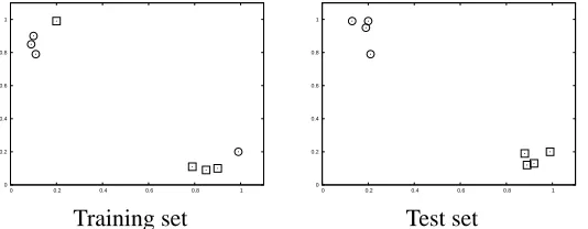
We can illustrate how the method works with a toy example. Consider the simple case of a two-dimensional space and the learning and testing sets shown in Figure 1. The figure shows how there are two points in the training set that are, with a high probability, mislabelled noisy data. Using these two data sets we run our algorithm and ADABOOSTwith an ensemble of 50 classifiers and a neural network, a C4.5 tree and a support vector machine as base classifiers. The results are shown in Table 1.

0 0.2 0.4 0.6 0.8 1

Training set Test set

Figure 1: Training and testing data for a two-dimensional problem of two classes with two likely mislabelled noisy instances

The example illustrates the differences of our method with boosting methods and how these differences may constitute an advantage. After the initial classifier is trained, ADABOOSTfocus its

effort on classifying the two misclassified instances correctly. The result is that the learning error drops eventually to 0, but the cost is overlearning the training data and poor generalisation. On the other hand, our method tries to classify the misclassified instances but without allowing the classifier to put too much effort on that task. The result is that the learning error is larger but the generalisation ability is better. This is, of course, a toy problem only intended to illustrate the underlying ideas of our method.

Base classifier Ensemble method

ADABOOST NLBP

Training Test Training Test Neural network 0.0000 0.5000 0.2500 0.0000 Support vector machine 0.0000 0.2500 0.2500 0.0000

C4.5 0.0000 0.2500 0.1250 0.1250

Table 1: Summary of training and test error results for the toy problem with an ensemble of 50 classifiers.

3. Related Work

(8)

and Duin, 2001). The random subspace method has been successfully applied to different problems (Munro et al., 2003; Hall et al., 2003).

Opitz (1999) developed accurate and diverse classifiers for an ensemble using ensemble feature selection. In contrast to classical feature selection algorithms, that are focused on finding the best feature subset for a given classifier, ensemble feature selection adds an additional objective of pro-moting disagreement among the individual classifiers. Different strategies have been proposed to ensemble feature selection, such as hill climbing (Kohavi, 1995; Cunningham and Carney, 2000), a genetic algorithm (Opitz, 1999), and the heuristic method Ensemble Forward and Backward Se-quential Selection (Aha and Bankert, 1995). A comparative study for medical diagnosis tasks is carried out in Tsymbal et al. (2003).

Utsugi (2001) proposed an ensemble of independent factor analysers (Anderson, 1984). This new statistical model assumes that each data point is generated by the sum of outputs of inde-pendently activated factor analysers. A maximum likelihood (ML) estimation algorithm for the parameters is derived using a Monte Carlo EM algorithm with a Gibbs sampler. The independent factor analysers developed into feature detectors that resemble complex cells in mammalian visual systems.

Yand et al. (2000) used mixtures of linear subspaces to create a classifier for face recognition. Rodr´ıguez et al. (2006) proposed a method based on applying PCA to subsets of inputs variables. The method obtained very good results on a large set of real-world problems.

4. Experiments

In order to test the performance of our method on solving classification tasks, we need to compare it with other widely used ensemble methods. In this section we try to make as fair a comparison as possible. So, we have chosen three different base classifiers: a neural network, a C4.5 tree (Quinlan, 1993), and a support vector machine (SVM) (Cristianini and Shawe-Taylor, 2000) . The first two have been widely used for ensemble construction in the literature. The last one has been shown recently to achieve good results as a member of an ensemble (Kim et al., 2002; Diao et al., 2002), although its stability might suggest that it is not a suitable base learner for constructing an ensemble. For the SVM we used a Gaussian kernel and parameters C=10.0 andγ=0.1. We used theLIBSVM

library (Chang and Lin, 2001). For the neural network we used a standard multilayer perceptron trained using a simple back-propagation algorithm (Rumelhart et al., 1986). The network has a hidden layer of 25 nodes and hyperbolic tangent transfer function for the hidden layer and logistic transfer function for the output layer. The network was trained for 100,000 iterations with a learning coefficientη=0.25 and a momentum coefficientα=0.1. For C4.5 we used the available code by the author of the algorithm. We must state that these parameters are rather standard and have not been selected in any way to improve the performance of any of the methods.2

For all three base classifiers we performed experiments using bagging, Arc-x4, ADABOOST, and MADABOOST(Domingo and Watanabe, 2000).

Before deciding upon bagging we tested its performance against wagging. Wagging is a variant of bagging (Breiman, 1996a) that requires a learning algorithm that can use training instances with different weights. Wagging assigns random weights to the instances of the training set instead of

(9)

resampling the training instances as in bagging. In our implementation the weights assigned to the instances follow a Poisson distribution (Webb, 2000). In a preliminary set of experiments we com-pared the performance of bagging and wagging, and found that bagging significantly outperformed wagging, so in all the experiments we have used bagging.

We use the Arc-x4 (Breiman, 1998) implementation in Bauer and Kohavi (1999). The factor (1+e(x)4₎ _{that weights each instance is rather heuristic, and the value of 4 for the exponent was} experimentally obtained as optimal. These type of methods were named by Breiman (1998) Arcing methods after “Adaptively resampling and combining”.

The ADABOOSTalgorithm is specifically designed for minimising the exponential loss func-tion:

m

∑

i=1

exp(₋yifλ(xi)),

where:

f_λ(xi) = n

∑

j=1

λjhj(xi).

One of the most interesting features of ADABOOSTis that the test error continues to improve, even when the learning error reaches 0 (Schapire et al., 1998). However, the marginal error reduction produced by each new classifier tends to decrease. On average, each new classifier has less impact on the test error than the previous members of the ensemble.

We use the ADABOOSTversion in Webb (2000). For ADABOOSTit is required that the weak learning algorithm, in our case each individual classifier, achieves an error strictly less than 0.5. This cannot be guaranteed; especially when dealing with difficult multiclass problems. In our ex-periments when this error is not achieved, we generate a bootstrap sample from the original set and continue the algorithm assigning to that classifier a zero weight (Bauer and Kohavi, 1999; Zhou et al., 2002).

For the three base learners we make a preliminary test to compare resampling and reweighting versions of the boosting algorithms. For neural networks we found that reweighting performed better than resampling; for C4.5 and SVM we found that resampling achieved better results. So, in the experiments reported here for the standard methods we use reweighting for neural networks, and resampling for C4.5 and SVMs.

For the case of a neural network as a base classifier we make some additional experiments to improve the quality of the comparison. Firstly, instead of using standard ADABOOST, we used ADABOOST.MH (Schapire and Singer, 1999, 2000). Moreover, we also used the algorithms GEN -TLEBOOST (Friedman et al., 2000) and LOGITBOOST (Friedman et al., 2000).3 Secondly, the hidden weights of the non-linear projection are also learned when using standard methods as an additional layer of the network, in order to avoid any spurious advantage for the proposed method derived from the use of the additional hidden layer represented by the non-linear projection.

All the ensembles are made up of 50 classifiers, regardless of the kind of base classifier. This number is fairly common in the literature. Although desirable, fixing the number of classifiers on

(10)

each ensemble taking into account either the problem or the type of base learner is computation-ally unfeasible. Moreover, it is known (Zenobi and Cunningham, 2001) that the diversity and the accuracy of the ensemble usually plateau at some size between 10 and 50 members. The standard ensembles are also made up of 50 networks. Furthermore, for ADABOOSTthe error bound of the training error is almost 0 after the addition of about 30 classifiers to the ensemble (Kuncheva, 2003), so 50 is a widely used ensemble size.

4.1 Experimental Setup

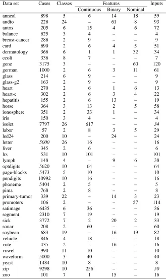
For testing the validity of the proposed method we have selected 44 data sets from the UCI Machine Learning Repository (Hettich et al., 1998). A summary of these data sets is shown in Table 2.

Three of the data sets were reduced to make them of a manageable size. For isolet and zip we performed a principal component analysis and retained the first 34 and 50 principal components respectively. For the letter data set we use a randomly selected subset of 5000 instances from the whole set of 20000 instances.

In order to avoid confusion we will use the term “learning error” for referring to the error of a classifier on the training set, and the term “test error” for the error of a classifier on the testing set. In the literature, the terms “generalisation error” and “prediction error” are also common for referring to the error on the test set. However, we believe that these two terms are more appropriate for the probability of misclassifying a new sample, thus the generalisation error is the expected test error.

The experiments were conducted following the 5x2 cross-validation set-up (Dietterich, 1998). We perform five replications of a two-fold cross-validation. In each replication the available data is partitioned into two random equal-sized sets. Each learning algorithm is trained on one set at a time and tested on the other set. The original test proposed by Dietterich suffers from low replicability, so to test the differences between two algorithms we use the 5x2cv F test (Alpaydin, 1999).

This test has the following formulation. We have five replications, i=1, . . . ,5, and two-folds, j=1,2, for each replication. p(_ij) is the difference between the error rates of the two classifiers on fold j of replication i. The average on replication i is ¯pi= (p_i(1)+p(_i2))/2, and the estimated variance is s2_i = ((p(_i1)₋¯pi)2+ ((p(_i2)−¯pi)2. Alpaydin (1999) proposed the test:

f =∑ 5

i=1∑2j=1

p(_ij)2

2∑5_i₌₁s2_i , (2)

that is approximately F distributed with 10 and 5 degrees of freedom. As a general rule we consider a confidence level of 90%. The same 5x2cv partitions were used for all the reported experiments.

In all tables the error measure is E = 1

n∑

n

i=1ei, where ei is 1 if instance i is misclassified and 0 otherwise. In the following sections we report all the experiments performed with the proposed method and all the data sets used for testing the method.

The source code, in C, used for the standard and proposed methods as well as the partitions of the data sets, are freely available upon request to the authors.

4.2 Experimental Results

In the first set of experiments we tested our method against the standard ensemble methods. For a neural network as base learner we used bagging, ADABOOST.MH, MADABOOST, LOGITBOOST,

(11)

Data set Cases Classes Features Inputs Continuous Binary Nominal

anneal 898 5 6 14 18 59

audio 226 24 – 61 8 93

autos 205 6 15 4 6 72

balance 625 3 4 – – 4

breast-cancer 286 2 9 – – 9

card 690 2 6 4 5 51

dermatology 366 6 1 1 32 34

ecoli 336 8 7 – – 7

gene 3175 3 – – 60 120

german 1000 2 6 3 11 61

glass 214 6 9 – – 9

glass-g2 163 2 9 – – 9

heart 270 2 6 1 6 13

heart-c 302 2 6 3 4 22

hepatitis 155 2 6 13 – 19

horse 364 3 13 2 5 58

ionosphere 351 2 33 1 – 34

iris 150 3 4 – – 4

isolet 7797 26 617 – – 34

labor 57 2 8 3 5 29

led24 200 10 – 24 – 24

letter 5000 26 16 – – 16

liver 345 2 6 – – 6

lrs 531 10 101 – – 101

lymph 148 4 – 9 6 38

optdigits 5620 10 64 – – 64

page-blocks 5473 5 10 – – 10

pendigits 10992 10 16 – – 16

phoneme 5404 2 5 – – 5

pima 768 2 8 – – 8

primary-tumor 339 22 – 14 3 23

promoters 106 2 – – 57 114

satimage 6435 6 36 – – 36

segment 2310 7 19 – – 19

sick 3772 7 2 20 2 33

sonar 208 2 60 – – 60

soybean 683 19 – 16 19 82

vehicle 846 4 18 – – 18

vote 435 2 – 16 – 16

vowel 990 11 10 – – 10

waveform 5000 3 40 – – 40

yeast 1484 10 8 – – 8

zip 9298 10 256 – – 50

zoo 101 7 1 15 – 16

(12)

results using C4.5 and SVM respectively. As explained, with these two base learners we have used bagging, ADABOOST, MADABOOST, and Arc-x4.

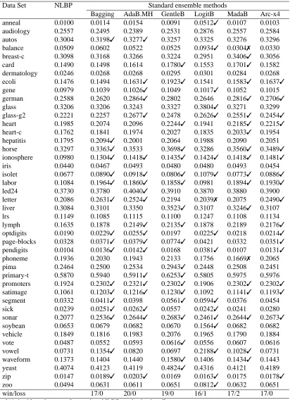
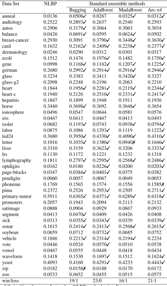
The results in Table 3 show that the proposed method is significantly better than the standard methods for 17 data sets when compared with bagging, 20 with ADABOOST.MH, 19 with GENTLE -BOOST, 16 with LOGITBOOST, 17 with MADABOOSTand Arc-x4. It is worse than LOGITBOOST

in 1 data set and worse than MADABOOSTin 2 data sets. The differences are not significant for the other data sets.

Table 4 shows the test error of NLBP and the four standard methods for C4.5 tree as base classifier. As a summary, NLBP is able to significantly improve bagging in 16 data sets, AdaBoost in 13, MadaBoost in 17 and Arc-x4 in 14. It is significantly worse in 3, 5, 3, and 3 data sets respectively. These results show a general advantage of our method. Nevertheless, the experiments using C4.5 as base learner show the worst performance of NLBP. We think the reason is the fact that C4.5 is a tree algorithm that best works with nominal and binary variables; the projection performed by NLBP transform all variables into continuous variables, and that may have a negative effect on C4.5 performance. However, even in this unfavourable scenario NLBP is able to outperform classical methods.

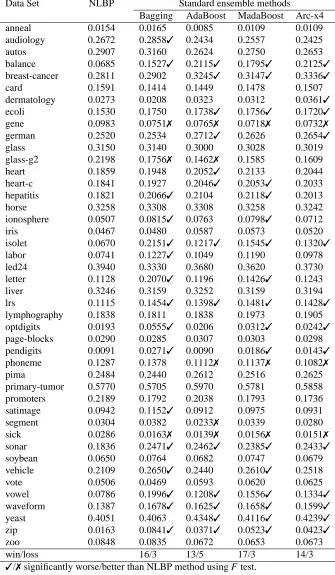
The results in Table 5 show that, for a SVM as base classifier, the proposed method is signifi-cantly better than bagging in 19 data sets, than ADABOOSTin 23 data sets, than MADABOOSTin

16 and than Arc-x4 in 21 data sets. NLBP is significantly worse than the standard methods only once for bagging, MADABOOST, and Arc-x4, and never for ADABOOST. In general terms, the performance of NLBP using a SVM as base classifier, is very good. We believe that the use of a SVM is able to obtain the best of NLBP as the non-linear projections obtained by NLBP are able to make the task of SVM easier.

As a summary, for all the three classifiers NLBP is able to obtain very good results, outper-forming both bagging and boosting methods. Of most interest is its performance in some of the most difficult problems, such as breast-cancer, hepatitis, horse, isolet, letter, liver, lymphography, primary-tumor, sonar, and vowel.

5. Analysis of the Proposed Method

In the previous section we have shown that the nonlinear projection approach is very competitive when compared with the standard methods of ensemble construction. In this section we present additional experiments that try to gain some insight into how it works.

In a first set of experiments we investigate if the good behaviour of NLBP is due to any side effect of the proposed algorithm or has its source in the idea of constructing nonlinear projections using only difficult instances. Then, we review theκ-error diagrams and show theκ-error diagrams of the standard and proposed methods. The behaviour of NLBP shown byκ-error diagrams suggests a further study on the sensitivity to noise of the method; that study is performed for all the data sets used in the previous experiments, and the three base classifiers.

5.1 Control Experiments

(13)

Data Set NLBP Standard ensemble methods

Bagging AdaB.MH GentleB LogitB MadaB Arc-x4 anneal 0.0100 0.0114 0.0154 0.0091 0.0512✓ 0.0107 0.0103 audiology 0.2557 0.2495 0.2389 0.2531 0.2876 0.2557 0.2584 autos 0.3004 0.3198✓ 0.3277✓ 0.3257 0.3325 0.3276 0.3296 balance 0.0509 0.0602 0.0522 0.0525 0.0934✓ 0.0304✗ 0.0330 breast-c 0.3098 0.3168 0.3266 0.3224 0.2951 0.3406✓ 0.3056 card 0.1490 0.1498 0.1614 0.1780✓ 0.1553 0.1701✓ 0.1582 dermatology 0.0246 0.0268 0.0268 0.0295 0.0301 0.0284 0.0268 ecoli 0.1476 0.1494 0.1631✓ 0.1923✓ 0.1541 0.1583✓ 0.1637✓

gene 0.0979 0.1039 0.1026✓ 0.1049 0.1017✓ 0.1052 0.1015 german 0.2588 0.2620 0.2864✓ 0.2802 0.2646 0.2816✓ 0.2706✓

glass 0.3206 0.3206 0.3243 0.3327 0.3804✓ 0.3271 0.3299 glass-g2 0.2221 0.2257 0.2677✓ 0.2478 0.2626✓ 0.2551✓ 0.2454✓

heart 0.1985 0.2074 0.2096 0.2244✓ 0.1941 0.2185✓ 0.2215✓

heart-c 0.1762 0.1841 0.1974 0.2027 0.1835 0.2033✓ 0.1954 hepatitis 0.1795 0.2094✓ 0.2001 0.2064 0.1988 0.2090 0.2051 horse 0.3297 0.3363✓ 0.3533 0.3698✓ 0.3286 0.3560✓ 0.3489✓

ionosphere 0.0980 0.1304✓ 0.1418✓ 0.1435✓ 0.1424✓ 0.1418✓ 0.1481✓

iris 0.0440 0.0467 0.0493 0.0480 0.0480 0.0493 0.0454

isolet 0.0677 0.0890✓ 0.0918✓ 0.0806✓ 0.1079✓ 0.0773✓ 0.0886✓

labor 0.1084 0.1964✓ 0.1860✓ 0.1858✓ 0.0981 0.1894✓ 0.1930✓

led24 0.3730 0.3780 0.4040✓ 0.3910 0.3870 0.3880 0.3900 letter 0.2086 0.2631✓ 0.2524✓ 0.2194 0.2039✗ 0.2075 0.2490✓

liver 0.3084 0.3101 0.3350 0.3523✓ 0.3107 0.3246✓ 0.3107

lrs 0.1149 0.1085 0.1115 0.1100 0.1247 0.1108 0.1134

lymph 0.1635 0.1878 0.2149✓ 0.2135✓ 0.1878 0.2189 0.2176✓

optdigits 0.0190 0.0229✓ 0.0255✓ 0.0197 0.0225✓ 0.0218 0.0214✓

page-blocks 0.0328 0.0371✓ 0.0379✓ 0.0774✓ 0.0421 0.0332 0.0351✓ pendigits 0.0104 0.0136✓ 0.0142✓ 0.0168 0.0381✓ 0.0107 0.0131✓

phoneme 0.1936 0.2030 0.1943 0.2133 0.1756 0.1669✗ 0.2065

pima 0.2464 0.2500 0.2534 0.2943✓ 0.2448 0.2508 0.2451

primary-t 0.5870 0.5940 0.5911✓ 0.6253✓ 0.5805 0.5975 0.5976 promoters 0.1924 0.2302✓ 0.2321✓ 0.2302✓ 0.1906 0.2302✓ 0.2302✓

satimage 0.1061 0.1203✓ 0.1216✓ 0.1230✓ 0.1092 0.1141✓ 0.1193✓

segment 0.0332 0.0411✓ 0.0398 0.0561✓ 0.0594✓ 0.0376 0.0454 sick 0.0239 0.0251✓ 0.0262✓ 0.0557 0.0242✓ 0.0241 0.0280 sonar 0.2077 0.2536✓ 0.2644✓ 0.2683✓ 0.2461✓ 0.2644✓ 0.2673✓

soybean 0.0653 0.0679 0.0682 0.0670 0.1564✓ 0.0682 0.0682 vehicle 0.1849 0.1816 0.1983 0.2076 0.1965 0.1790 0.1884

vote 0.0487 0.0552 0.0593 0.0616✓ 0.0556 0.0607 0.0616

vowel 0.0731 0.1354✓ 0.0820 0.0697 0.2188✓ 0.1028✓ 0.0731 waveform 0.1373 0.1404 0.1440 0.1580✓ 0.1406 0.1434✓ 0.1443 yeast 0.4074 0.4123 0.4119 0.4824✓ 0.4316 0.4121 0.4189 zip 0.0147 0.0189✓ 0.0203✓ 0.0169 0.0163✓ 0.0175 0.0178✓

zoo 0.0494 0.0631 0.0611 0.0651 0.0812✓ 0.0632 0.0651

win/loss 17/0 20/0 19/0 16/1 17/2 17/0

✓/✗significantly worse/better than NLBP method using F test.

(14)

Data Set NLBP Standard ensemble methods Bagging AdaBoost MadaBoost Arc-x4

anneal 0.0154 0.0165 0.0085 0.0109 0.0109

audiology 0.2672 0.2858✓ 0.2434 0.2557 0.2425

autos 0.2907 0.3160 0.2624 0.2750 0.2653

balance 0.0685 0.1527✓ 0.2115✓ 0.1795✓ 0.2125✓

breast-cancer 0.2811 0.2902 0.3245✓ 0.3147✓ 0.3336✓

card 0.1591 0.1414 0.1449 0.1478 0.1507

dermatology 0.0273 0.0208 0.0323 0.0312 0.0361✓

ecoli 0.1530 0.1750 0.1738✓ 0.1756✓ 0.1720✓

gene 0.0983 0.0751✗ 0.0765✗ 0.0718✗ 0.0732✗

german 0.2520 0.2534 0.2712✓ 0.2626 0.2654✓

glass 0.3150 0.3140 0.3000 0.3028 0.3019

glass-g2 0.2198 0.1756✗ 0.1462✗ 0.1585 0.1609

heart 0.1859 0.1948 0.2052✓ 0.2133 0.2044

heart-c 0.1841 0.1927 0.2046✓ 0.2053✓ 0.2033 hepatitis 0.1821 0.2066✓ 0.2104 0.2118✓ 0.2013

horse 0.3258 0.3308 0.3308 0.3258 0.3242

ionosphere 0.0507 0.0815✓ 0.0763 0.0798✓ 0.0712

iris 0.0467 0.0480 0.0587 0.0573 0.0520

isolet 0.0670 0.2151✓ 0.1217✓ 0.1545✓ 0.1320✓

labor 0.0741 0.1227✓ 0.1049 0.1190 0.0978

led24 0.3940 0.3330 0.3680 0.3620 0.3730

letter 0.1128 0.2070✓ 0.1196 0.1426✓ 0.1243

liver 0.3246 0.3159 0.3252 0.3159 0.3194

lrs 0.1115 0.1454✓ 0.1398✓ 0.1481✓ 0.1428✓

lymphography 0.1838 0.1811 0.1838 0.1973 0.1905 optdigits 0.0193 0.0555✓ 0.0206 0.0312✓ 0.0242✓

page-blocks 0.0290 0.0285 0.0307 0.0303 0.0298 pendigits 0.0091 0.0271✓ 0.0090 0.0186✓ 0.0143✓

phoneme 0.1287 0.1378 0.1112✗ 0.1137✗ 0.1082✗

pima 0.2484 0.2440 0.2612 0.2516 0.2625

primary-tumor 0.5770 0.5705 0.5970 0.5781 0.5858

promoters 0.2189 0.1792 0.2038 0.1793 0.1736

satimage 0.0942 0.1152✓ 0.0912 0.0975 0.0931

segment 0.0304 0.0382 0.0233✗ 0.0339 0.0280

sick 0.0286 0.0163✗ 0.0139✗ 0.0156✗ 0.0151✗

sonar 0.1836 0.2471✓ 0.2462✓ 0.2385✓ 0.2433✓

soybean 0.0650 0.0764 0.0682 0.0747 0.0679

vehicle 0.2109 0.2650✓ 0.2440 0.2610✓ 0.2518

vote 0.0506 0.0469 0.0593 0.0620 0.0625

vowel 0.0786 0.1996✓ 0.1208✓ 0.1556✓ 0.1334✓

waveform 0.1387 0.1678✓ 0.1625✓ 0.1658✓ 0.1599✓

yeast 0.4051 0.4063 0.4348✓ 0.4116✓ 0.4239✓

zip 0.0163 0.0841✓ 0.0371✓ 0.0523✓ 0.0423✓

zoo 0.0848 0.0835 0.0672 0.0653 0.0673

win/loss 16/3 13/5 17/3 14/3

(15)

Data Set NLBP Standard ensemble methods Bagging AdaBoost MadaBoost Arc-x4 anneal 0.0136 0.0508✓ 0.0267 0.0325✓ 0.0312✓

audiology 0.2522 0.2893✓ 0.2637 0.2540 0.2593

autos 0.2906 0.3179✓ 0.3064 0.3063 0.3034

balance 0.0426 0.0691✓ 0.0595 0.0624✓ 0.0502 breast-cancer 0.2930 0.3091 0.3790✓ 0.3448✓ 0.3630✓

card 0.1632 0.2162✓ 0.2409✓ 0.2238✓ 0.2377✓ dermatology 0.0246 0.0290 0.0312 0.0301 0.0317

ecoli 0.1512 0.1476 0.1976✓ 0.1482 0.1750✓

gene 0.0998 0.1168✓ 0.1162✓ 0.1207✓ 0.1225✓

german 0.2680 0.2992✓ 0.2914✓ 0.2916✓ 0.2946✓

glass 0.3234 0.3383 0.3411 0.3420✓ 0.3327

glass-g2 0.2098 0.2248 0.2196 0.2063 0.2210

heart 0.1844 0.1956✓ 0.2281✓ 0.2119✓ 0.2244✓

heart-c 0.1940 0.2126 0.2510✓ 0.2331✓ 0.2417✓

hepatitis 0.1847 0.1899 0.1948 0.1911 0.1936

horse 0.3440 0.3698✓ 0.3692 0.3648✓ 0.3654

ionosphere 0.0496 0.0547 0.0644 0.0581 0.0576

iris 0.0467 0.0413 0.0467 0.0413 0.0493

isolet 0.0682 0.1193✓ 0.0743 0.0938✓ 0.0794✓

labor 0.0875 0.1086 0.1293✓ 0.1119 0.1222✓

led24 0.3680 0.3950✓ 0.4330✓ 0.4090✓ 0.4310✓ letter 0.1016 0.1035✓ 0.1380✓ 0.0940✗ 0.1646✓

liver 0.3310 0.3159 0.3623✓ 0.3206 0.3333✓

lrs 0.1130 0.1172 0.1221 0.1232 0.1318

lymphography 0.1811 0.2797✓ 0.2595✓ 0.2568✓ 0.2486✓

optdigits 0.0162 0.0180 0.0226✓ 0.0200 0.0203✓

page-blocks 0.0347 0.0384✓ 0.0401✓ 0.0375 0.0382

pendigits 0.0060 0.0057 0.0067 0.0049 0.0053

phoneme 0.1769 0.1565 0.1574 0.1556 0.1585✗

pima 0.2372 0.2526 0.2953✓ 0.2505 0.2711✓

primary-tumor 0.5911 0.6365✓ 0.6371✓ 0.6289✓ 0.6318✓

promoters 0.2057 0.1943 0.2094 0.2113 0.2132

satimage 0.0888 0.0904 0.0929 0.0867 0.0933

segment 0.0413 0.0470✓ 0.0409 0.0426 0.0408

sick 0.0313 0.0355✓ 0.0343✓ 0.0339 0.0339✓

sonar 0.1615 0.2414✓ 0.2413✓ 0.2568✓ 0.2615✓

soybean 0.0659 0.0712 0.0732✓ 0.0685 0.0752

vehicle 0.1846 0.2213✓ 0.2314✓ 0.2194✓ 0.2234

vote 0.0446 0.0524 0.0570✓ 0.0510 0.0538

vowel 0.0467 0.0555 0.0448 0.0418 0.0434

waveform 0.1418 0.1530 0.1697✓ 0.1512 0.1624✓

yeast 0.4093 0.4160 0.4291✓ 0.4233 0.4443✓

zip 0.0182 0.0158✗ 0.0188 0.0170 0.0172

zoo 0.0533 0.0652 0.0455 0.0515 0.0575

win/loss 19/1 23/0 16/1 21/1

(16)

The first experiment tests if the performance of the method is due to the use of different pro-jections. It is known that the use of random subspaces is able to improve the performance of an ensemble (Ho, 1998), and it is possible that the use of different projections of the original data, no matter how they are obtained, could be the cause of the good performance of NLBP. So we have trained the classifiers that make up the ensemble using a different nonlinear random projection for each classifier. The random nonlinear projection is obtained using the same neural network used in NLBP, but with the weights randomly initialised in the interval[₋1,1]and no training.

The second experiment aims to establish if a similar performance can be obtained if we obtain different nonlinear projections using all the instances of the training set instead of only the misclas-sified instances. Thus, for this simulation, we apply Algorithm 1 but projection P(x)is constructed using the whole training set, S, instead of the subset of instances incorrectly classified by the pre-vious classifier, S0. The results of these two experiments for the three base classifiers are shown in Table 6.

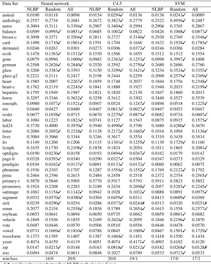
The table shows how NLBP is performing significantly better than the two control algorithms for many problems. This experiment supports the approach of the proposed algorithm, ruling out as a cause of its good performance the use of an additional layer of learning. For a neural network NLBP is significantly better than a random projection in 16 data sets, and better than the projection using all the instances in 20 data sets. Similar results are obtained for a C4.5 tree and a SVM.

5.2 κ- Error Diagrams

One way of understanding the behaviour of ensemble methods is by means of aκ-error diagram (Margineantu and Dietterich, 1997; Dietterich, 2000a). These diagrams represent a point for each pair of classifiers. The x coordinate is a measure of the diversity of the two classifiers known asκ measure, the y coordinate is the average error of the two classifiers on the test data. The two values are conflicting, as it is obvious that we cannot have both perfect and independent classifiers. The κ-error diagram is the scatter plot of the points corresponding to all pairs of classifiers.

The κmeasure is defined as follows: let us consider a problem with K classes, and let C be a K_×K matrix such that Ci j contains the number of instances assigned to class i by the first classifier and to class j by the second classifier. Let us define:

Θ1=∑ K

i=1Cii

n ,

and

Θ2= K

∑

i=1

K

∑

j=1

Ci j n ×

K

∑

j=1

Cji n

! ,

where n is the number of instances. Then, theκstatistic is defined:

κ=Θ1−Θ2 1₋Θ2 .

(17)

Data Set Neural network C4.5 SVM

NLBP Random All NLBP Random All NLBP Random All

anneal 0.0100 0.0118 0.0096 0.0154 0.0294✓ 0.0136 0.0136 0.0243✓ 0.0089

audiology 0.2557 0.2734 0.2681 0.2672 0.3823✓ 0.2779 0.2522 0.4956✓ 0.2487

autos 0.3004 0.3111 0.3394✓ 0.2907 0.3404✓ 0.2994 0.2906 0.3765 0.2867

balance 0.0509 0.0995✓ 0.0851✓ 0.0685 0.1002✓ 0.0822 0.0426 0.1008✓ 0.0877✓

breast-c 0.3098 0.3371 0.3504✓ 0.2811 0.2727 0.3140✓ 0.2930 0.2769 0.3546✓

card 0.1490 0.1710✓ 0.1861✓ 0.1591 0.1704 0.1646 0.1632 0.1928✓ 0.1785✓

dermatol. 0.0246 0.0263 0.0301 0.0273 0.0306 0.0372✓ 0.0246 0.0306 0.0284

ecoli 0.1476 0.1363✓ 0.1512✓ 0.1530 0.1506 0.1655 0.1512 0.1512 0.1554

gene 0.0979 0.0996 0.1009✓ 0.0983 0.2363✓ 0.1253✓ 0.0998 0.3997✓ 0.1008

german 0.2588 0.2626✓ 0.2840✓ 0.2520 0.2592 0.2750✓ 0.2680 0.2686 0.2760

glass 0.3206 0.3383✓ 0.3393 0.3150 0.3299✓ 0.3421✓ 0.3234 0.3524✓ 0.3355✓

glass-g2 0.2221 0.2111 0.2417 0.2198 0.2444 0.2259 0.2098 0.2579✓ 0.2369✓

heart 0.1985 0.2007 0.2267✓ 0.1859 0.1748 0.2037 0.1844 0.1756 0.2348✓

heart-c 0.1762 0.2119 0.2245✓ 0.1841 0.1888 0.1927 0.1940 0.2033 0.2199✓

hepatitis 0.1795 0.1949 0.1987 0.1821 0.1820 0.2130 0.1847 0.1860 0.2013

horse 0.3297 0.3346 0.3632✓ 0.3258 0.3412 0.3302 0.3440 0.3527 0.3539

ionosph. 0.0980 0.1077✓ 0.1521✓ 0.0507 0.0524 0.1247✓ 0.0496 0.0518 0.1225✓

iris 0.0440 0.0427 0.0480 0.0467 0.0613✓ 0.0627✓ 0.0467 0.0453 0.0467

isolet 0.0677 0.1038✓ 0.0715 0.0670 0.2279✓ 0.0875✓ 0.0682 0.0734 0.0607✓

labor 0.1084 0.1223 0.1823✓ 0.0741 0.1127 0.1543 0.0875 0.0915 0.1575✓

led24 0.3730 0.4000 0.3970✓ 0.3940 0.4990✓ 0.3790 0.3680 0.4280✓ 0.3670

letter 0.2086 0.2692✓ 0.2328✓ 0.1128 0.2172✓ 0.1665✓ 0.1016 0.1094 0.1136✓

liver 0.3084 0.3066 0.3344 0.3246 0.3617 0.3554 0.3310 0.3438 0.3414

lrs 0.1149 0.1206 0.1206 0.1115 0.1341✓ 0.1255✓ 0.1130 0.1729✓ 0.1160

lymph. 0.1635 0.1730 0.2108✓ 0.1838 0.1824 0.2054 0.1811 0.1865 0.2081✓

optdigits 0.0190 0.0230✓ 0.0158 0.0193 0.0494✓ 0.0267✓ 0.0162 0.0179 0.0142

page-b 0.0328 0.0393✓ 0.0340 0.0290 0.0327✓ 0.0304 0.0347 0.0373 0.0329

pendigits 0.0104 0.0162✓ 0.0137✓ 0.0091 0.0133✓ 0.0132✓ 0.0060 0.0062 0.0075

phoneme 0.1936 0.2103 0.1707 0.1287 0.1554✓ 0.1552✓ 0.1769 0.2122✓ 0.1702

pima 0.2464 0.2396 0.2615 0.2484 0.2458 0.2518 0.2372 0.2354 0.2565✓

primary-t 0.5870 0.5846 0.5905 0.5770 0.5917 0.5793 0.5911 0.5823 0.5852

promoters 0.1924 0.2208 0.2283 0.2189 0.2434 0.2698✓ 0.2057 0.5283✓ 0.2245✓

satimage 0.1061 0.1154✓ 0.1142✓ 0.0942 0.1028 0.1032✓ 0.0888 0.0891 0.0975✓

segment 0.0332 0.0570✓ 0.0380✓ 0.0304 0.0459✓ 0.0311 0.0413 0.0609✓ 0.0369

sick 0.0239 0.0290✓ 0.0254 0.0286 0.0373✓ 0.0244✗ 0.0313 0.0320 0.0251✗

sonar 0.2077 0.2154 0.2558✓ 0.1836 0.1789 0.2654✓ 0.1615 0.1558 0.2577✓

soybean 0.0653 0.0641 0.0694 0.0650 0.0735 0.0662 0.0659 0.0861✓ 0.0682

vehicle 0.1849 0.1936 0.1835 0.2109 0.2624✓ 0.2059 0.1846 0.2196✓ 0.1870

vote 0.0487 0.0446 0.0570 0.0506 0.0510 0.0556 0.0446 0.0478 0.0570

vowel 0.0731 0.1669✓ 0.1810✓ 0.0786 0.0845 0.1069✓ 0.0467 0.1501✓ 0.1729✓

waveform 0.1373 0.1395 0.1407 0.1387 0.1604✓ 0.1451 0.1418 0.1550 0.1434

yeast 0.4074 0.4159 0.4119 0.4051 0.4074 0.4171✓ 0.4093 0.4102 0.4120

zip 0.0147 0.0215✓ 0.0148 0.0163 0.0818✓ 0.0212✓ 0.0182 0.0268✓ 0.0128✗

zoo 0.0494 0.0474 0.0611 0.0848 0.1027 0.0789 0.0533 0.0713✓ 0.0533

win/loss 16/0 20/0 20/0 19/1 17/0 17/2

(18)

Figures 2, 3, and 4 show κ-error diagrams of the first partition for several data sets with four standard methods and NLBP, and neural networks, C4.5, and SVMs as base classifiers, respectively. These diagrams are fairly representative of the diagrams of all the data sets.

For all the three base classifiers we verify the usual behaviour of bagging and boosting methods. Bagging provides diversity, but to a lesser degree than boosting. On the other hand, boosting’s improvement of diversity has the side effect of deteriorating accuracy. NLBP behaviour is midway between these two methods. It is able to improve diversity, but to a lesser degree than boosting, without damaging accuracy as much as boosting. This behaviour suggests that the performance of NLBP in noisy problems can be better than the performance of boosting methods. The next section is devoted to studying the sensitivity to noise of NLBP, and tests that hypothesis.

5.3 Effect of Noise

Several researchers have reported that boosting methods, among them ADABOOST, degrade their

performance in the presence of noise. Dietterich (2000a) tested this effect introducing artificial noise in the class labels of different data sets and confirmed this behaviour. In this section we study the sensitivity of our method to noise.

To add noise to the class labels we follow the method of Dietterich (2000a). To add classification noise at a rate r, we chose a fraction r of the instances and changed their class labels to be incorrect choosing uniformly from the set of incorrect labels. We chose all the data sets and three rates of noise, 5%, 10%, and 20%. With this three levels of noise we have performed the experiments using the 5x2cv setup and NLBP, bagging and ADABOOSTensemble methods and compared the results as the level of noise increases.

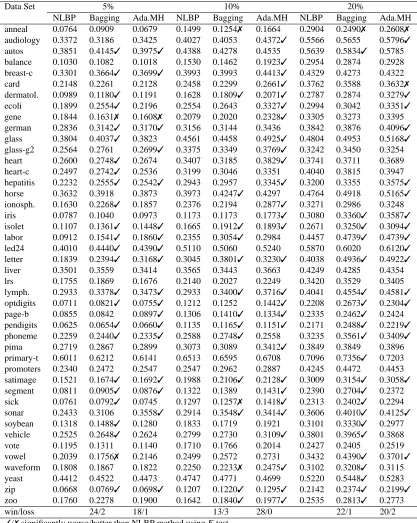
For the noise study we have used bagging and ADABOOSTas the representative of the boosting methods (for neural networks the used method is ADABOOST.MH as in the previous experiments). Tables 7, 8, and 9 show the comparison of the three methods at noise levels 5%, 10%, and 20%, for a neural network, a C4.5 tree and a SVM respectively. First of all, we can corroborate that tables confirm that bagging is less affected by noise than boosting, as has been shown in several papers, for example, (Dietterich, 2000a).

Table 7 shows the results for a neural network. For a noise level of 5% the results are not much different from the results without noise for all the three methods. Bagging performs slightly worse and ADABOOST.MH slightly better. It seems that for this low noise level the algorithms perform as in the case without noise. For 10% of noise the performance of bagging improves, achieving a win/loss record of 13/3 with NLBP, better than the record without noise, 17/0. On the other hand, the performance of ADABOOST.MH drops to a win/loss record of 28/0 with NLBP. Here the sensibility to noise of ADABOOST.MH is clearly evident.

(19)

NLBP ADABOOST.MH Arc-x4 Bagging MADABOOST

card

0 0.5 1

0 0.5 1 0 0.5 1

0 0.5 1

ecoli

0 0.5 1

0 0.5 1 0 0.5 1

0 0.5 1

german

0 0.5 1

0 0.5 1 0 0.5 1

0 0.5 1

heart

0 0.5 1

0 0.5 1 0 0.5 1

0 0.5 1

li v er 0 0.5 1

0 0.5 1 0 0.5 1

0 0.5 1

pima

0 0.5 1

0 0.5 1 0 0.5 1

0 0.5 1

v

ehicle

0 0.5 1

0 0.5 1 0 0.5 1

0 0.5 1

v o wel 0 0.5 1

0 0.5 1 0 0.5 1

0 0.5 1

yeast

0 0.5 1

0 0.5 1 0 0.5 1

0 0.5 1

(20)

NLBP ADABOOST Arc-x4 Bagging MADABOOST

audio

0 0.5 1

0 0.5 1 0 0.5 1

0 0.5 1

card

0 0.5 1

0 0.5 1 0 0.5 1

0 0.5 1

gene

0 0.5 1

0 0.5 1 0 0.5 1

0 0.5 1

ionosphere 0 0.5 1

0 0.5 1 0 0.5 1

0 0.5 1

li v er 0 0.5 1

0 0.5 1 0 0.5 1

0 0.5 1

lymph

0 0.5 1

0 0.5 1 0 0.5 1

0 0.5 1

pima

0 0.5 1

0 0.5 1 0 0.5 1

0 0.5 1

promoters 0 0.5 1

0 0.5 1 0 0.5 1

0 0.5 1

v o wel 0 0.5 1

0 0.5 1 0 0.5 1

0 0.5 1

(21)

NLBP ADABOOST Arc-x4 Bagging MADABOOST

breast-cancer 0 0.5 1

0 0.5 1 0 0.5 1

0 0.5 1

ecoli

0 0.5 1

0 0.5 1 0 0.5 1

0 0.5 1

glass

0 0.5 1

0 0.5 1 0 0.5 1

0 0.5 1

heart-c

0 0.5 1

0 0.5 1 0 0.5 1

0 0.5 1

li v er 0 0.5 1

0 0.5 1 0 0.5 1

0 0.5 1

lymph

0 0.5 1

0 0.5 1 0 0.5 1

0 0.5 1

pima

0 0.5 1

0 0.5 1 0 0.5 1

0 0.5 1

sonar

0 0.5 1

0 0.5 1 0 0.5 1

0 0.5 1

yeast

0 0.5 1

0 0.5 1 0 0.5 1

0 0.5 1

(22)

Using C4.5 as base learner, Table 8, the results are much the same. For a noise level of 5% the performance of the three algorithms is similar to the original one. When the noise level increases to 10% the performance of ADABOOSTdegrades from a win/loss record of 13/5 (with no artificial noise) to a record of 19/2. Bagging slightly worsens compared with NLBP, from a record of 16/3 to 20/6. When the noise level is 20% the effect is more marked for both algorithms, with a record of 18/3 for bagging and 25/1 for ADABOOST.

Table 9 shows a similar behaviour for the three algorithms when using a SVM but with some differences. The performance of ADABOOSTdramatically decreases with noise as in the previous cases. For a SVM the negative effect of noise on ADABOOSTis even more marked. But the case of

bagging is slightly different from the two previous classifiers. With a SVM bagging is less affected by noise, even improving its compared performance with NLBP; for a noise level of 20% bagging is worse than NLBP in only 11 data sets.

In summary, NLBP has the very desirable property of behaving, at least, as robustly as bagging in the presence of noise. This is probably due to the fact that NLBP does not put so much emphasis on incorrectly classified instances as boosting does. However, NLBP does use the incorrectly clas-sified instances in determining the nonlinear representation of the input data which provides it with a performance enhancement over bagging.

5.4 Effect of Ensemble Size

As we have stated, most previous work agrees that boosting methods are fairly resistant to over-fitting. Additionally, there is also a general agreement that the most important gain of boosting methods is given by the first few classifiers. These two arguments together support the use of an ensemble of fixed size of 50 base classifiers as reasonable, and that it is not likely that the size of the ensemble might contaminate the experimental results. Nevertheless, it is possible that for some of the problems the ensemble may be either overfitting or underfitting the data. So, we have performed an additional experiment where the size of the ensemble is obtained by a cross-validation strategy. The experiment is carried out using ADABOOSTand the proposed NLBP method.

The method for selecting the number of classifiers for each problem is the cross-validation strat-egy presented in Zhang and Yu (2005). For each partition of each problem we perform a 5-fold cross-validation to obtain the optimal size of the ensemble within the range of[10,100]classifiers. That is, we divide the training set into five partitions and train the ensemble with four partitions and test the error with the remaining one. This is repeated for each one of the five partitions, and the en-semble size is obtained as the average size of the 5 runs. Then, the algorithm is run with this optimal size of the ensemble and using the whole training set. As the size of the ensemble is estimated for each partition, overfitting or underfitting is less likely to happen. Table 10 shows the results using the three base classifiers of the previous experiments. The parameters of the experiments are the same as the previous runs.

The first noticeable result shown in the table is that the errors of the algorithms using this method are similar to the errors for ensembles of 50 classifiers. These results support the general belief that boosting is quite resistant to overfitting. The results also show that NLBP is also hardly affected by overfitting. The differences among NLBP and ADABOOSTare similar to the obtained using 50

(23)

Data Set 5% 10% 20%

NLBP Bagging Ada.MH NLBP Bagging Ada.MH NLBP Bagging Ada.MH

anneal 0.0764 0.0909 0.0679 0.1499 0.1254✗ 0.1664 0.2904 0.2490✗ 0.2608✗

audiology 0.3372 0.3186 0.3425 0.4027 0.4053 0.4372✓ 0.5566 0.5655 0.5796✓

autos 0.3851 0.4145✓ 0.3975✓ 0.4388 0.4278 0.4535 0.5639 0.5834✓ 0.5785

balance 0.1030 0.1082 0.1018 0.1530 0.1462 0.1923✓ 0.2954 0.2874 0.2928

breast-c 0.3301 0.3664✓ 0.3699✓ 0.3993 0.3993 0.4413✓ 0.4329 0.4273 0.4322

card 0.2148 0.2261 0.2128 0.2458 0.2299 0.2661✓ 0.3762 0.3588 0.3632✗

dermatol. 0.0989 0.1180✓ 0.1191 0.1628 0.1809✓ 0.2071✓ 0.2787 0.2874 0.3279✓

ecoli 0.1899 0.2554✓ 0.2196 0.2554 0.2643 0.3327✓ 0.2994 0.3042 0.3351✓

gene 0.1844 0.1631✗ 0.1608✗ 0.2079 0.2020 0.2328✓ 0.3305 0.3273 0.3395

german 0.2836 0.3142✓ 0.3170✓ 0.3156 0.3144 0.3436 0.3842 0.3876 0.4096✓

glass 0.3804 0.4037✓ 0.3823 0.4561 0.4458 0.4925✓ 0.4804 0.4953 0.5168✓

glass-g2 0.2564 0.2761 0.2699✓ 0.3375 0.3349 0.3769✓ 0.3242 0.3450 0.3254

heart 0.2600 0.2748✓ 0.2674 0.3407 0.3185 0.3829✓ 0.3741 0.3711 0.3689

heart-c 0.2497 0.2742✓ 0.2536 0.3199 0.3046 0.3351 0.4040 0.3815 0.3947

hepatitis 0.2232 0.2555✓ 0.2542✓ 0.2943 0.2957 0.3345✓ 0.3200 0.3355 0.3575✓

horse 0.3632 0.3918 0.3873 0.3973 0.4247✓ 0.4297 0.4764 0.4918 0.5165✓

ionosph. 0.1630 0.2268✓ 0.1857 0.2376 0.2194 0.2877✓ 0.3271 0.2986 0.3248

iris 0.0787 0.1040 0.0973 0.1173 0.1173 0.1773✓ 0.3080 0.3360✓ 0.3587✓

isolet 0.1107 0.1361✓ 0.1448✓ 0.1665 0.1912✓ 0.1893✓ 0.2671 0.3250✓ 0.3094✓

labor 0.0912 0.1541✓ 0.1860✓ 0.2355 0.3054✓ 0.2984 0.4457 0.4739✓ 0.4739✓

led24 0.4010 0.4440✓ 0.4390✓ 0.5110 0.5060 0.5240 0.5870 0.6020 0.6120✓

letter 0.1839 0.2394✓ 0.3168✓ 0.3045 0.3801✓ 0.3230✓ 0.4038 0.4936✓ 0.4922✓

liver 0.3501 0.3559 0.3414 0.3565 0.3443 0.3663 0.4249 0.4285 0.4354

lrs 0.1755 0.1869 0.1676 0.2140 0.2027 0.2249 0.3420 0.3529 0.3405

lymph. 0.2933 0.3378✓ 0.3473✓ 0.2933 0.3400✓ 0.3716✓ 0.4041 0.4554✓ 0.4581✓

optdigits 0.0711 0.0821✓ 0.0755✓ 0.1212 0.1252 0.1442✓ 0.2208 0.2673✓ 0.2304✓

page-b 0.0855 0.0842 0.0897✓ 0.1306 0.1410✓ 0.1334✓ 0.2335 0.2462✓ 0.2424

pendigits 0.0625 0.0654✓ 0.0660✓ 0.1135 0.1165✓ 0.1151✓ 0.2171 0.2488✓ 0.2219✓

phoneme 0.2259 0.2440✓ 0.2335✓ 0.2588 0.2748✓ 0.2558 0.3235 0.3561✓ 0.3409✓

pima 0.2719 0.2867 0.2899 0.3073 0.3089 0.3412✓ 0.3849 0.3849 0.3896

primary-t 0.6011 0.6212 0.6141 0.6513 0.6595 0.6708 0.7096 0.7356✓ 0.7203

promoters 0.2340 0.2472 0.2547 0.2547 0.2962 0.2887 0.4245 0.4472 0.4453

satimage 0.1521 0.1674✓ 0.1692✓ 0.1988 0.2106✓ 0.2128✓ 0.3009 0.3154✓ 0.3058✓

segment 0.0811 0.0905✓ 0.0876✓ 0.1322 0.1389 0.1431✓ 0.2390 0.2704✓ 0.2372

sick 0.0761 0.0792✓ 0.0745 0.1297 0.1257✗ 0.1418✓ 0.2313 0.2402✓ 0.2294

sonar 0.2433 0.3106 0.3558✓ 0.2914 0.3548✓ 0.3414✓ 0.3606 0.4010✓ 0.4125✓

soybean 0.1318 0.1488✓ 0.1280 0.1833 0.1719 0.1921 0.3101 0.3330✓ 0.2977

vehicle 0.2525 0.2648✓ 0.2624 0.2799 0.2730 0.3109✓ 0.3801 0.3965✓ 0.3868

vote 0.1195 0.1311 0.1140 0.1710 0.1766 0.2014 0.2427 0.2405 0.2519

vowel 0.2039 0.1756✗ 0.2146 0.2499 0.2572 0.2731 0.3432 0.4390✓ 0.3701✓

waveform 0.1808 0.1867 0.1822 0.2250 0.2233✗ 0.2475✓ 0.3102 0.3208✓ 0.3115

yeast 0.4412 0.4522 0.4473 0.4747 0.4771 0.4699 0.5220 0.5448✓ 0.5283

zip 0.0668 0.0769✓ 0.0698✓ 0.1207 0.1220✓ 0.1295✓ 0.2142 0.2374✓ 0.2199✓

zoo 0.1760 0.2278 0.1900 0.1642 0.1840✓ 0.1977✓ 0.2535 0.2813✓ 0.2773

win/loss 24/2 18/1 13/3 28/0 22/1 20/2

(24)

Data Set 5% 10% 20%

NLBP Bagging AdaB NLBP Bagging AdaB NLBP Bagging AdaB

anneal 0.0722 0.0973✓ 0.0922 0.1399 0.1817✓ 0.1757✓ 0.2702 0.3156✓ 0.3200✓

audiology 0.3460 0.3027 0.3106 0.3717 0.3566✗ 0.3593✗ 0.5620 0.5195✗ 0.5204✗

autos 0.3871 0.3413✗ 0.3725 0.4214 0.3853 0.3911 0.5288 0.5307 0.5367

balance 0.1296 0.3567✓ 0.2586✓ 0.1718 0.2883✓ 0.3082✓ 0.3139 0.4198✓ 0.4292✓

breast-c 0.3014 0.3007 0.3469 0.3455 0.3881✓ 0.4028✓ 0.3993 0.4182 0.4392✓

card 0.2029 0.1893 0.1942 0.2371 0.2313 0.2386 0.3495 0.3551 0.3649

dermatol. 0.0891 0.1060 0.0951 0.1563 0.1836✓ 0.1776✓ 0.2311 0.2475✓ 0.2503✓

ecoli 0.1976 0.2125✓ 0.2167 0.2494 0.2923✓ 0.2976✓ 0.2881 0.3298✓ 0.3500✓

gene 0.1542 0.1312✗ 0.1451 0.2023 0.1746✗ 0.1996 0.3242 0.2905✗ 0.3227

german 0.2916 0.2912 0.2974 0.3126 0.3320 0.3292 0.3796 0.3904 0.4086✓

glass 0.3841 0.3710 0.3729 0.4393 0.4047 0.4112 0.4738 0.4467 0.4645

glass-g2 0.2627 0.2418 0.2455 0.3350 0.2982 0.3153 0.3316 0.3168 0.3608

heart 0.2445 0.2607 0.2652 0.2941 0.3200 0.3437✓ 0.3378 0.3667 0.3830

heart-c 0.2311 0.2583✓ 0.2583✓ 0.2921 0.3066 0.3175✓ 0.3536 0.3960✓ 0.3987

hepatitis 0.2259 0.2296 0.2308 0.3021 0.2763✗ 0.2983✗ 0.2956 0.3047 0.3073

horse 0.3637 0.3522 0.3610 0.3923 0.3995 0.4099 0.4698 0.5066 0.5094✓

ionosph. 0.1459 0.1305 0.1464 0.1715 0.1881 0.1898 0.2706 0.2957 0.3031

iris 0.1027 0.1094 0.1027 0.1147 0.1707✓ 0.1720✓ 0.3173 0.3560✓ 0.3667✓

isolet 0.1152 0.2102✓ 0.1706✓ 0.1646 0.2489✓ 0.2189✓ 0.2635 0.3215✓ 0.3202✓

labor 0.1050 0.1085 0.1117 0.1863 0.1898 0.1792 0.3576 0.3825 0.3785

led24 0.4350 0.4120 0.4150 0.5270 0.4850 0.4970 0.5860 0.5480 0.5610

letter 0.1645 0.2106✓ 0.1893✓ 0.2137 0.2499✓ 0.2502✓ 0.3222 0.3709✓ 0.3782✓

liver 0.3768 0.3698 0.3565 0.3843 0.3663 0.3722 0.4493 0.4337 0.4482

lrs 0.1737 0.1936 0.1959✓ 0.2098 0.2219✓ 0.2174 0.3081 0.3326 0.3296

lymph. 0.2838 0.2838 0.2865 0.2906 0.3203 0.3230 0.3460 0.3851✓ 0.4081✓

optdigits 0.0700 0.0873✓ 0.0716 0.1207 0.1352✓ 0.1244 0.2223 0.2310✓ 0.2311✓

page-b 0.0794 0.0842✓ 0.0849✓ 0.1311 0.1400✓ 0.1389✓ 0.2312 0.2528✓ 0.2526✓

pendigits 0.0588 0.0680✓ 0.0614✓ 0.1080 0.1167✓ 0.1154✓ 0.2118 0.2247✓ 0.2245✓

phoneme 0.2110 0.1814 0.1716✗ 0.2563 0.2075✗ 0.2245 0.3247 0.3007✗ 0.3340

pima 0.2794 0.2857 0.2927 0.3169 0.3372 0.3331 0.3818 0.3974 0.4083✓

primary-t 0.5941 0.6135 0.6064 0.6430 0.6519 0.6814 0.6902 0.7126 0.7338✓

promoters 0.2358 0.2113 0.1887 0.2793 0.2264✗ 0.2547 0.4151 0.4170 0.4170

satimage 0.1385 0.1476✓ 0.1391 0.1833 0.1903✓ 0.1860✓ 0.2849 0.2853 0.2864

segment 0.0820 0.0827 0.0887✓ 0.1345 0.1448✓ 0.1483✓ 0.2446 0.2549 0.2613✓

sick 0.0871 0.0674✗ 0.0720✗ 0.1422 0.1290✗ 0.1442 0.2387 0.2521 0.2818✓

sonar 0.3039 0.2692 0.2769 0.3433 0.3308 0.3260 0.3442 0.3577 0.3837✓

soybean 0.1256 0.1616✓ 0.1529 0.1754 0.2234✓ 0.2100✓ 0.3051 0.3640✓ 0.3643✓

vehicle 0.2645 0.3024✓ 0.3111✓ 0.2976 0.3303✓ 0.3343✓ 0.4047 0.4388✓ 0.4310

vote 0.1154 0.1310 0.1297 0.1697 0.1904✓ 0.1959 0.2349 0.2630✓ 0.2731✓

vowel 0.1758 0.2085✓ 0.1957 0.2244 0.2628✓ 0.2554✓ 0.3321 0.3667✓ 0.3675✓

waveform 0.1821 0.2028✓ 0.2045✓ 0.2260 0.2432✓ 0.2487✓ 0.3142 0.3292 0.3364✓

yeast 0.4464 0.4580 0.4625✓ 0.4791 0.4945 0.4988 0.5367 0.5566✓ 0.5616✓

zip 0.0676 0.1107✓ 0.0874✓ 0.1201 0.1596✓ 0.1404✓ 0.2171 0.2390✓ 0.2383✓

zoo 0.1859 0.1799 0.2016 0.1841 0.1702 0.2038 0.2653 0.2594 0.2713

win/loss 15/3 12/2 20/6 19/2 18/3 25/1

(25)

Data Set 5% 10% 20%

NLBP Bagging AdaB NLBP Bagging AdaB NLBP Bagging AdaB

anneal 0.0757 0.1031✓ 0.1238✓ 0.1635 0.1682 0.2007✓ 0.3114 0.3027 0.3575✓

audiology 0.3469 0.3522 0.5611✓ 0.5620 0.4265✗ 0.4310✗ 0.6691 0.5761✗ 0.6035

autos 0.3881 0.3803 0.4671✓ 0.4643 0.4262 0.4418 0.5630 0.5463 0.5727

balance 0.1088 0.1264✓ 0.1760✓ 0.1626 0.1680 0.2003✓ 0.3094 0.3146 0.3421✓

breast-c 0.3182 0.3602✓ 0.4147✓ 0.3727 0.3930✓ 0.4301✓ 0.4154 0.4273 0.4594

card 0.2180 0.2658✓ 0.3049✓ 0.2826 0.2907 0.3249✓ 0.3875 0.3899 0.4160✓

dermatol. 0.1011 0.0896 0.1465✓ 0.1667 0.1656 0.2197✓ 0.2574 0.2579 0.3344✓

ecoli 0.1887 0.1839 0.2732✓ 0.2476 0.2488 0.3226✓ 0.2792 0.2798 0.3607✓

gene 0.1857 0.2050✓ 0.3099✓ 0.3482 0.2584 0.2869 0.3244 0.3707✓ 0.4001✓

german 0.3000 0.3150✓ 0.3150 0.3242 0.3310✓ 0.3394 0.3780 0.3800 0.3872

glass 0.3729 0.3841 0.4028 0.4327 0.4439 0.4823 0.4682 0.4907✓ 0.5252✓

glass-g2 0.2651 0.2652 0.2565 0.3276 0.3117✗ 0.3351 0.3192 0.3266 0.3425

heart 0.2333 0.2459 0.2852✓ 0.2830 0.3104✓ 0.3622✓ 0.3452 0.3763 0.3978✓

heart-c 0.2537 0.2596✓ 0.3192✓ 0.2914 0.3033 0.3576✓ 0.3715 0.3854 0.4245✓

hepatitis 0.2194 0.2299 0.2284 0.2866 0.2724 0.2879 0.2866 0.3111 0.3278

horse 0.3709 0.3989✓ 0.3989 0.4116 0.4220 0.4160 0.4846 0.4808 0.4879

ionosph. 0.1026 0.1066 0.1391✓ 0.1738 0.1721 0.2165✓ 0.2684 0.2712 0.3253✓

iris 0.0746 0.0760 0.1013 0.1027 0.1040 0.1414 0.3133 0.3013 0.3347

isolet 0.1101 0.1675✓ 0.1721✓ 0.1839 0.2144✓ 0.2286✓ 0.2893 0.3163✓ 0.3375✓

labor 0.0979 0.0915 0.1224 0.2005 0.2246 0.2491✓ 0.3510 0.3791 0.4179✓

led24 0.4040 0.4270 0.4730✓ 0.5270 0.5120 0.5360 0.5910 0.5740 0.6010

letter 0.1859 0.1716✗ 0.2432 0.2399 0.2286 0.2683✓ 0.3507 0.3647✓ 0.4168✓

liver 0.3519 0.3478 0.3762 0.3629 0.3588 0.3890 0.4209 0.4238 0.4592✓

lrs 0.1752 0.1789 0.2079✓ 0.2554 0.2268 0.2931 0.3627 0.3439 0.4620

lymph. 0.2838 0.3392✓ 0.3176 0.2906 0.4054✓ 0.3325 0.3730 0.4297✓ 0.4216

optdigits 0.0730 0.0975✓ 0.1339✓ 0.1276 0.1736✓ 0.2368✓ 0.2453 0.2857✓ 0.3411✓

page-b 0.0865 0.0894 0.0919 0.1346 0.1495✓ 0.1388 0.2381 0.2598✓ 0.2396

pendigits 0.0605 0.0571✗ 0.0997✓ 0.1113 0.1092 0.1611✓ 0.2171 0.2176 0.2375✓

phoneme 0.2155 0.1988✗ 0.1990 0.2496 0.2333 0.2362 0.3171 0.3048 0.3086

pima 0.2755 0.2825 0.3253✓ 0.3047 0.3250 0.3664✓ 0.3750 0.3878 0.4255✓

primary-t 0.6094 0.6542✓ 0.6537✓ 0.6519 0.6955✓ 0.6955✓ 0.7209 0.7327 0.7339

promoters 0.2075 0.1981 0.2226 0.2528 0.2604 0.2812 0.4736 0.4208 0.4227

satimage 0.1500 0.1401✗ 0.1630✓ 0.1969 0.1877✗ 0.2244✓ 0.2947 0.2930 0.3498✓

segment 0.0915 0.0994✓ 0.1251✓ 0.1547 0.1545 0.1829✓ 0.2464 0.2563✓ 0.2856✓

sick 0.1037 0.0863✗ 0.1127✓ 0.1505 0.1439✗ 0.1785✓ 0.2424 0.2479 0.2969✓

sonar 0.2250 0.2914✓ 0.3240✓ 0.2798 0.3442✓ 0.3442✓ 0.3356 0.3846✓ 0.4010✓

soybean 0.1707 0.1423 0.1699 0.2264 0.1994 0.2407 0.3719 0.3327✗ 0.3857

vehicle 0.2456 0.2896✓ 0.3104✓ 0.2757 0.3187✓ 0.3612✓ 0.3913 0.4348✓ 0.4875✓

vote 0.1117 0.1196 0.1449✓ 0.1628 0.1825 0.1977 0.2290 0.2524 0.2763✓

vowel 0.1394 0.1366 0.1703✓ 0.1994 0.2077 0.2642✓ 0.3174 0.3123 0.3950✓

waveform 0.1955 0.1899 0.2118✓ 0.2379 0.2340 0.2436✓ 0.3178 0.3249 0.3295✓

yeast 0.4445 0.4507 0.4688✓ 0.4725 0.4873✓ 0.4965✓ 0.5217 0.5368 0.5040

zip 0.0752 0.0896✓ 0.1296✓ 0.1305 0.1445✓ 0.1801✓ 0.2276 0.2418✓ 0.2591✓

zoo 0.1701 0.1701 0.1743 0.1603 0.1603 0.1821 0.2358 0.2317 0.3031✓

win/loss 16/5 29/0 12/4 25/1 11/2 27/0