Learning from Multiple Sources

Learning from Multiple Sources

∗

Koby Crammer [email protected]

Michael Kearns [email protected]

Jennifer Wortman [email protected]

Department of Computer and Information Science University of Pennsylvania

Philadelphia, PA 19104, USA

Editor: Peter Bartlett

Abstract

We consider the problem of learning accurate models from multiple sources of “nearby” data. Given distinct samples from multiple data sources and estimates of the dissimilarities between these sources, we provide a general theory of which samples should be used to learn models for each source. This theory is applicable in a broad decision-theoretic learning framework, and yields general results for classification and regression. A key component of our approach is the develop-ment of approximate triangle inequalities for expected loss, which may be of independent interest. We discuss the related problem of learning parameters of a distribution from multiple data sources. Finally, we illustrate our theory through a series of synthetic simulations.

Keywords: error bounds, multi-task learning

1. Introduction

We introduce and analyze a theoretical model for the problem of learning from multiple sources of “nearby” data. As a hypothetical example of where such problems might arise, consider the follow-ing scenario: For each web user in a large population, we wish to learn a classifier for what sites that user is likely to find “interesting.” Assuming we have at least a small amount of labeled data for each user (as might be obtained either through direct feedback, or via indirect means such as click-throughs following a search), one approach would be to apply standard learning algorithms to each user’s data in isolation. However, if there are natural and accessible measures of similarity between the interests of pairs of users (as might be obtained through their mutual labelings of common web sites), an appealing alternative is to aggregate the data of “nearby” users when learning a classifier for each particular user. This alternative is intuitively subject to a trade-off between the increased sample size and how different the aggregated users are.

We treat this problem in some generality and provide a bound addressing the aforementioned trade-off. In our model there are K unknown data sources, with source i generating a distinct sample Siof niobservations. We assume we are given only the samples Si, and a disparity1matrix D whose

entry D(i,j)bounds the difference between source i and source j. Given these inputs, we wish to

∗. A preliminary version of this work appeared in Advances in Neural Information Processing Systems 19 (Crammer et al., 2007).

decide which subset of the samples Sj will result in the best model for each source i. Our

frame-work includes settings in which the sources produce data for classification, regression, and density estimation (and more generally any additive-loss learning problem obeying certain conditions).

Our main result is a general theorem establishing a bound on the expected loss incurred by using all data sources within a given disparity of the target source. Optimization of this bound then yields a recommended subset of the data to be used in learning a model of each source. Our bound clearly expresses a trade-off between three quantities: the sample size used (which increases as we include data from more distant models), a weighted average of the disparities of the sources whose data is used, and a model complexity term. It can be applied to any learning setting in which the underlying loss function obeys an approximate triangle inequality, and in which the class of hypothesis models under consideration obeys uniform convergence of empirical estimates of loss to expectations. For classification problems, the standard triangle inequality holds. For regression we prove a 2-approximation to the triangle inequality. Uniform convergence bounds for the settings we consider may be obtained via standard data-independent model complexity measures such as VC dimension and pseudo-dimension, or via more recent measures such as Rademacher complexity.

Recent work by Crammer et al. (2006) examines the considerably more limited problem of learning a model when all data sources are corrupted versions of a single, fixed source, for instance when each data source provides noisy samples of a fixed binary function, but with varying levels of noise. In the current work, the labels on each source may be entirely unrelated to those on other source except as constrained by the bounds on disparities, requiring us to develop new techniques. Blitzer et al. (2007) study the related problem of training classifiers using multiple sources of data drawn from different underlying domains but labeled using identical or similar labeling functions. Wu and Dietterich (2004) study similar problems experimentally in the context of SVMs. The framework examined here can also be viewed in the context of multi-task learning, or as a type of transfer learning (Baxter, 1995; Ben-David, 2003; Maurer, 2005).

In Section 2 we introduce a decision-theoretic framework for probabilistic learning that includes classification, regression, and many other settings as special cases, and then give our multiple source generalization of this model. In Section 3 we provide our main result, which is a general bound on the expected loss incurred by using all data within a given disparity of a target source. Section 4 discusses the most simple application of this bound to binary classification using VC theory. In Sec-tion 5, we give applicaSec-tions of our general theory to classificaSec-tion and regression using Rademacher complexity, and show more generally how the theory can be applied for any Lipschitz loss function. In Section 6 we discuss how to empirically estimate the disparity matrix from data. In Section 7, we discuss the related problem of learning parameters of a distribution from multiple data sources. Finally, in Section 8, we illustrate the theory through synthetic simulations.

2. Learning Models

or regression, Pf is induced by drawing the inputs x according to some underlying distribution P,

and then setting y= f(x)(possibly corrupted by noise).

Each setting we consider has an associated loss function

L

(h,z). For example, in classification we typically consider the 0/1 loss:

L

(h,_hx,yi) =0 if h(x) =y, and 1 otherwise. In regression we might consider the squared loss function

L

(h,_hx,y_i) = (y₋h(x))2_{. In each case, we are interested}

in the expected loss of a model g2 on target g1, e(g1,g2) =Ez∼P_g1[

L

(g2,z)]. Expected loss is not

necessarily symmetric.

In our multiple source model, we are presented with K distinct mutually independent samples or sources of data S1, ...,SK, and a symmetric K×K matrix D. Each source Sicontains niobservations

that are generated from a fixed and unknown model fi, and D satisfies max(e(fi,fj),e(fj,fi))≤

D(i,j). When D is unknown, it often can be estimated from a small amount of data; see Section 6 for more details. Our goal is to decide which sources Sjto use in order to learn the best approximation

(in terms of expected loss) to each fi.

While we are interested in accomplishing this goal for each fi, it suffices and is convenient

to examine the problem from the perspective of a fixed fi. Thus without loss of generality let us

suppose that we are given sources S1, ...,SK of size n1, . . . ,nK from models f1, . . . ,fK such that

ε1≡D(1,1)≤ε2≡D(1,2)≤ ··· ≤εK≡D(1,K), and our goal is to learn f1. Here we have simply

taken the problem in the preceding paragraph, focused on the problem for f1, and reordered the

other models according to our estimations or their proximity to f1. To highlight the distinguished

role of the target f1we shall denote it f . We denote the observations in Sj by z₁j, . . . ,znjj. In all cases we will analyze, for any k_≤K, the hypothesis ˆhkminimizing the empirical loss ˆek(h)on the first k

sources S1, . . . ,Sk, that is

ˆhk=argmin h∈H

ˆ

ek(h) =argmin h∈H

1 n1:k

k

∑

j=1 nj

∑

i=1

L

(h,z_ij),

where n1:k=n1+···+nk. We also denote the expected error of function h with respect to the first

k sources of data as

ek(h) =E[eˆk(h)] = k

∑

i=1

ni

n1:k

e(fi,h).

3. General Theory for the Multiple Source Problem

In this section we provide the first of our main results: a general bound on the expected loss of the model minimizing the empirical loss on the nearest k sources. Optimization of this bound leads to a recommended set of sources to incorporate when learning f = f1. The key ingredients needed to

apply this bound are an approximate triangle inequality and a uniform convergence bound, which we define below. In the subsequent sections we demonstrate that these ingredients can indeed be provided for a variety of natural learning problems.

Definition 1 Forα_≥1, we say that theα-triangle inequality holds for a class of models

F

and expected loss function e if for all g1,g2,g3∈

F

we have

e(g1,g2)≤α(e(g1,g3) +e(g3,g2)).

The choiceα=1 yields the standard triangle inequality. We note that the restriction to models in the class

F

may in some cases be quite weak—for instance, when

F

is all possible classifiers or real-valued functions with bounded range—or stronger, as in densities from the exponential family. Our results will require only that the unknown source models f1, . . . ,fK lie in

F

, even when our

hypothesis models are chosen from some possibly much more restricted class

H

_⊆

F

. For now we

simply leave

F

as a parameter of the definition.

Definition 2 A uniform convergence bound for a hypothesis space

H

and loss function

L

is a bound that states that for any 0<δ<1, with probability at least 1₋δfor any h_∈

H

|eˆ(h)₋e(h)_{| ≤}β(n,δ),

where ˆe(h) = 1 n∑

n

i=1

L

(h,zi)for n observations z1, . . . ,zngenerated independently according to

dis-tributions P1, . . .Pn, and e(h) =E[eˆ(h)]where the expectation is taken with respect to z1, . . . ,zn.

Hereβis a function of the number of observations n and the confidenceδ, and depends on

H

and

L

.

This definition simply asserts that for every model in

H

, its empirical loss on a sample of size n and the expectation of this loss will be “close” whenβ(n,δ) is small. In general the functionβ will incorporate standard measures of the complexity of

H

, and will be a decreasing function of the sample size n, as in the classical O(p

d/n)bounds of VC theory. Our bounds will be derived from the rich literature on uniform convergence. The only twist to our setting is the fact that the observations are no longer necessarily identically distributed, since they are generated from multiple sources. However, generalizing the standard uniform convergence results to this setting is mostly straightforward as we will see in the upcoming sections on applications of the bound.

We are now ready to present our general bound.

Theorem 3 Let e be the expected loss function for loss

L

, and let

F

be a class of models for which theα-triangle inequality holds with respect to e. Let

H

_⊆

F

be a class of hypothesis models for which there is a uniform convergence boundβfor

L

. Let K, f=f1,f2, . . . ,fK∈

F

,{εi}Ki=1,{ni}Ki=1,

and ˆhk be defined as above. For anyδsuch that 0<δ<1, with probability at least 1−δ, for any

k_{∈ {}1, . . . ,K_}

e(f,ˆhk)≤α2min

h∈H{e(f,h)}+ (α+α 2₎

∑

k

i=1

ni

n1:k

εi+2αβ(n1:k,δ/2K).

Before providing the proof, let us examine the bound of Theorem 3, which expresses a natural and intuitive trade-off. The first term in the bound is simply the approximation error, the residual loss that we incur by limiting our hypothesis model to fall in the restricted class

H

. The second term is a weighted sum of the disparities of the k_≤K models whose data is used with respect to the target model f = f1. We expect this term to increase as we increase k to include more distant

sources. The final term is determined by the uniform convergence bound. We expect this term to decrease with added sources due to the increased sample size. All three terms are influenced by the strength of the approximate triangle inequality that we have, as quantified byα.

f :

k∗=argmin

k

(α+α2) k

∑

i=1

ni

n1:k

εi+2αβ(n1:k,δ/2K)

!

.

Theorem 3 and this optimization make the implicit assumption that the best subset of sources to use will be a prefix of the sources—that is, that we should not “skip” a nearby source in favor of more distant ones. This assumption will be true for typical data-independent uniform convergence such as VC dimension bounds, and will be true on average for data-dependent bounds, where we expect uniform convergence bounds to improve with increased sample size.

We now give the proof of Theorem 3.

Proof: (Theorem 3) By Definition 1, for any h_∈

H

, any k_{∈ {}1, . . .K_}, and any i_{∈ {}1, . . . ,k_},

ni

n1:k

e(f,h)_≤

ni

n1:k

(αe(f,fi) +αe(fi,h)) .

Summing over all i_{∈ {}1, . . . ,k_}, we find

e(f,h) _≤ k

∑

i=1

ni

n1:k

(αe(f,fi) +αe(fi,h))

= α k

∑

i=1

ni

n1:k

e(f,fi) + α k

∑

i=1

ni

n1:k

e(fi,h)≤α k

∑

i=1

ni

n1:k

εi+αek(h).

In the first line above we have used theα-triangle inequality to deliberately introduce a weighted summation involving the fi. In the second line, we have broken up the summation using the fact that

e(f,fi)≤εiand the definition of ek(h). Notice that the first summation is a weighted average of the

expected loss of each fi, while the second summation is the expected loss of h on the data. Using the

uniform convergence bound, we may assert that with high probability ek(h)≤eˆk(h)+β(n1:k,δ/2K),

and with high probability

ˆ

ek(ˆhk) =min

h∈H{eˆk(h)} ≤minh∈H

(

k

∑

i=1

ni

n1:k

e(fi,h) +β(n1:k,δ/2K)

)

.

Putting these pieces together, we find that with high probability

e(f,ˆhk) ≤ α k

∑

i=1

ni

n1:k

εi+2αβ(n1:k,δ/2K) +αmin

h∈H

(

k

∑

i=1

ni

n1:k

e(fi,h)

)

≤ α

k

∑

i=1

ni

n1:k

εi+2αβ(n1:k,δ/2K)

+αmin

h_∈H

(

k

∑

i=1

ni

n1:k

αe(fi,f) + k

∑

i=1

ni

n1:k

αe(f,h)

)

= (α+α2) k

∑

i=1

ni

n1:k

εi+2αβ(n1:k,δ/2K) +α2min

4. Simple Application to Binary Classification

We demonstrate the applicability of the general theory given by Theorem 3 to several standard learning settings. As a warm-up, we begin with the most straightforward application, classification using VC bounds.

In (noise-free) binary classification, we assume that our target model is a fixed, unknown and arbitrary function f from some input set

X

to_{0,1_}, and that there is a fixed and unknown distribution P on the

X

. Note that the distribution P over input does not depend on the target function f . The observations are of the form z=_hx,y_i where y_{∈ {}0,1_}. The loss function

L

(h,_hx,y_i) is defined as 0 if y=h(x) and 1 otherwise, and the corresponding expected loss is e(g1,g2) =E_hx,yi∼P_g1[

L

(g2,hx,yi)] =Prx_∼P[g1(x)6=g2(x)].

For 0/1 loss it is well-known and easy to see that the (standard) 1-triangle inequality holds. Classical VC theory (Vapnik, 1998) provides us with uniform convergence as follows.

Lemma 4 Let

H

:

X

_{→ {}0,1_}be a class of functions with VC dimension d, and let

L

(h,_hx,y_i) =

|y₋h(x)_|be the 0/1-loss. The following functionβis a uniform convergence bound for

H

and

L

when n_≥d/2:

β(n,δ) =

r

8(d ln(2en/d) +ln(4/δ))

n .

The proof is analogous to the standard proof of uniform convergence using the VC Dimension (see, for example, Chapters 2–4 of Anthony and Bartlett (1999)), requiring only minor modifications to the symmetrization argument to handle the fact that the samples need not be uniformly distributed. It relies heavily on Hoeffding’s inequality (Hoeffding, 1963), stated here for completeness.

Lemma 5 (Hoeffding’s Inequality) Let X be a set, D1,···,Dmbe probability distributions on X ,

and f1,···,fmbe real-valued functions on X such that fi: X →[ai,bi]for i=1,···,m. Then

Pr

1 m

m

∑

i=1

fi(xi)

!

− 1

m

m

∑

i=1

Ex∼Di[fi(x)]

!

≥ε

!

≤2 exp

−2ε2m2

∑m

i=1(bi−ai)2

,

where the probability is over the sequence of values xi distributed according to Di for all i=

1,_···,m.

With Lemma 4 in place, the conditions of Theorem 3 are easily satisfied, yielding the following result.

Theorem 6 Let

F

be the set of all functions from an input set

X

into _{0,1_} and let d be the VC dimension of

H

_⊆

F

. Let e be the expected 0/1 loss. Let K, f = f1,f2, . . . ,fK∈

F

,{εi}Ki=1,{ni}Ki=1,

and ˆhkbe defined as above in the multi-source learning model, and assume that n1≥d/2. For any

δsuch that 0<δ<1, with probability at least 1₋δ, for any k_{∈ {}1, . . . ,K_}

e(f,ˆhk)≤min

h∈H{e(f,h)}+2 k

∑

i=1

ni

n1:k

εi+

s

32(d ln(2en1:k/d) +ln(8K/δ))

n1:k

0 0.1 0.2 0.3 0.4 0.5 0.6 0.7 0.8 0.9 1 0 0.1 0.2 0.3 0.4 0.5 0.6 0.7 0.8 0.9 1 MAX DATA MAX DATA MAX DATA MAX DATA MAX DATA MAX DATA MAX DATA MAX DATA MAX DATA MAX DATA MAX DATA MAX DATA MAX DATA MAX DATA MAX DATA MAX DATA MAX DATA MAX DATA MAX DATA MAX DATA MAX DATA MAX DATA MAX DATA MAX DATA MAX DATA MAX DATA MAX DATA MAX DATA MAX DATA MAX DATA MAX DATA MAX DATA MAX DATA MAX DATA MAX DATA MAX DATA MAX DATA MAX DATA MAX DATA MAX DATA MAX DATA MAX DATA MAX DATA MAX DATA MAX DATA MAX DATA MAX DATA MAX DATA MAX DATA MAX DATA MAX DATA MAX DATA MAX DATA MAX DATA MAX DATA MAX DATA MAX DATA MAX DATA MAX DATA MAX DATA MAX DATA MAX DATA MAX DATA MAX DATA MAX DATA MAX DATA MAX DATA MAX DATA MAX DATA MAX DATA MAX DATA MAX DATA MAX DATA MAX DATA MAX DATA MAX DATA MAX DATA MAX DATA MAX DATA MAX DATA MAX DATA MAX DATA MAX DATA MAX DATA MAX DATA MAX DATA MAX DATA MAX DATA MAX DATA MAX DATA MAX DATA MAX DATA MAX DATA MAX DATA MAX DATA MAX DATA MAX DATA MAX DATA MAX DATA MAX DATA 0 0.2 0.4 0.6 0.8 1 0 20 40 60 80 100 120 140 sample size

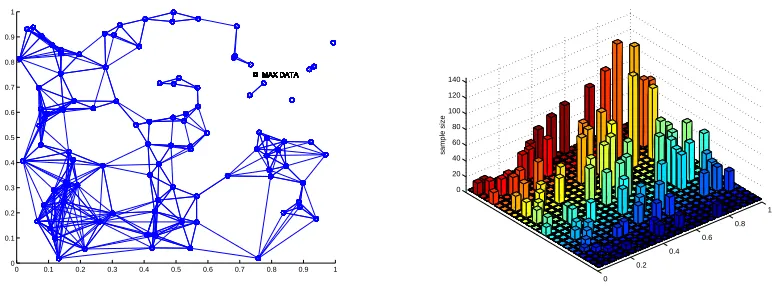
Figure 1: Visual illustration of Theorem 6.

In Figure 1 we provide a visual illustration of the behavior of Theorem 3 applied to a simple clas-sification problem. In this problem there are K=100 classifiers, each classifier fifor i=1. . .100 is

defined by 2 parameters represented by a point in the unit square, such that the expected disagree-ment rate between two such classifiers is proportional the L1 distance between their parameters.2

We chose the 100 parameter vectors fi uniformly at random from the unit square (the circles in

the left panel). To generate varying source sizes, we let ni decrease with the distance of fi from a

chosen “central” point at(0.75,0.75)(marked “MAX DATA” in the left panel); the resulting source sizes for each model are shown in the bar plot in the right panel, where the origin(0,0)is in the near corner,(1,1) in the far corner, and the source sizes clearly peak near(0.75,0.75). For every function fi we used Theorem 6 to find the best sources j to be used to estimate its parameters. The

undirected graph on the left includes an edge between fi and fj if and only if the data from fj is

used to learn fiand/or the converse.

The graph simultaneously displays the geometry implicit in Theorem 6 as well as its adaptivity to local circumstances. Near the central point, the graph is sparse and the edges quite short, corre-sponding to the fact that for such models we have enough direct data (represented with high bars in the right panel) that it is not advantageous to include data from distant models. Far from the central point the graph becomes dense and the edges long, as we are required to aggregate a larger neighborhood to learn the optimal model. In addition, decisions are affected locally by how many models are “nearby” a given model, when there are many close functions fj to a given fi there is

no need to use “far” models, but when the neighborhood of a function is not populated with many examples, there is a need for data from models far-away.

5. Bounds Using Rademacher Complexity

Given the interest in tighter, potentially data-dependent convergence bounds (such as maximum margin bounds, PAC-Bayes, and others) in recent years, it is natural to ask how our multi-source theory can exploit these modern bounds. We examine one specific case here using Rademacher

2. It is easy to create simple input distributions and classifiers that generate exactly this geometry. Let the input x be a pair x= (p,b)where p∈[0,1],b∈ {0,1}and let the hypothesis class consist of functions defined as pairs of thresholds f = (t1,t2)where f(x) =1 if and only if (p>t1and b=0) or (p>t2and b=1). The distribution of

complexity (Bartlett and Mendelson, 2002; Bartlett et al., 2002; Koltchinskii, 2001; Koltchinskii and Panchenko, 2000); analogs can be derived in a similar manner for other complexity measures. We start by deriving bounds for settings in which generic Lipschitz loss functions are used, and then discuss specific applications to classification and to regression with squared loss.

5.1 Rademacher Complexity and General Lipschitz-loss Bounds

If

H

is a class of functions mapping from a set

X

toR, the empirical Rademacher complexity of

H

on a fixed set of observations x1, . . . ,xnis defined as

ˆ

Rn(

H

) =E

"

sup

h∈H

2 n

n

∑

i=1

σih(xi)

#

,

where the expectation is taken with respect to independent uniform _{±1_}-valued random vari-ablesσ1, . . . ,σn. The Rademacher complexity for n observations can then be defined as Rn(

H

) =

ERˆn(

H

)

where the expectation is with respect to observations x1, . . . ,xn. In the standard setting,

x1, . . . ,xn are drawn i.i.d. from a fixed distribution. In our setting, these observations will still be

independent, but not necessarily identically distributed. We will show that the standard uniform convergence results still hold for this modified definition of Rademacher complexity.

Consider any setting in which each generalized data point z=_hx,y_ifor some x_∈

X

and y_∈

Y

with y= f(x). A cost function for the loss

L

is a functionφ(y,a):R→Rsuch that

L

(h,_hx,y_i) =

φ(y,h(x))for all x_∈

X

, y_∈

Y

, and h_∈

H

. We will consider cost functionsφthat are Lipschitz in the second parameter. Defineφ0(y,a) =φ(y,a)₋φ(y,0). Note that if φis Lipschitz in the second parameter with constant L thenφ0is also Lipschitz in the second parameter with the same constant L.

Lemma 8 below gives a uniform convergence bound for any loss function with a corresponding Lipschitz cost function. The proof of this lemma is in Appendix A. It is analogous to the proof of Theorem 8 in Bartlett and Mendelson (2002), which makes a similar claim in the i.i.d. setting, and uses the following lemma from Bartlett and Mendelson (2002).

Lemma 7 Ifφ:R→Ris Lipschitz with constant L andφ(0) =0, then Rn(φ◦

H

)≤2LRn(

H

).

Lemma 8 Let

L

be a loss function bounded in [0,1], and φ:R→R a cost function such that

L

(f,_hx,y_i) =φ(y,f(x))where φ is Lipschitz in the second parameter with constant L. Let

H

:

X

→

Y

be a class of functions and let_{hxi,yii}ni=1 be sampled independently according to some

probability distributed P. For any n, for any 0<δ<1, with probability 1₋δ over samples of length n, every h_∈

H

satisfies

β(n,δ) =2LRn(

H

) +

r

2 ln(2/δ)

n .

5.2 Application to Classification Using Rademacher Complexity

Theorem 9 below follows from the application of Theorem 3 using the 1-triangle inequality and an application of Lemma 8 with

φ(y,a) =

  

 

1 if ya_≤0,

Notice first that if

L

is the 0/1 loss, then for all x∈

X

, y ∈ {−1,1}, and h∈

X

→ {−1,1},

L

(h,_hx,y_i) =φ(y,h(x)), and furthermore that φis Lipschitz with constant 1, so Lemma 8 can be applied immediately.

Theorem 9 Let

F

be a set of functions from an input set

X

into _{-1,1_} and let Rn1:k(

H

) be the

Rademacher complexity of

H

_⊆

F

on the first k sources of data. Let e be the expected 0/1 loss. Let K, f =f1,f2, . . . ,fK∈

F

,{εi}K_i=1,{ni}K_i=1, and ˆhk be defined as in the multi-source learning model.

For anyδsuch that 0<δ<1, with probability at least 1₋δ, for any k_{∈ {}1, . . . ,K_}

e(f,ˆhk)≤min

h∈H{e(f,h)}+2 k

∑

i=1

ni

n1:k

εi+2

s

2 ln(4K/δ)

n1:k

+4Rn1:k(

H

).

Before moving on, let us briefly examine the behavior of this bound. Similarly to the VC-based bound given in Theorem 6, as k increases and more sources of data are combined, the second term will grow while the third will shrink. The behavior of the final term Rn1:k(

H

), however, is less predictable and may grow or shrink as more sources of data are combined.

Note that for the special case of classification with 0/1 loss, it is possible to get tighter bounds with better dependence on Rn1:k by using a more careful analysis than the one in the proof of Lemma 8. Such bounds are given in an earlier version of this paper (Crammer et al., 2007); we choose not to present these alternate bounds here to simplify presentation.

5.3 Regression

We now turn to (noise-free) regression with squared loss. Here our target model f is any function from an input class

X

into some bounded subset ofR. (Frequently we will have

X

_⊆Rd, but this is not required.) Our loss function is

L

(h,_hx,yi) = (y−h(x))2_{, and the expected loss is thus}

e(g1,g2) =E_hx,yi∼P_g1[

L

(g2,hx,yi)] =Ex_∼P

(g1(x)−g2(x))2

.

For regression it is known that the standard 1-triangle inequality does not hold. However, a 2-triangle inequality does hold and is stated in the following lemma.

Lemma 10 Given any three functions g1,g2,g3:

X

→R, a fixed and unknown distribution P on the

inputs

X

, and the expected loss e(g1,g2) =Ex∼P

(g1(x)−g2(x))2

,

e(g1,g2)≤2(e(g1,g3) +e(g3,g1)).

Proof: By Jensen’s inequality and the convexity of x_7→x2, for any g1, g2, and g3,

e(g1,g2) = Ex∼P

(g1(x)−g2(x))2

= Ex∼P

"

4

1

2(g1(x)−g3(x)) + 1

2(g3(x)−g2(x))

2#

≤ Ex_∼P

2(g1(x)−g3(x))2+2(g3(x)−g2(x))2

=2(e(g1,g3) +e(g3,g1)) .

Lemma 11 Let

H

:

X

→[₋B,B]be a class of functions, and let

L

(h,_hx,yi) = (y−h(x))2 _{be the}

squared loss. The following functionβis a uniform convergence bound for

H

and

L

:

β(n,δ) =8BRn(

H

) +4B2

r

2 ln(2/δ)

n .

Proof: We cannot apply Lemma 8 directly using the squared loss function, since it may output values outside of the range[0,1]. Instead, we apply the Lemma 8 using the alternate loss function

L

0_{(h,hx,yi) =φ(y,h(x))where}

φ(y,a) =

  

 

1

4B2(y+B)2 if a<−B, 1

4B2(y−a)2 if−B≤a≤B, 1

4B2(y+B)2 if a>B.

It is easy to see thatφalways outputs values in the range[0,1]. Furthermore, for any y_∈[₋B,B],φ is Lipschitz in the second parameter with parameter 1/B. For any[a,b]_∈[₋B,B],

|φ(y,a)₋φ(y,b)_| = 1

4B2

(y−a)2−(y−b)2 =

1 4B2

a2−b2+2y(b−a)

≤ _4B1₂ a2−b2

+

1

2B2|y(a−b)|

≤ 1

4B2|a+b||a−b|+

1

2B2|y(a−b)| ≤

1

B|a−b|.

Applying Lemma 8 gives a uniform convergence bound of(2/B)Rn(

H

) +

p

2 ln(2/δ)/n for

L

0. Scaling by 4B2yields the bound for

L

.

Combining this with Lemma 10 and applying Theorem 3 yields the following.

Theorem 12 Let

F

be the set of functions from

X

into[₋B,B], and

H

_⊆

F

. Let e be the expected squared loss. Let K, f =f1,f2, . . . ,fK∈

F

,{εi}Ki=1,{ni}Ki=1, and ˆhkbe defined as in the multi-source

learning model. For anyδsuch that 0<δ<1, with probability at least 1₋δ, for any k_{∈ {}1, . . . ,K_}

e(f,ˆhk)≤4 min

h∈H{e(f,h)}+6 k

∑

i=1

ni

n1:k

εi+32BRn1:k(

H

) +16B

2

s

2 ln(4K/δ)

n1:k

.

5.4 Remarks on the Use of Data-Dependent Complexity Measures

The following lemma, which relates the true Rademacher complexity of a function class to its empirical Rademacher complexity, follows directly from Theorem 11 of Bartlett and Mendelson (2002), the proof of which does not require samples to be identically distributed.

Lemma 13 Let

H

be a class of functions mapping to[₋1,1]. For any integer n, for any 0<δ<1, with probability 1₋δ,

R_n(

H

)−Rˆ_n(

H

) ≤

r

8 ln(2/δ)

This lemma immediately allows us to replace Rn(

H

)with that data-dependent quantity ˆRn in

any of the bounds above for only a small penalty.

While the use of data-dependent complexity measures can be expected to yield more accurate bounds and thus better decisions about the number k∗ of sources to use, it is not without its costs in comparison to the more standard data-independent approaches. In particular, in principle the optimization of a data-dependent version of the bound given in Theorem 9 to choose k∗may actually involve running the learning algorithm on all possible prefixes of the sources, since we cannot know the dependent complexity term for each prefix without doing so. In contrast, the data-independent bounds can be computed and optimized for k∗without examining the data at all, and the learning performed only once on the first k∗ sources. This is especially useful in the case that labels are not free but must be purchased at a price.

6. Estimating the Disparity Matrix

A potential drawback of the theory presented here is the need to estimate the disparity matrix D when it is unknown. However, it is often the case that this matrix can be estimated with many fewer labeled samples than are required for learning. In this section, we discuss how D can be estimated in the classification setting.

As before, consider the scenario in which each target function is a fixed, unknown and arbitrary function from some input set

X

to{−1,1}, and assume that there is a fixed and unknown distribution P over

X

. Suppose we are given m data points labeled by a pair of functions fiand fj, and let ˆe(fi,fj)

be the fraction of points on which the labels disagree. By Hoeffding’s inequality, with probability 1₋δ0,

|eˆ(fi,fj)−e(fi,fj)| ≤

r

ln(2/δ0₎

2m .

Thus in order to approximate e(fi,fj)with an error no more thanε, only ln(2/δ0)/(2ε2)commonly

labeled points are needed. Applying the union bound gives us the following lemma.

Lemma 14 Let

F

be a set of functions from

X

into_{−1,1_}, and suppose f1, . . . ,fK∈

F

. Let e be

the expected 0/1 loss. Suppose that for each pair i,j_{∈ {}1,_···,K_}, there exist mi,j≥m0examples

distributed according to P commonly labeled by fiand fj, where

m0=

2 ln(K) +ln(2/δ)

2ε2

for anyδsuch that 0_≤δ_≤1, and let ˆe(fi,fj)be the fraction of commonly labeled examples on which

fi and fj disagree. Then with probability 1−δ, for all i,j∈ {1,···,K},|eˆ(fi,fj)−e(fi,fj)| ≤ε.

Using the lemma we set the upper bound on the mutual error e(fi,fj)between the pair of

func-tion fiand fj to be Di,j=eˆ(fi,fj) +ε. With probability at least 1−δthese bound holds

simultane-ously for all i,j.

Note that in general, log(K)will be significantly smaller than the dimension d of

H

. Thus many fewer labeled examples are required to estimate the disparity matrix than to actually learn the best function in the class.

certain movies using ratings from other users. It is often the case that pairs of users will have seen many of the same movies. These commonly rated movies can be used to determine how similar each pair of users are, while ratings of additional movies can be reserved to learn the prediction functions.

7. Estimating the Parameters of a Distribution

We now proceed with the study of the related problem of estimating the unknown parameters of a distribution from multiple sources of data. As in the previous sections, we provide a bound on the diversity of an estimator based on the first k sources from the target. Up until this point, we have measured the diversity between two functions by using the expected value of a loss function. The loss is a function of two specific observations. Thus, although two functions may not agree on many points, the diversity between them could be zero (if the measure of their disagreement points is zero). In this section we use a more direct way to measure the diversity between two functions by computing the distance between the parameters used to specify these distributions.

Before stating the problem formally we provide with some illustrative examples for intuition.

Example 1 We wish to estimate the bias θ of a coin given K sources of training observations N1, ...,NK. Each source Nk contains nk outcomes of flips of a coin with bias θk. The only

infor-mation we are given is thatθk∈[θ−εk,θ+εk].

In the next example we consider the simple generalization to the multinomial distribution, which involves more than a single parameter.

Example 2 We wish to estimate the probabilityΘ(p)of a die to fall on its pth side (out of D possible outcomes) given K sources of training observations N1, ...,NK. Each source Nkcontains nkoutcomes

using a die with parameters Θ(_kp). The only information provided is a bound on the `∞distance between the parameter sets, maxp|Θ(

p)

k −Θ(p)|=kΘk−Θk∞≤εk.

Formally, let Pr[X_|Θ]be a parametric family of distributions such that X_∈Rd andΘ_∈RD. We assume that there exists a vector functionΨsuch that

E

h

Ψ(p)_(X)i_=Θ(p) _{for p=1, . . . ,D.}

This assumption is met, for example, by any member of the exponential family. In the two examples we have discussed, the functionΨis simply an identity or indicator. This function is useful because it allows us to estimate the parameters of the distribution from data. Let X1,···,Xn be a sequence

of n i.i.d. samples from such a distribution, where the functionΨis known. Then the estimator obtained by the method of moments is given by the empirical mean

ˆ

Θ=1

n

n

∑

i=1

Ψ(Xi).

In our setting, we wish to estimate the parametersΘof a parametric distribution Pr[X_|Θ]given K sources of training observations N1, ...,NK. Each source Nkcontains nkoutcomes from a distribution

with parametersΘk, that is, Pr[X|Θk]. The only information we are given is a bound on the `∞

We first bound the deviation of this estimation from the true parameters using Hoeffding’s in-equality. Fix the value of the index p=1, . . . ,D. We assume that there exist A and B>0 such that,

Ψ(p)_(X

i)∈[A,A+B] for i=1, . . . ,n.

Then, Pr h E h ˆ

Θ(p)i_−Θˆ(p) ≥ε

i

≤2 exp

−2nε

2

B2

.

Setting the right hand-side of the inequality equal toδand solving forε, we get

Pr   E h ˆ

Θ(p)i

−Θˆ(p) ≥

s

B2_ln(2

δ) 2n



≤δ.

We can use the union bound to bound on this difference for all D parameters at once and get

Pr



∃p : E

h

ˆ

Θ(p)i

−Θˆ(p) ≥

s

B2_ln(2D

δ ) 2n  ≤ D

∑

p=1

δ

D=δ.

This proves the following lemma.

Lemma 15 Let X1, . . . ,Xn be a sequence of i.i.d. random variables. Let ˆΘ= 1_n∑ni=1Ψ(Xi) and

Θ=EΘˆ, where both ˆΘandΘare D-dimensional vectors. Assume thatΨ(p)(Xi)∈[A,A+B]for

i=1, . . . ,n, p=1, . . . ,D, for some A and B>0. Then, for anyδ_∈(0,1)the following bound holds.

Pr



kΘ−Θˆk∞≥ s

B2_ln(2D

δ ) 2n



≤δ.

We now turn our attention to the problem of choosing the best sources. We define the estimator using the first k sources to be,

ˆ

Θk=

1 n1:k

k

∑

i=1X

∑

∈Ni

Ψ(X),

where as before n1:k=∑ki=1ni. We denote the expectation of this estimate by

¯

Θk=E

Θ_ˆ k = 1 n1:k k

∑

i=1

niΘi.

We now bound the deviation of the estimate ˆΘk from the true set of parametersΘusing the

expec-tation ¯Θk,

kΘ−Θˆkk∞ = kΘ−Θ¯k+Θ¯k−Θˆkk∞ ≤ kΘ−_Θ¯_kk∞+kΘ¯_k−Θˆ_kk∞ ≤

k

∑

i=1

nikΘ−Θik∞

n1:k

+_kΘ¯k−Θˆkk∞

≤ k

∑

i=1

ni

n1:k

10 20 30 0

0.5 1

10 20 30

0 0.5 1

10 20 30

0 0.5 1

10 20 30

0 0.5 1

10 20 30

0 0.5 1

10 20 30

0 0.5 1

10 20 30

0 0.5 1

10 20 30

0 0.5 1

10 20 30

0 0.5 1

10 20 30

0 0.5 1

10 20 30

0 0.5 1

10 20 30

0 0.5 1

10 20 30

0 0.5 1

10 20 30

0 0.5 1

10 20 30

0 0.5 1

10 20 30

0 0.5 1

10 20 30

0 0.5 1

10 20 30

0 0.5 1

10 20 30

0 0.5 1

10 20 30

0 0.5 1

10 20 30

0 0.5 1

10 20 30

0 0.5 1

10 20 30

0 0.5 1

10 20 30

0 0.5 1

10 20 30

0 0.5 1

10 20 30

0 0.5 1

10 20 30

0 0.5 1

10 20 30

0 0.5 1

10 20 30

0 0.5 1

10 20 30

0 0.5 1

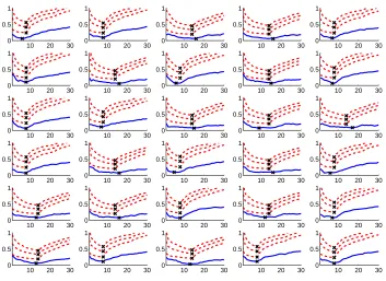
Figure 2:Simulation of the multiple source error bounds.

Let B=maxk=1...Ksup XkΨ(X)k∞. We can then use Lemma 15 to bound the second term above,

yielding the following theorem.

Theorem 16 Let ˆΘk be the estimate ofΘobtained by using only the data from the first k sources,

where both ˆΘand Θare D-dimensional vectors. Assume that ₋B_≤Ψ(p)(Xi)≤B. Then for any

δ>0, with probability_≥1₋δwe have

kΘ−Θˆkk∞≤ k

∑

i=1

ni

n1:k

εi+

s

4B2_ln(2DK

δ ) 2n1:k

simultaneously for all k=1, . . . ,K.

As we did with Theorem 3, we can convert Theorem 16 into an algorithm for selecting data sources. Given the K sources of data we simply compute the bounds provided by these theorems for each prefix of the sources of length k and select the subset of sources that yields the smallest bound. A bound for the special case of Example 1 was developed and presented in previous work (Crammer et al., 2006). That bound has the same form as the bound given here in Theorem 16 but with better constants.

8. Synthetic Simulations

goal is to learn thirty classifiers from this class using only limited amounts of data. These data points are drawn uniformly at random from inside the 15-dimensional unit sphere. In this restricted setting, it is easy to calculate the disparity between two functions. Representing each function f by a unit weight vector w such that f(x) =sign(w·x), the distance between functions w and w0 is simplyθ/πwhereθ=arccos(w_·w0)is the angle between w and w0.

In each simulation we ran, the linear classifiers were generated as follows. First, three base classifiers were generated by choosing weight vectors uniformly at random from the surface of the 15-dimensional sphere. Each of the thirty classifiers was then generated by randomly choosing one of the base classifiers, perturbing each coordinate of its weight vector, and renormalizing the perturbed weights.

The number of training samples available for each function was generated from a Poisson dis-tribution with a mean of 8. Each data instance was then sampled from inside the 15-dimensional unit sphere via rejection sampling and labeled by the corresponding classifier, and 500 test samples for each function were generated in the same manner.

To predict the optimal set of training data sources to use for each model, we calculated an approximation of the multiple-source VC bound for classification. It is well known that the constants in the VC-based uniform convergence bounds are not tight. Thus for the purpose of illustrating how these bounds might be used in practice, we have chosen to show approximations of our bounds with a variety of constants. In particular, we have chosen to approximate the bound with

2

k

∑

i=1

nk

n1:K

εk+C

s

(d ln(2en1:K/d) +ln(8K/δ))

n1:K

withδ=0.001 for different values of C. These approximations yield curves that are closer in shape and magnitude to the actual error than a curve generated using the precise, overly conservative constants of Theorem 6.

The set of plots shown in Figure 2 illustrates the results of a single multiple source simulation. (Results from repeated versions of this experiment and experiments with different source sizes were similar.) Each individual plot represents a particular target function. On the x axis is the number of data sources used in training. On the y axis is error. The solid blue curves show test error of a model trained using logistic regression. Dashed red curves show our multiple source error bound with C set to 1/4 in the lowest curve, 1/2 in the middle curve, and 1/√2 in the highest curve. The_×on each curve marks the minimum value.

These plots clearly show the trade-off that exists. When too few sources are used, there is not enough data available to learn a 15-dimensional function. When too many sources are used, the labels on the training data often will not correspond to the labels that would have been assigned by the target function. The optimal amount of data lies somewhere in between.

Acknowledgments

We thank the anonymous reviewers for many valuable suggestions, especially on the simplified presentation of the application to regression.

Appendix A. Proof of Lemma 8

The proof relies on McDiarmid’s inequality (McDiarmid, 1989), which is stated here for complete-ness.

Lemma 17 (McDiarmid’s inequality) Let x1, . . . ,xn be independent random variables taking on

values in a set A and assume that f : An_→Rsatisfies sup

x1,...,xn,x0i∈A

|f(x1, . . . ,xn)−f(x1, . . . ,xi−1,xi0,x_i+1, . . . ,x_n)| ≤c_i

for every 1_≤i_≤n. Then for every t>0,

Pr[f(x1, . . . ,xn)−E[f(x1, . . . ,xn)]≥t]≤exp−2t 2_/∑n

i=1c2i _.

Here we show one direction of the bound, namely that with probability 1₋δ/2, for all h_∈

H

,

e(h)_≤eˆ(h) +2LRn(

H

) +

r

2 ln(2/δ)

n .

The proof of the other direction is nearly identical. For i_{∈ {}1, . . . ,n_}, let_hxi,yii be the ith

train-ing instance, distributed accordtrain-ing to Pi, and lethx0i,y0ii be independent random variables drawn

according to Pi. Note that for all h∈

H

,

e(h) = e(h) +eˆ(h)₋eˆ(h)_≤eˆ(h) + sup

h0_∈H

e(h0)₋eˆ(h0)

= eˆ(h) + sup

h0_∈H E_{hx0

i,y0ii}ni=1

"

1 n

n

∑

i=1

φ(y0_i,h0(x0_i))

#

−1_n n

∑

i=1

φ(yi,h0(xi))

!

= eˆ(h) + sup

h0_∈H E_{hx0

i,y0ii}ni=1

"

1 n

n

∑

i=1

φ0_(y0

i,h0(x0i)) +φ(y0i,0)

#

−1_n n

∑

i=1

φ0_(y

i,h0(xi)) +φ(yi,0)

!

.

When only one instance_hxi,yiichanges, the sup term can change by at most 2/n. Thus we can

apply McDiarmid’s inequality to see that with probability at least 1−δ/2,

e(h)_≤eˆ(h) +E

"

sup

h0_∈H E

"

1 n

n

∑

i=1

φ0_(y0

i,h0(x0i))

#

−1_n n

∑

i=1

φ0_(y

i,h0(xi))

!#

+

r

2 ln(2/δ)

n ,

where the outer expectation is with respect to set of training instances_{hxi,yii}n_i=1 and the inner

this middle term is bounded by 2LRn(

H

). Using the fact that the supremum of an expectation is

less than or equal to the expectation of a supremum, we find that

E_{hxi,yii}ni=1

"

sup

h0_∈H

E_{hx0_i,y0_ii}n i=1

"

1 n

n

∑

i=1

φ0_(y0 i,h0(x0i))

#

−1_n n

∑

i=1

φ0_(y

i,h0(xi))

!#

≤ E_{hxi,yii}ni=1,{hx0i,y0ii}ni=1

"

sup

h0_∈H 1 n

n

∑

i=1

φ0_(y0

i,h0(x0i))−φ0(yi,h0(xi))

#

= E_{hxi,yii}ni=1,{hx0i,y0ii}ni=1,{σi}ni=1

"

sup

h0_∈H 1 n

n

∑

i=1

σi φ0(y0i,h0(xi0))−φ0(yi,h0(xi))

#

≤ E_{hxi,yii}ni=1,{σi}ni=1

"

sup

h0_∈H 2 n

n

∑

i=1

σiφ0(yi,h0(xi))

#

=Rn(φ0◦

H

).

Lemma 7 implies that Rn(φ0◦

H

)≤2LRn(

H

)sinceφis Lipschitz with parameter L. The result

follows.

References

M. Anthony and P. Bartlett. Neural Network Learning: Theoretical Foundations. Cambridge Uni-versity Press, 1999.

P. Bartlett and S. Mendelson. Rademacher and Gaussian complexities: Risk bounds and structural results. Journal of Machine Learning Research, 3:463–482, 2002.

P. Bartlett, S. Boucheron, and G. Lugosi. Model selection and error estimation. Machine Learning, 48:85–113, 2002.

J. Baxter. Learning internal representations. In Proceedings of the Eighth Annual Conference on Computational Learning Theory, 1995.

S. Ben-David. Exploiting task relatedness for multiple task learning. In Proceedings of the Sixteenth Annual Conference on Computational Learning Theory, 2003.

J. Blitzer, K. Crammer, A. Kulesza, F. Pereira, and J. Wortman. Learning bounds for domain adaptation. In Advances in Neural Information Processing Systems 20, 2007.

K. Crammer, M. Kearns, and J. Wortman. Learning from data of variable quality. In Advances in Neural Information Processing Systems 18, 2006.

K. Crammer, M. Kearns, and J. Wortman. Learning from multiple sources. In Advances in Neural Information Processing Systems 19, 2007.

D. Haussler. Decision theoretic generalizations of the PAC model for neural net and other learning applications. Information and Computation, 100(1):78–150, 1992.

V. Koltchinskii. Rademacher penalties and structural risk minimization. IEEE Transactions on Information Theory, 47(5):1902–1914, 2001.

V. Koltchinskii and D. Panchenko. Rademacher processes and bounding the risk of function learn-ing. High Dimensional Probability, II:443–459, 2000.

A. Maurer. Algorithmic stability and meta-learning. Journal of Machine Learning Research, 6: 967–994, 2005.

C. McDiarmid. On the method of bounded differences. Surveys in Combinatorics, pages 148–188, 1989.

V. Vapnik. Statistical Learning Theory. Wiley, 1998.