Model Selection in Kernel Based Regression using the Influence Function

Model Selection in Kernel Based Regression using the Influence

Function

Michiel Debruyne [email protected]

Mia Hubert [email protected]

Department of Mathematics - LStat K.U.Leuven

Celestijnenlaan 200B, B-3001 Leuven, Belgium

Johan A.K. Suykens [email protected]

ESAT-SCD/SISTA K.U.Leuven

Kasteelpark Arenberg 10, B-3001 Leuven, Belgium

Editor: Isabelle Guyon

Abstract

Recent results about the robustness of kernel methods involve the analysis of influence functions. By definition the influence function is closely related to leave-one-out criteria. In statistical learn-ing, the latter is often used to assess the generalization of a method. In statistics, the influence function is used in a similar way to analyze the statistical efficiency of a method. Links between both worlds are explored. The influence function is related to the first term of a Taylor expan-sion. Higher order influence functions are calculated. A recursive relation between these terms is found characterizing the full Taylor expansion. It is shown how to evaluate influence functions at a specific sample distribution to obtain an approximation of the leave-one-out error. A specific implementation is proposed using a L1loss in the selection of the hyperparameters and a Huber loss

in the estimation procedure. The parameter in the Huber loss controlling the degree of robustness is optimized as well. The resulting procedure gives good results, even when outliers are present in the data.

Keywords: kernel based regression, robustness, stability, influence function, model selection

1. Introduction

Quantifying the effect of small distributional changes on the resulting estimator is a crucial analysis on many levels. A simple example is leave-one-out which changes the sample distribution slightly by deleting one observation. This leave-one-out error plays a vital role for example in model se-lection (Wahba, 1990) and in assessing the generalization ability (Poggio et al. 2004 through the concept of stability). Most of these analyses however are restricted to the sample distribution and the addition/deletion of some data points from this sample.

classifica-tion and regression. In Secclassifica-tion 3 these results are stated and their importance is summarized. A new theoretical result concerning higher order influence functions is presented. In Section 4 we show how to evaluate the resulting expressions at sample distributions. Moreover we apply these influ-ence functions in a Taylor expansion approximating the leave-one-out error. In Section 5 we use the approximation with influence functions to select the hyperparameters. A specific implementation

is proposed to obtain robustness with a Huber loss function in the estimation step and a L1loss in

the model selection step. The degree of robustness is controlled by a parameter that can be chosen in a data driven way as well. Everything is illustrated on a toy example and some experiments in Section 6.

2. The Influence Function

In statistics it is often assumed that a sample of data points is observed, all generated independently from the same distribution and some underlying process, but sometimes this is not sufficient. In many applications gathering the observations is quite complex, and many errors or subtle changes can occur when obtaining data. Robust statistics is a branch of statistics that deals with the detection and neutralization of such outlying observations. Roughly speaking a method is called robust if it produces similar results as the majority of observations indicates, no matter how a minority of other observations is placed. A crucial analysis in robust statistics is the behavior of a functional T , not only at the distribution of interest P, but in an entire neighborhood of distributions around P. The influence function measures this behavior. In this section we recall its definition and discuss some links with other concepts.

2.1 Definition

The pioneering work of Hampel et al. (1986) and Huber (1981) considers distributions Pε,z=

(1₋ε)P+ε∆z where ∆z denotes the Dirac distribution in the point z∈

X

Y

contaminated part of the data. For having a robust T , T(Pε,z)should not be too far away from T(P)

for any possible z and any smallε. The limiting case ofε_↓0 is comprised in the concept of the

influence function.

Definition 1 Let P be a distribution. Let T be a functional T : P_→T(P). Then the influence function of T at P in the point z is defined as

IF(z; T,P) =lim

ε→0

T(P_ε,z)−T(P)

ε .

The influence function measures the effect on the estimator T when adding an infinitesimally small amount of contamination at the point z. Therefore it is a measure of the robustness of T . Of particular importance is the supremum over z. If this is unbounded, then an infinitesimally small amount of contamination can cause arbitrary large changes. For robust estimators, the supremum of its influence function should be bounded. Then small amounts of contamination cannot completely change the estimate and a certain degree of robustness is indeed present. The simplest example is the estimation of the location of a univariate distribution with density f symmetric around 0. The

influence function of the mean at z_∈R _{then equals the function z and is clearly unbounded. If}

the median of the underlying distribution is uniquely defined, that is if f(0)>0, then the influence

function of the median equals sign(z)/(2 f(0))which is bounded. The median is thus more robust

2.2 Asymptotic Variance and Stability

From Definition 1 one can see that the influence function is a first order derivative of T(Pε,z) at

ε=0. Higher order influence functions can be defined too:

Definition 2 Let P be a distribution. Let T be a functional T : P_→T(P). Then the k-th order influence function of T at P in the point z is defined as

IFk(z; T,P) =

∂

∂kεT(Pε,z)|ε=0.

If all influence functions exist then the following Taylor expansion holds:

T(Pε,z) =T(P) +εIF(z; T,P) +

ε2

2!IF2(z; T,P) +. . . (1) characterizing the estimate at a contaminated distribution in terms of the estimate at the original distribution and the influence functions.

Actually this is a special case of a more general Von Mises expansion (take Q=P_ε,z):

T(Q) =T(P) + Z

IF(x; T,P)d(Q₋P)(x) +. . .

Now take Q equal to a sample distribution Pn of a sample{zi} of size n generated i.i.d. from P.

Then

T(Pn)−T(P) = Z

IF(z; T,P)dPn(z) +. . .

=1

n

n

∑

IF(zi; T,P) +. . . .

The first term on the right hand side is now a sum of n i.i.d. random variables. If the remaining terms

are asymptotically negligible, the central limit theorem thus immediately shows that √n(T(Pn)−

T(P))is asymptotically normal with mean 0 and variance

ASV(T,P) = Z

IF2(z; T,P)dP(z).

Since the asymptotic efficiency of an estimator is proportional to the reciprocal of the asymptotic variance, the integrated squared influence function should be as small as possible to achieve high efficiency. Consider again the estimation of the center of a univariate distribution with density f . At

a standard normal distribution the asymptotic variance of the mean equalsR

z2_{dP(z) =1, and that}

of the median equalsR

(sign(z)/(2 f(0)))2_{dP(z) =1.571. Thus the mean is more efficient than the}

median at a normal distribution. However, at a Cauchy distribution for instance, this is completely different: the ASV of the median equals 2.47, but for the mean it is infinite since the second moment of a Cauchy distribution does not exist. Thus to estimate the center of a Cauchy, the median is a much better choice than the mean.

and Niyogi, 2002) and CVloo-stability (Poggio et al., 2004). The basic idea is that the result of a

learning map T on a full sample should not be very different from the result obtained when removing

only one observation. More precisely, let P be a distribution on a set

X

Y

T(P):

X

Y

ith observation zi = (xi,yi)∈

X

Y

function L :

Y

lim

n→∞_i∈{sup_1,...,n}|L(yi−T(Pn)(xi))−L(yi−T(P −i

n )(xi))| →0 (2)

for n_→∞. This means intuitively that the prediction at a point xishould not be too different whether

or not this point is actually used constructing the predictor. If the difference is too large there is no stability, since in that case adding only one point can yield a large change in the result. Under

mild conditions it is shown that CVloo-stability is required to achieve good predictions. Let L be the

absolute value loss and consider once again the simple case of estimating the location of a univariate

distribution. Thus Pnis just a univariate sample of n real numbers{y1, . . . ,yn}. Then the left hand

side of (2) equals

lim

n→∞_i∈{sup_1,...,n}|T(Pn)−T(P −i n )|.

Let y(i)denote the ith order statistic. Consider T the median. Assuming that n is odd and yi<y₍n+1 2 )

(the cases yi>y₍n+1

2 )and equality can easily be checked as well), we have that

|Med(Pn)−Med(Pn−i)|=

y₍n+1 2 )−

1 2

y₍n+1

2 )+y(

n+3 2 )

=1

2|y(n+21)−y(

n+3 2 )|.

If the median of the underlying distribution P is unique, then both y₍n+1

2 )and y(

n+3

2 )converge to this

number and CVloostability is obtained. However, when taking the mean for T , we have that

|E_(Pn)−E_(Pn−i_)|= 1 n n

∑

yj−

1

n−1

n

∑

j=1

j6=i

yj = − 1

n(n−1) n

∑

j=1

j6=i

yj+

yi n .

The first term in this sum equals the sample mean of P_n−idivided by n and thus converges to 0 if the

mean of the underlying distribution exists. The second term converges to 0 if

lim

n→∞_i∈{sup_1,...,n} |yi|

n =0.

This means that the largest absolute value of n points sampled from the underlying distribution should not grow too large. For a normal distribution for instance this is satisfied since the largest observation only grows logarithmically: for example the largest of 1000 points generated from a normal distribution only has a very small probability to exceed 5. This is due to the exponentially decreasing density function. For heavy tailed distribution it can be different. A Cauchy density for instance only decreases at the rate of the reciprocal function and sup_{i∈{1,...,n}|}yi|is of the order O(n).

Thus for a normal distribution the mean is CVloostable, but for a Cauchy distribution it is not.

In summary note that both the concepts of influence function and asymptotic variance on one

an estimator is ok as long as the median of the underlying distribution is unique. Then one has CVloo

stability and a finite asymptotic variance. Using the sample mean is ok for a normal distribution,

but not for a Cauchy distribution (no CVloostability and an infinite asymptotic variance).

A rigorous treatment of asymptotic variances and regularity conditions can be found in Boos and Serfling (1980) and Fernholz (1983). In any event, it is an interesting link between perturba-tion analysis through the influence funcperturba-tion and variance/efficiency in statistics on one hand, and between leave-one-out and stability/generalization in learning theory on the other hand.

2.3 A Strategy for Fast Approximation of the Leave-one-out Error

In leave-one-out crossvalidation T(P_n−i) is computed for every i. This means that the algorithm

under consideration has to be executed n times, which can be computationally intensive. If the influence functions of T can be calculated, the following strategy might provide a fast alternative. First note that

P_n−i= (1₋( −1

n₋1))Pn+

−1

n₋1∆zi.

Thus, taking Pε,z=Pn−i,ε=−1/(n−1)and P=Pn, Equation (1) gives

T(P_n−i) =T(Pn) +

∞

∑

( −1

n₋1)

jIFj(zi; T,Pn)

j! . (3)

The right hand side now only depends on the full sample Pn. In practice one can cut off the series

after a number of steps ignoring the remainder term, or if possible one can try to estimate the remainder term.

The first goal of this paper is to apply this idea in the context of kernel based regression. Christ-mann and Steinwart (2007) computed the first order influence function. We will compute higher order terms in (1) and use these results to approximate the leave-one-out estimator applying (3).

3. Kernel Based Regression

In this section we recall some definitions on kernel based regression. We discuss the influence function and provide a theorem on higher order terms.

3.1 Definition

Let

X

Y

X

Y

of n observations(xi,yi)∈

X

Y

sample distribution. A functional T is a map that maps any distribution P onto T(P). A finite sample

approximation is given by Tn:=T(Pn).

Definition 3 A function K :

X

X

X

H

X

H

X

K(x,x0) = _hΦ(x),Φ(x0)_i.

Frequently used kernels include the linear kernel K(xi,xj) =xtixj, polynomial kernel of degree p

for which K(xi,xj) = (τ+xtixj)pwithτ>0 and RBF kernel K(xi,xj) =exp(−kxi−xjk2₂/σ2)with

bandwidthσ>0. By the reproducing property of

H

H

X

as the inner product of f with the feature map: f(x) =_hf,Φ(x)_i.

Definition 4 Let K be a kernel function with corresponding feature space

H

H

is defined by

f_λ,K,P:=argmin f∈H

E_{PL(Y−f(X)) +}λ_kfk2_H

whereλ>0 is a regularization parameter.

The functional f_λ,K maps a distribution P onto the function fλ,K,P that minimizes the regularized

risk. When the sample distribution Pnis used, one has that

f_λ,K,Pn :=argmin f∈H

1

n

n

∑

L(yi−f(xi)) +λkfk2_H. (4)

Such estimators have been studied in detail, see for example Wahba (1990), Tikhonov and Arsenin (1977) or Evgeniou et al. (2000). In a broader framework (including for example classification, PCA, CCA etc.) primal-dual optimization methodology involving least squares kernel estimators were studied by Suykens et al. (2002b). Possible loss functions include

• the least squares loss: L(r) =r2.

• Vapnik’sε-insensitive loss: L(r) =max_{|r_{| −}ε,0_}, with special case the L1loss ifε=0.

• the logistic loss: L(r) =₋log(4Λ(r)[1₋Λ(r)])withΛ(r) =1/(1+e−r). Note that this is not the same loss function as used in logistic regression.

• Huber loss with parameter b>0: L(r) =r2if_|r_{| ≤}b and L(r) =2b_|r_{| −}b2if_|r_|>b. Note

that the least squares loss corresponds to the limit case b_→∞.

3.2 Influence Function

The following proposition was proven in Christmann and Steinwart (2007).

Proposition 5 Let

H

X

X

H

X

Y

X

Y

IF(z; f_λ,K,P) =−S−1 2λfλ,K,P

+L0(zy−fλ,K,P(zx))S−1Φ(zx)

where S :

H

H

Thus if the kernel is bounded and the first derivative of the loss function is bounded, then the

influence function is bounded as well. Thus L1 type loss functions for instance lead to robust

1/(1+e−r) which is bounded by 2. For the Huber loss L0(r)is bounded by 2b. This shows that the parameter b controls the amount of robustness: if b is very large than the influence function can become very large too. For a small b the influence function remains small. For a least squares

loss function on the other hand, the influence function is unbounded (L0(r) =2r): the effect of the

smallest amount of contamination can be arbitrary large. Therefore it is said that the least squares estimator is not robust.

3.3 Higher Order Influence Functions

For the second order influence function as in Definition 2 the following theorem is proven in the Appendix.

Theorem 6 Let P be a distribution on

X

Y

all z := (zx,zy)∈

X

Y

IF2(z; f_λ,K,P) =S−1

2E_{P[IF(z; fλ,K,P)(X)L}00_{(Y−fλ,K(X))}Φ_(X)]

+E_{P[(IF(z; fλ,K,P)(X))}2_L000_{(Y−fλ,K,P(X))]}

−2[IF(z; f_λ,K,P)(zx)L00(zy−fλ,K(zx))Φ(zx)]

where S :

H

H

When the loss function is infinitely differentiable, all higher order terms can in theory be calculated, but the number of terms grows rapidly since all derivatives of L come into play. However, in the special case that all derivatives higher than three are 0, a relatively simple recursive relation exists.

Theorem 7 Let P be a distribution on

X

Y

X

Y

IFk+1(z; fλ,K,P) = (k+1)S−1

E_{P[IFk(z; fλ,K,P)(X)L}00_{(Y−fλ,K(X))}Φ_(X)]

−[IFk(z; fλ,K,P)(zx)L00(Zy−fλ,K(zx))Φ(zx)]

where S :

H

H

4. Finite Sample Expressions

Since the Taylor expansion in (1) is now fully characterized for any distribution P and any z, we

can use this to assess the influence of individual points in a sample with sample distribution Pn.

Applying Equation (3) with the KBR estimator f_λ,K,Pn from (4) we have that

f_λ,K,P−i

n (xi) =fλ,K,Pn(xi) +

∞

∑

( −1

n−1)

jIFj(zi; fλ,K,Pn)(xi)

j! . (5)

4.1 Least Squares Loss

First consider taking the least squares loss in (4). DenoteΩthe n_×n kernel matrix with i,j-th entry

equal to K(xi,xj). Let Inbe the n×n identity matrix and denote Sn=Ω/n+λIn. The value of fλ,K,Pn

at a point x_∈

X

f_λ,K,Pn(x) = 1

n

n

∑

αiK(xi,x) with

   α1 .. . αn   =S

−1 n    y1 .. . yn    (6)

which is a classical result going back to Tikhonov and Arsenin (1977). This also means that the vector of predictions in the n sample points simply equals



 

f_λ,K,Pn(x1) .. .

f_λ,K,Pn(xn)



 =H

   y1 .. . yn    (7)

with the matrix H=1_nS−_n1Ω, sometimes referred to as the smoother matrix.

To compute the first order influence function at the sample the expression in Proposition 5

should be evaluated at Pn. The operator S at Pnmaps by definition any f ∈

H

SPn(f) =2λf+EPn2 f(X)Φ(X) =2λf+ 2

n

n

∑

f(xj)Φ(xj)

and thus



 

SPn(f)(x1) .. .

SPn(f)(xn)



 =2λ



 

f(x1)

.. .

f(xn)

  + 2 n   

K(x1,x1) . . . K(x1,xn)

.. .

K(xn,x1) K(xn,xn)

     

f(x1)

.. .

f(xn)



 

=2Sn



 

f(x1)

.. .

f(xn)



 

which means that the matrix 2Snis the finite sample version of the operator S at the sample Pn. From

Proposition 5 it is now clear that



 

IF(zi; fλ,K,Pn)(x1)

.. .

IF(zi; fλ,K,Pn)(xn)



 =S

−1

n

(yi−fλ,K,Pn(xi))



 

K(xi,x1)

.. .

K(xi,xn)



 −λ



 

f_λ,K,Pn(x1) .. .

f_λ,K,Pn(xn)



 

. (8)

In order to evaluate the influence function at sample point zi at a sample distribution Pn, we only

need the full sample fit f_λ,K,Pn and the matrix S−

1

n , which is already obtained when computing fλ,K,Pn

recursively as



 

IFk+1(zi; fλ,K,Pn)(x1)

.. .

IFk+1(zi; fλ,K,Pn)(xn)





=(k+1)S

−1

n

Ω n



 

IF(zi; fλ,K,Pn)(x1)

.. .

IFk(zi; fλ,K,Pn)(xn)





 (9)

−(k+1)IFk(zi; fλ,K,Pn)(xi)S−n1



 

K(xi,x1)

.. .

K(xi,xn)



 .

Define[IFMk]the matrix containing IFk(zj; fλ,K,Pn)(xi)at entry i,j. Then (9) is equivalent to

[IFMk+1] = (k+1) (H[IFMk]−nH•[IFMk])

with_•denoting the entrywise matrix product (also known as the Hadamard product). Or

equiva-lently

[IFMk+1] = (k+1) (H([IFMk]•M(1−n))) (10)

with M the matrix containing 1/(1₋n)at the off-diagonal and 1 at the diagonal. A first idea is now

to approximate the series in (5) by cutting it off at some step k:

f_λ,K,P−i

n (xi)≈ fλ,K,Pn(xi) + k

∑

1

(1₋n)j_j![IFMj]i,i. (11)

However using (10) we can do a bit better. Expression (5) becomes

f_λ,K,P−i

n (xi) = fλ,K,Pn(xi) + 1

1₋n[IFM1]i,i+

1

1₋n[H(IFM1•M)]i,i

+ 1

1₋n[H(H(IFM1•M)•M)]i,i+. . .

In every term there is a multiplication with H and an entrywise multiplication with M. The latter means that all diagonal elements remain unchanged but the non-diagonal elements are divided by 1₋n. So after a few steps the non-diagonal elements will converge to 0 quite fast. It makes sense

to set the non-diagonal elements 0 retaining only the diagonal elements:

f_λ,K,P−i

n (xi)≈fλ,K,Pn(xi) + k−1

∑

1

(1−n)j_j![IFMj]i,i+

1

(1−n)k_k!

∞

∑

H_ij_,i[IFMk]i,i

=f_λ,K,Pn(xi) + k−1

∑

1

(1₋n)j_j![IFMj]i,i+

1

(1₋n)k_k!

[IFMk]i,i

1₋Hi,i

(12)

4.2 Huber Loss

For the Huber loss function with parameter b>0 we have that

L(r) =

(

r2 if_|r_|<b.

2b_|r_{| −}b2 _if|r|>b.

and thus

L0(r) =

(

2r if_|r_|<b

2b sign(r) if_|r_|>b , L

00_{(r) =}

(

2 if_|r_|<b

0 if_|r_|>b.

Note that the derivatives in_|r_|=b do not exist, but in practice the probability that a residual exactly

equals b is 0, so we further ignore this possibility. The following equation holds:

f_λ,K,Pn(x) = 1

n

n

∑

αiK(xi,x) with 2λαj=L0(yj−

1

n

n

∑

αiK(xi,xj)). (13)

Thus a set of possibly non-linear equations has to be solved inα. Once the solution for the full

sample is found, an approximation of the leave-one-out error is obtained in a similar way as for

least squares. Proposition 5 for Pngives the first order influence function.



 

IF(zi; fλ,K,Pn)(x1)

.. .

IF(zi; fλ,K,Pn)(xn)



 =S

−1

b

L0(yi−fλ,K,Pn(xi))



 

K(xi,x1)

.. .

K(xi,xn)



 −λ



 

f_λ,K,Pn(x1) .. .

f_λ,K,Pn(xn)



 

with Sb=2λIn+Ω•B/n and B the matrix containing L00(yi−fλ,K,Pn(xi)at every entry in the ith

column. Let Hb=S_b−1Ω/n•B. Starting from Theorem 7 one finds analogously as (10) the following

recursion to compute higher order terms.

[IFMk+1] = (k+1) (Hb([IFMk]•M(1−n))).

Finally one can use these matrices to approximate the leave-one-out estimator as

f_λ,K,P−i

n (xi)≈ fλ,K,Pn(xi) + k−1

∑

1

(1₋n)j_j![IFMj]i,i+

1

(1₋n)k_k!

[IFMk]i,i

1₋[Hb]i,i

(14)

in the same way as in (12)

4.3 Reweighted KBR

In Equation (14) the full sample estimator f_λ,K,Pn is of course needed. For a general loss function L

one has to solve Equation (13) to find f_λ,K,Pn. A fast way to do so is to use reweighted KBR with a

least squares loss. Let

W(r) = L0(r)

Then we can rewrite (13) as

2λf_λ,K,Pn(xk) = 1

n

n

∑

L0(yi−fλ,K,Pn(xi))K(xi,xk) ∀1≤k≤n.

=1

n

n

∑

2W(yi−fλ,K,Pn(xi))(yi−fλ,K,Pn(xi))K(xi,xk).

Denoting wi=W(yi−fλ,K,Pn(xi))this means that

λf_λ,K,Pn(xk) = 1

n

n

∑

wiyiK(xi,xk)−

1

n

n

∑

wifλ,K,Pn(xi)K(xi,xk) ∀1≤k≤n.

Let Iwdenote the n×n diagonal matrix with wiat entry i,i. Then



 

f_λ,K,Pn(x1) .. .

f_λ,K,Pn(xn)



 =

Ω

n +λIw −1Ω

n 

 

y1

.. .

yn





 (16)

and thus f_λ,K,Pn can be written as a reweighted least squares estimator with additional weights wi

compared to Equations (6) and (7). Of course these weights still depend on the unknown f_λ,K,Pn,

so (16) only implicitly defines f_λ,K,Pn. It does suggest the following iterative reweighting algorithm.

1. Start with simple least squares computing (7). Denote the solution f0

λ,K,Pn.

2. At step k+1 compute weights wi,k=W(yi−f_λ,k_K,Pn(xi)).

3. Solve (16) using the weights wi,k. Let the solution be f_λ,k+_K1_,Pn.

In Suykens et al. (2002a) it is shown that this algorithm usually converges in very few steps. In Debruyne et al. (2006) the robustness of such stepwise reweighting algorithm is analyzed by cal-culating stepwise influence functions. It is shown that the influence function is stepwise reduced under certain conditions on the weight function.

For the Huber loss with parameter b Equation (15) means that the corresponding weight function equals W(r) =1 if_|r_{| ≤}b and W(r) =b/_|r_|if_|r_|>b. This gives a clear interpretation of this loss

function: all observations with error smaller than b remain unchanged, but the ones with error larger than b are downweighted compared to the least squares loss. This also explains the gain in robustness. One can expect better robustness as b decreases.

It would be possible to compute higher order terms of such k₋step estimators as well. Then one

could explicitly use these terms to approximate the leave-one-out error of the k−step reweighted

estimator. In this paper however we use the reweighting only to compute the full sample estimator

f_λ,K,Pn and we assume that it is fully converged to the solution of (13). For the model selection (14)

is then used.

5. Model Selection

Once the approximation of f_λ,K,P−i

n is obtained, one can proceed with model selection using the

5.1 Definition

The traditional leave-one-out criterion is given by

LOO(λ,K) =1

n

n

∑

V(yi−f_λ,K,Pn−i(xi)) (17)

with V an appropriate loss function. The values ofλand of possible kernel parameters for which

this criterion is minimal, are then selected to train the model. The idea we investigate is to replace the explicit leave-one-out by the approximation in (12) for least squares and (14) for the Huber loss.

Definition 8 The k-th order influence function criterion at a regularization parameterλ>0 and

kernel K for Huber loss KBR with parameter b is defined as

Ck_IF(λ,K,b) =1

n

n

∑

V yi−fλ,K,Pn(xi)− k₋1

∑

1

(1₋n)j_j![IFMj]i,i−

1

(1₋n)k_k!

[IFMk]i,i

1₋[Hb]i,i

! .

For KBR with a least squares loss we write

C_IFk (λ,K,∞) =1

n

n

∑

V yi−fλ,K,Pn(xi)− k₋1

∑

1

(1₋n)j_j![IFMj]i,i−

1

(1₋n)k_k!

[IFMk]i,i

1₋[H]i,i

! .

since a least squares loss is a limit case of the Huber loss as b_→∞.

Several choices need to be made in practice. For k taking five steps seems to work very well in the

experiments. If we refer to the criterion with this specific choice k=5 we write C_IF5 . For V one

typically chooses the squared loss or the absolute value corresponding to the mean squared error and the mean absolute error. Note that V does not need to be the same as the loss function used

to compute f_λ,K,Pn (the latter is always denoted by L). Recall that a loss function L with bounded

first derivative L0is needed to perform robust fitting. It is important to note that this result following

from Proposition 5 holds for a fixed choice ofλand the kernel K. However, if these parameters

are selected in a data driven way, outliers in the data might have a large effect on the selection of the parameters. Even if a robust estimator is used, the result could be quite bad if wrong choices are made for the parameters due to the outliers. It is thus important to use a robust loss function

V as well. Therefore we set V equal to the absolute value loss function unless we explicitly state

differently. In Section 6.1 an illustration is given on what can go wrong if a least squares loss is chosen for V instead of the absolute value.

5.2 Optimizing b

With k and V now specified, the criterion C_IF5 can be used to select optimal hyperparameters for

However, one can also treat b as an extra parameter that is part of the optimization, consequently

minimizing C_IF5 for λ, K and b simultaneously. The practical implementation we propose is as

follows:

1. Let Λ be a set of reasonable values for the regularization parameter λ and let

K

of possible choices for the kernel K (for instance a grid of reasonable bandwidths if one considers the RBF kernel).

2. Start with L the least squares loss. Find good choices forλand K by minimizing C_IF5 (λ,K,∞)

for allλ_∈Λand K_∈

K

these optimalλand K.

3. Compute a robust estimate of the scale of these residuals. We take the Median Absolute Deviation (MAD):

ˆ

σerr=MAD(r1, . . . ,rn) =

1

Φ−1_(0.75)median(|ri−median(ri)|) (18)

withΦ−1(0.75)the 0.75 quantile of a standard normal distribution.

4. Once the scale of the errors is estimated in the previous way, reasonable choices of b can

be constructed, for example _{1,2,3_{} ×}σˆerr. This means that we compare downweighting

observations further away than 1, 2, 3 standard deviations. We also want to compare to the least squares fit and thus set

B

5. Minimize C_IF5 (λ,K,b)over allλ_∈Λ, K_∈

K

B

can then be used to construct the final fit.

5.3 Generalized Cross Validation

The criterion C5_IF uses influence functions to approximate the leave-one-out error. Other

approxi-mations have been proposed in the literature. In this section we very briefly mention some results that are described for example by Wahba (1990) in the context of spline regression. The following result can be proven.

Let ˜P_n−i be the sample Pn with observation(xi,yi) replaced by(xi,f_λ,K,Pn−i(xi)). Suppose the

following conditions are satisfied for any sample Pn:

(i) f_λ,K,P˜−i

n (xi) =fλ,K,Pn−i(xi). (19)

(ii) There exists a matrix H such that



 

f_λ,K,Pn(x1). .. .

f_λ,K,Pn(xn)



 =H



 

y1

.. .

yn





. (20)

Then

f_λ,K,P−i n (xi) =

f_λ,K,Pn(xi)−Hi,iyi 1₋Hi,i

2 3 4 5 6 7 8 9 10 11 −1.5

−1 −0.5 0 0.5 1 1.5

X

Y

2 3 4 5 6 7 8 9 −2

0 2 4 6 8 10

x

IF([0,z

y

])

z y=1,σ=1

z y=0.5, σ=1

z y=1,σ=2

(a) (b)

Figure 1: (a)Data and least squares fit.(b)Influence functions at[5,0.5]withσ=1, at[5,1]with

σ=1 andσ=2.

For KBR with the least squares loss condition(22)is indeed satisfied (cf. Equation 7), but

condi-tion (19) is not, although it holds approximately. Then (21) can still be used as an approximacondi-tion of the leave-one-out estimator. The corresponding model selection criterion is given by

CV(λ,K) =1

n

n

∑

_y

i−fλ,K,Pn(xi) 1₋Hi,i

. (22)

We call this approximation CV. Sometimes a further approximation is made replacing every Hi,i

by trace(H)/n. This is called Generalized Cross Validation (GCV, Wahba, 1990). Note that the

diagonal elements of the hatmatrix H play an important role in the approximation with the influence function too (12). Both penalize small values on the diagonal of H.

For KBR with a general loss function one does not have a linear equation of the form of(22),

and thus it is more difficult to apply this approximation. We shall thus use CV for comparison in the experiments only in the case of least squares.

6. Empirical Results

We illustrate the results on a toy example and a small simulation study.

6.1 Toy Example

As a toy example 50 data points were generated with xiuniformly distributed on the interval[2,11]

and yi=sin(xi) +ei with ei Gaussian distributed noise with standard deviation 0.2. We start with

kernel based regression with a least squares loss and a Gaussian kernel. The data are shown in

Figure 1(a)as well as the resulting fit withλ=0.001 andσ=2. The first order influence function

at[5,0.5]is depicted in Figure 1(b) as the solid line. This reflects the asymptotic change in the

fit when a point would be added to the data in Figure 1(a)at the position(5,0.5). Obviously this

influence is the largest at the x-position where we put the outlier, that is, x=5. Furthermore we

0.5 1 1.5 2 2.5 3 3.5 0.1

0.11 0.12 0.13 0.14 0.15 0.16 0.17 0.18

σ

Training error 1 term

2 terms 3 terms 4 terms

C IF

5_{≈ LOO≈ CV}

0.5 1 1.5 2 2.5 3 3.5 0.12

0.14 0.16 0.18 0.2 0.22 0.24 0.26

σ

Training error 1 term

2 terms C

IF

5_{≈ LOO≈ CV}

(a) (b)

0.5 1 1.5 2 2.5 3 3.5 x 10−3 0.105

0.11 0.115 0.12 0.125 0.13 0.135 0.14

λ

Training error 1 term

2 terms 3 terms 4 terms C

IF

5_{≈ LOO≈ CV}

0.5 1 1.5 2 2.5 3 3.5 x 10−3 0.106

0.108 0.11 0.112 0.114 0.116 0.118 0.12 0.122 0.124 0.126

λ

Training error 1 term

2 terms 3 terms 4 terms

C IF

5_{≈ LOO≈ CV}

(c) (d)

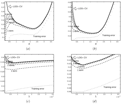
Figure 2: Comparison of training error (dotted line), approximations using (11) (dashed lines), the

proposed criterion C_IFk with k=5 (solid line), the exact leave-one-out error and the CV

approximation (both collapsing with C_IFk on these plots). Situation(a): as a function ofσ

atλ=0.001,(b)as a function ofσatλ=0.005,(c)as a function ofλatσ=1,(d)as a

function ofλatσ=2.

instance the influence function is almost 0. When we change z from[5,0.5]to[5,1], the influence

function changes too. It still has the same oscillating behavior, but the peaks are now higher. This reflects the non-robustness of the least squares estimator: if we would continue raising the point

z, then IF(z; f_λ,K)would become larger and larger, since it is an unbounded function of z. When

it comes down to model selection, it is interesting to check the effect of the hyperparameters in

play. When we change the bandwidthσfrom 1 to 2, the peaks in the resulting influence function in

Figure 1 are less sharp and less high. This reflects the loss in stability when small bandwidths are chosen: then the fit is more sensitive to small changes in the data and thus less stable.

Consider now the approximation of the leave-one-out error using the influence functions. We

still use the same data as in the previous paragraph. The dashed lines in Figure 2(a)show the

2 3 4 5 6 7 8 9 10 11 −1.5

−1 −0.5 0 0.5 1 1.5

X

Y

L=Huber

L=Least Squares

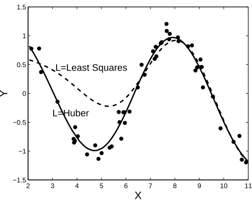
Figure 3: Data with outlier at(4,5). The parametersλ=0.001 andσ=2 are fixed. Dashed: KBR

with least squares loss function. Solid: KBR with Huber loss function (b=0.2).

λ=0.001 as a function of the bandwidthσ. We observe convergence from the training error towards

the leave-one-out error as the number of terms included is increased. Unfortunately the convergence

rate depends on the value ofσ: convergence is quite slow at small values ofσ. This is no surprise

looking at (12). There we approximated the remainder term by a quantity depending on(1₋Hi,i)−1.

Whenσis small, the diagonal elements of H become close to 1. In that case the deleted remainder

term can indeed be quite large. Nevertheless, this approach can still be useful if some care is taken

not to consider values ofλandσthat are too small. However, the criterion C_IF5 from Definition 8

us-ing the approximation in (12) is clearly superior. We see that the remainder term is now adequately

estimated and a good approximation is obtained at anyσ. The resulting curve is undistinguishable

from the exact leave-one-out error. The mean absolute difference is 3.2 10−5, the maximal

differ-ence is 1.8 10−4. The CV approximation also yields a good result being indistinguishable from

the exact leave-one-out error on the plot as well. The mean absolute difference is 4.1 10−4and the

maximal difference equals 1.8 10−3. Thus C_IF5 is closer to the true leave-one-out error than CV,

although the difference is irrelevant when it comes down to selecting a goodσ.

Figure 2 also shows plots for the leave-one-out error and its various approximations at (b)

λ=0.005 as a function ofσ,(c) σ=1 as a function ofλ,(d)σ=2 as a function ofλ. In these

cases as well it is observed that the cutoff strategy yields decent results if a sufficient number of

terms is taken into account and if one does not look at values ofλandσthat are extremely small.

The best strategy is to take the remainder term into account using the criterion C_IFk from Definition 8.

In Figure 3 we illustrate robustness. An (extreme) outlier was added at position (4,5) (not

visible on the plot). This outlier leads to a bad fit when LS-KBR is used withλ=0.001 andσ=2

(dashed line). When a Huber loss function is used with b=0.2 a better fit is obtained that still

1 1.5 2 2.5 3 3.5 1.34

1.36 1.38 1.4 1.42

σ

V Least Squares

C_IF5 LOO

1 1.5 2 2.5 3 0.35

0.36 0.37 0.38 0.39

σ V=L

1

C

IF 5

LOO

2 3 4 5 6 7 8 9 10 11 −1.5

−1 −0.5 0 0.5 1 1.5

X

Y

V = Least Squares

V=L 1

(a) (b)

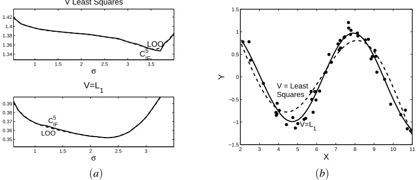
Figure 4: (a) Optimization of σ at λ=0.001. Upper: using least squares loss V in the model

selection. Lower: using L1 loss V in the model selection. For the estimation the loss

function L is always the Huber loss with b=0.2.(b)Resulting fits. Dashed line:σ=3.6

(optimal choice using V least squares). Solid line:σ=2.3 (optimal choice using L1loss

for V .

well. However, note that in this example as well as in Proposition 5 the hyperparametersλandσare

assumed to have fixed values. In practice one wants to choose these parameters in a data driven way.

Figure 4(a)shows the optimization ofσatλ=0.001 for KBR with L the Huber loss with b=0.2.

In the upper panel the least squares loss is used for V in the model selection criteria. Both exact

leave-one-out and C_IF5 indicate that a value ofσ_≈3.6 should be optimal. This results in the dashed

fit in Figure 4(b). In the lower panel of Figure 4 the L1loss is used for V in the model selection

criteria. Both exact leave-one-out and C_IF5 indicate that a value ofσ_≈2.3 should be optimal. This

results in the solid fit in Figure 4(b). We clearly see that, although in both cases a robust estimation

procedure is used (Huber loss for L), the outlier can still be quite influential through the model selection. To obtain full protection against outliers, both the estimation and the model selection step require robustness, for example by selecting both L and V in a robust way.

Finally let us investigate the role of the parameter b used in the Huber loss function. We now

use C5_IF with V the L1 loss. When we apply C_IF5 to the clean data without the outlier, we observe

in Figure 5(a) that the choice of b does not play an important role. This is quite expected: since

there are no outliers, there is no reason why least squares (b=∞) would not perform well. On the

contrary, if we use a small b such as b=0.1 we get a slightly worse result. Again this is not a

surprise, since with small b we will downweight a lot of points that are actually perfectly ok.

The same plot for the data containing the outlier yields a different view in Figure 5(b). The

values of C_IF5 are much higher for least squares than for the Huber loss with smaller b. Thus it

is automatically detected that a least squares loss is not the appropriate choice, which is a correct assessment since the outlier will have a large effect (cf. the dashed line in Figure 3). The criterion

1 1.5 2 2.5 3 0.1

0.11 0.12 0.13 0.14 0.15 0.16 0.17 0.18 0.19 0.2

σ

C IF

5 _b=0.1

b=0.2

b=1≈ b=∞

1 1.5 2 2.5 3 0.35

0.4 0.45 0.5 0.55 0.6

σ

C IF

5

b=∞

b=1

b=0.2 b=0.1

(a) (b)

Figure 5: C_IF5 atλ=0.001 as a function ofσfor several values of b for(a)the clean data without

the outlier,(b)the data with the outlier.

6.2 Other Examples

This part presents the results of a small simulation study. We consider some well known settings.

• Friedman 1 (d =10): y(x) =10 sin(πx1x2) +20(x3−1/2)2+10x4+5x5+∑10i=60.xi. The

covariates are generated uniformly in the hypercube inR10_.

• Friedman 2 (d=4): y(x) =₃₀₀₀1 (x2₁+(x2x3₋(x2x4)−2₎₎1/2_{, with 0<x1<100, 20<x2/(2π)<}

280, 0<x3<1, 1<x4<11.

• Friedman 3 (d=4): y(x) =tan−1(x2x3−(x2x4)−2

x1 ), with the same range for the covariates as

in Friedman 2. For each of the Friedman data sets 100 observations were generated with Gaussian noise and 200 noise free test data were generated.

• Boston Housing Data from the UCI machine learning depository with 506 instances and 13

covariates. Each split 450 observations were used for training and the remaining 56 for test-ing.

• Ozone data from ftp://ftp.stat.berkeley.edu/pub/users/breiman/ with 202 instances and 12

co-variates. Each split 150 observations were used for training and the remaining 52 for testing.

• Servo data from the UCI machine learning depository with 167 instances and 4 covariates.

Each split 140 observations were used for training and the remaining 27 for testing.

For the real data sets (Boston, Ozone and Servo), new contaminated data set were constructed as well by adding large noise to 10 training points, making these 10 points outliers.

The hyperparametersλandσare optimized over the following grid of hyperparametervalues:

• For each data set 500 distances were calculated between two randomly chosen observations.

Let d(i)be the ith largest distance. Then the following grid of values forσis considered:

σ∈ {1

2d(1),d(1),d(50),d(100),d(150),d(200),d(250),d(300),d(350),d(400),d(450),d(500),2d(500)}.

In each replicate the Mean Squared Error of the test data is computed. For every data set the average MSE over 20 replicates is shown in Table 1 (upper table). A two-sided paired Wilcoxon rank test is used to check statistical significance: values in italic are significantly different from the smallest

value at significance level 0.05. If underlined significance holds even at significance level 10−4.

Standard errors are shown as well (lower table). First we consider the least squares loss for L with

the criterion C_IF5 (λ,σ,∞)(Definition 8), with exact leave-one-out (17) and with CV (22). These are

the first 3 columns in Table 1. We see that the difference between these 3 criteria is very small. This

means that both CV and C5

IF provide good approximations of the leave-one-out error.

Secondly, we considered each time the residuals of the least squares fit with optimal λ and

σ according to C_IF5 (λ,K,∞). An estimate ˆσerr of the scale of the residuals is computed as the

MAD of these residuals (18). Then we applied KBR with a Huber loss and parameter b=3 ˆσerr.

The resulting MSE with this loss andλandσminimizing C_IF5 (λ,σ,3 ˆσerr)is given in column 4 in

Table 1. Similar results are obtained for b=2 ˆσerr in column 5 and with b=σˆerr in column 6. For

the data sets without contamination we see that using a Huber loss instead of least squares gives similar results except for the Boston housing data, Friedman 1 and especially Friedman 2. For those data sets a small value of b is inappropriate. This might be explained by the relationship between the loss function and the error distribution. For a Gaussian error distribution least squares is often an optimal choice (cf. maximum likelihood theory). Since the errors in the Friedman data are explicitly generated as Gaussian, this might explain why least squares outperforms the Huber loss. For real data sets, the errors might not be exactly Gaussian, and thus other loss function can perform at least equally well as least squares. For the data sets containing the outliers the situation changes of course. Now least squares is not a good option because of its lack of robustness. Clearly the outliers have a large and bad effect on the quality of the predictions. This is not the case when the Huber

loss function is chosen. Then the effect of the outliers is reduced. Choosing b=3 ˆσerralready leads

to a large improvement. Decreasing b leads to even better results (note that the p-values are smaller

than 10−4for any significant pairwise comparison).

Finally we also consider optimizing b. We apply the algorithm outlined in Section 5.2. Corre-sponding MSE’s are given in the last column of Table 1. For the Friedman 1 and Friedman 2 data sets for instance this procedure indeed detects that least squares is an appropriate loss function and automatically avoids choosing b too small. For the contaminated data sets the procedure detects that least squares is not appropriate and that changing to a Huber loss with a small b is beneficial, which is indeed a correct choice yielding smaller MSE’s. In fact, only for the Friedman 2 data, the automatic choice of b is significantly worse than the optimal choice (p-value=0.03), whereas the

benefits at the contaminated data are large (all p-values<10−4).

7. Conclusion

esti-b=∞(=LS) b=3 ˆσerr b=2 ˆσerr b=σˆerr (b=optimized)

LOO CV C5_IF C_IF5 C_IF5 C_IF5 C_IF5

F1 1.63 1.63 1.63 1.66 1.70 1.82 1.67

F2 1.30 1.30 1.30 1.42 1.71 3.02 1.39

F3 2.42 2.42 2.42 2.42 2.42 2.37 2.38

B 10.58 10.58 10.58 10.82 11.30 12.21 10.79

O 13.91 13.92 13.91 13.76 13.73 13.91 13.94

S 0.40 0.40 0.40 0.43 0.41 0.41 0.40

B+o 37.54 37.54 37.54 14.60 13.73 12.68 12.78

O+o 78.78 78.78 78.77 21.20 18.85 16.74 16.74

S+o 1.60 1.60 1.60 0.61 0.54 0.46 0.46

b=∞(=LS) b=3 ˆσerr b=2 ˆσerr b=σˆerr (b=optimized)

LOO CV C_IF5 C_IF5 C_IF5 C_IF5 C_IF5

F1 0.09 0.09 0.09 0.09 0.10 0.08 0.09

F2 0.14 0.14 0.15 0.16 0.20 0.36 0.15

F3 0.03 0.03 0.03 0.03 0.03 0.05 0.05

B 1.39 1.39 1.39 1.40 1.46 1.51 1.39

O 0.86 0.86 0.87 0.78 0.78 0.75 0.81

S 0.05 0.05 0.05 0.09 0.08 0.09 0.09

B+o 2.91 2.91 2.91 1.12 1.09 1.02 1.04

O+o 3.44 3.44 3.44 1.01 0.97 1.03 1.03

S+o 0.16 0.16 0.16 0.07 0.07 0.08 0.08

Table 1: Simulation results. Upper: Mean Squared Errors. Lower: standard errors. Friedman 1 (F1), Friedman 2 (F2), Friedman 3 (F3), Boston Housing (B), Ozone (O), Servo (S), Boston Housing with outliers (B+o), Ozone with outliers (O+o) and Servo with outliers (S+o). Italic values are significantly different from the smallest value in the row with

p-value in between 0.05 and 0.001 using a paired Wilcoxon rank test; underlined values are

significant with p-value<10−4.

mator. Experiments indicate that the quality of this approximation is quite good. The approximation is used in a model selection criterion to select the regularization and kernel parameters.

We discussed the importance of robustness in the model selection step. A specific procedure

is suggested using an L1 loss in the model selection criterion and a Huber loss in the estimation.

Acknowledgments

JS acknowledges support from K.U. Leuven, GOA-Ambiorics, CoE EF/05/006, FWO G.0499.04, FWO G.0211.05, FWO G.0302.07, IUAP P5/22.

MH acknowledges support from FWO G.0499.04, the GOA/07/04-project of the Research Fund KULeuven, and the IAP research network nr. P6/03 of the Federal Science Policy, Belgium.

Appendix A.

Proof of Theorem 6

Let P be a distribution, z_∈

X

Y

We start from the representer theorem of DeVito et al. (2004) (a generalization of (13)):

2λf_λ,K,Pε,z =EPε,z[L0(Y−fλ,K,Pε,z(X))Φ(X)].

By definition of P_ε,zand sinceE∆zg(X) =g(z)for any function g:

2λf_λ,K,Pε,z= (1−ε)EP[L

0_(Y−f

λ,K,Pε,z(X))Φ(X)] +εL

0_(z

y−fλ,K,Pε,z(zx))Φ(zx).

Taking the first derivative on both sides with respect toεyields

2λ_∂ε∂ f_λ,K,Pε,z=(1−ε)EP[−

∂

∂εfλ,K,Pε,z(X)L

00_(Y−f

λ,K,Pε,z(X))Φ(X)]

−E_P[L0_(Y−fλ,K,P

ε,z(X))Φ(X)] +L0(zy−fλ,K,Pε,z(zx))Φ(zx)

−ε_∂ε∂ f_λ,K,Pε,z(zx))L00(zy−fλ,K,Pε,z(zx))Φ(zx).

The second derivative equals

2λ ∂

∂2εfλ,K,Pε,z=−EP[−

∂

∂εfλ,K,Pε,z(X)L

00_(Y−f

λ,K,Pε,z(X))Φ(X)]

+ (1₋ε)E_P[− ∂

∂2εfλ,K,Pε,z(X)L

00_(Y−f

λ,K,Pε,z(X))Φ(X)]

+ (1−ε)E_P[₋∂

∂εfλ,K,Pε,z(X)L

000_(Y−f

λ,K,Pε,z(X))(−

∂

∂εfλ,K,Pε,z(X))Φ(X)]

−E_P[L00_(Y−fλ,K,P

ε,z(X))(−

∂

∂εfλ,K,Pε,z(X))Φ(X)]

−_∂ε∂ f_λ,K,Pε,z(zx)L00(zy−fλ,K,Pε,z(zx))Φ(zx)

−ε_∂∂2εfλ,K,Pε,z(zx)L

00_(z

y−fλ,K,Pε,z(zx))Φ(zx)

−ε_∂ε∂ f_λ,K,Pε,z(zx)L

000_(z

y−fλ,K,Pε,z(zx))(−

∂

∂εfλ,K,Pε,z(zx))Φ(zx)

−L00(zy−fλ,K,Pε,z(zx))

∂