Joint Structural Estimation of Multiple Graphical Models
Jing Ma [email protected]
Department of Biostatistics and Epidemiology Perelman School of Medicine
University of Pennsylvania
211 Blockley Hall, 423 Guardian Drive Philadelphia, PA 19104, USA
George Michailidis [email protected]
Department of Statistics University of Florida
205 Griffin-Floyd Hall, P.O. Box 118545 Gainesville, FL 32611, USA
Editor:Nicolai Meinshausen
Abstract
Gaussian graphical models capture dependence relationships between random variables through the pattern of nonzero elements in the corresponding inverse covariance matrices. To date, there has been a large body of literature on both computational methods and analytical results on the estimation of asinglegraphical model. However, in many application domains, one has to estimate severalrelatedgraphical models, a problem that has also received attention in the literature. The available approaches usually assume that all graphical models aregloballyrelated. On the other hand, in many settings different relationships between subsets of the node sets exist between differ-ent graphical models. We develop methodology thatjointlyestimates multiple Gaussian graphical models, assuming that there exists prior information on how they are structurally related. For many applications, such information is available from external data sources. The proposed method con-sists of first applying neighborhood selection with a group lasso penalty to obtain edge sets of the graphs, and a maximum likelihood refit for estimating the nonzero entries in the inverse covariance matrices. We establish consistency of the proposed method for sparse high-dimensional Gaussian graphical models and examine its performance using simulation experiments. Applications to a climate data set and a breast cancer data set are also discussed.
Keywords: Gaussian graphical model, structured sparsity, group lasso penalty, consistency, edge set recovery
1. Introduction
There has been a large amount of work over the last few years on estimating Gaussian graphical models from high-dimensional data. In this family of models, jointly normally distributed random variables are represented by the nodes of a graph, while its edges reflect conditional dependence relationships amongst nodes that are captured through the nonzero entries of the inverse covariance matrix (or precision matrix) (Lauritzen, 1996; Edwards, 2000). Formally, letXbe ap-dimensional multivariate normal random vector where
For 1 ≤ i 6= j ≤ p,Xi andXj are said to be conditionally independent given all the remaining
variables, if the corresponding entry in the precision matrixΩ = Σ−1 is zero. An edge between the nodesXi andXj in the graph implies that they are conditionally dependent and corresponds
to a nonzero entry in the precision matrix. To identify the graph, one only needs to select the corresponding precision matrix.
B¨uhlmann and van de Geer (2011, chap. 13) gave an overview of statistical methods developed for estimating a Gaussian graphical model subject to sparsity constraints, an attractive feature that reduces the number of parameters to be estimated and also enhances interpretability of the results. These models have found applications in diverse fields including analysis of omics data (Perroud et al., 2006; Pujana et al., 2007; Putluri et al., 2011), reconstruction of gene regulatory networks (Dehmer and Emmert-Streib, 2008, chap. 6), as well as study of climate networks (Zerenner et al., 2014).
More recently, the focus has shifted from estimating a single graphical model to joint estimation of multiple graphs due to the availability of heterogeneous data (see discussion in Guo et al., 2011). For example, climate models capturing relationships between climate defining variables over a large area share common patterns; i.e. there areshared common linksand also sharing ofabsence of links
between the models (networks at different spatial locations). While separate estimation of indi-vidual models without taking the known pattern into consideration ignores the common structure, estimating one single model could mask the differences that could prove critical in understanding local climate features.
Several authors have studied the problem ofjointlyestimating multiple graphical models under different assumptions on how the models are related. Guo et al. (2011) introduced a procedure us-ing a hierarchical penalty on the log-likelihood, whose objective is to estimate the common zeros (absence of edges) in the precision matrix across all graphical models under consideration. Thus, the procedure borrows strength across models through the the non-connected nodes, but does not impose any structure on the connected ones. Danaher et al. (2014) proposed a joint graphical lasso by maximizing the log-likelihood subject to a generalized fused lasso or group lasso penalty, which can be solved efficiently by a standard alternating directions method of multipliers algorithm (Boyd et al., 2011). When employing a group lasso penalty, the underlying assumption is that the vari-ous observed graphical models are perturbationsof a single common connectivity pattern across all graphical models, while when using a fused lasso across all models a similar outcome occurs, although more heterogeneity between estimated graphical models can be obtained depending on the tuning of the penalties. The work by Zhu et al. (2014) investigates the joint estimation problem by introducing a truncated`1penalty on the pairwise differences between the precision matrices to
achieve entry-wise clustering of the network structure over multiple graphs. Peterson et al. (2015) introduced a Bayesian approach that links the estimation of the graphs via a Markov random field prior for common structures. Further, a spike-and-slab prior is placed on the parameters that mea-sure the similarity between graphs, thus relaxing the assumption on sharing a common structure across all graphical models.
the-oretical guarantees are provided for more general settings. Finally, many papers only present algo-rithms for joint estimation of the Gaussian graphical models under consideration, but no theoretical properties of the estimates (Honorio and Samaras, 2010; Chiquet et al., 2011; Danaher et al., 2014; Mohan et al., 2014).
In this paper, we investigate estimation of multiple graphical models undercomplex structural relationships, assuming that there existsprior informationon their specification. In many applica-tions, such information is available and may come from prior knowledge in the literature of relation-ships among different node subsets of the graphical models under consideration, or from clustering of all graphs. The approach allows sharing common sub-graph components between different mod-els and does not require sharing of values for the same element across multiple precision matrices. The proposed method, called theJointStructuralEstimationMethod(JSEM), leverages structured sparsity patterns as illustrated in Section 2 and is a two-step procedure. In the first step, we infer the sparse graphical models by incorporating the available structure through a group lasso penalty. In the second step, we maximize the Gaussian log-likelihood subject to the edge set constraints obtained from the previous step. Numerically, JSEM demonstrates superior performance in con-trolling both the number of false positive and false negative edges compared to available methods. When applied to joint modeling of climate networks, our results highlight the different roles climate defining factors play at different regions of the United States. In another application to breast can-cer gene expression data, the JSEM methodology reveals interesting differences in the molecular network rewiring between the ER+ and ER- classes (see extensive discussion in Section 5.2). Un-derstanding the rewiring of biological networks under different conditions provides deeper insights into biological mechanisms of disease, especially when combined with topology-based pathway enrichment methods as discussed and illustrated in Ma et al. (2016) and Kaushik et al. (2016).
The contributions of this work are three-fold. First, we develop a general framework for the problem of joint estimation of multiple Gaussian graphical models. The method can incorporate de-tailed structural information regarding relationships between subsets of the graphical models, while in the absence of such information reduces to the group graphical lasso procedure of Danaher et al. (2014). Further, we establish that the JSEM estimator is consistent with a fast rate of convergence in terms of the Frobenius norm for the estimated precision matrices. We also establish rigorously the consistent recovery of the edge sets for JSEM under suitable regularity conditions. Finally, when the externally provided structured sparsity pattern is moderately misspecified, we provide a mod-ified estimator that reduces the number of false positive edges identmod-ified due to prior information misspecification, thus further enhancing the applicability of JSEM.
The paper is organized as follows. Section 2 discusses the structural relationships model used in this work and presents the estimation procedure. Section 3 presents the theoretical properties of the proposed method, followed by simulation studies in Section 4 and two real data applications— climate modeling and genomics of breast cancer—are presented in Section 5. We conclude with a discussion in Section 6. Most details of the theoretical analysis and proofs, additional simulation results as well as additional analyses on the applications are relegated to the Appendix.
2. The Joint Structural Estimation Method
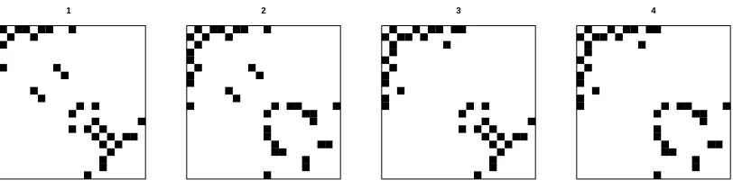
1 2 3 4
Figure 1: Image plots of the adjacency matrices for four graphical models with vertex set {1, . . . , p}. The black color represents presence of an edge. The structured sparsity pattern is encoded in G = ∪1≤i<j≤pGij, where Gij = {[1,3],[2,4]} for (i, j) ∈
{bp/2c+ 1, . . . , p}andGij ={[1,2],[3,4]}for all other pairs of(i, j).
row represents one observation fromN(0,Σk0), k = 1, . . . , K. Throughout the remaining sections, we reserve the notationsΣ0,Ω0, . . .to denote the population parameters in the true model and use
Σ,Ω, . . .to denote generic parameters. Without loss of generality, we assume the columns ofXk
are centered and standardized to have mean zero and unit variance. For ease of presentation, it is assumed that the sample sizenk =nfor allk= 1, . . . , K, but the modeling framework can easily
accommodate unequal sample sizes. Our goal is to estimate jointlyΩk0 = (Σk0)−1 for allk, under the assumption that theKcorresponding graphs are related via a structured sparsity patternG. For example, consider climate models capturing relationships between climate forcing variables defined over a pre-specified spatial domain. Models that belong to the same climate zone may exhibit greater similarity in their graph structures than those from different zones. Thus, one can defineG based on their spatial locations. Figure 1 gives an illustration of the structured sparsity among four graphical models in terms of their adjacency matrices. This pattern indicates that sharing of structures may occur at different subsets of the edge set, which motivates us to develop a joint estimation method that can incorporate such rich and complex structural information.
2.1 Neighborhood Selection
Neighborhood selection was introduced by Meinshausen and B¨uhlmann (2006) as an efficient method to construct Gaussian graphical models from high-dimensional data. For each nodei= 1, . . . , pin the graphical model, consider the optimal prediction of the random variableXi as a linear
combi-nation of the remaining variables:
Xi =
X
j6=i
θijXj+εi,
whereθij (j 6= i)are the regression coefficients andεi ⊥ {Xj : j 6= i}. The matrix(θij)1≤i,j≤p
is determined by the inverse covariance matrixΩ = (ωij)1≤i,j≤p. Specifically, it holds thatθij =
−ωij/ωii,for allj 6= i. The set of nonzero coefficients ofθij (j 6= i) is thus the same as the set
of nonzero entries in the row vector of ωij (j 6= i), which defines the set of neighbors of nodei.
Using anl1-penalized regression, Meinshausen and B¨uhlmann (2006) estimated the neighborhood
2.2 An Illustrative Example
We first illustrate how to extend the idea of neighborhood selection to multiple graphical models us-ing the example in Figure 1. Fork= 1, . . . , K, let(θkij)p×pbe the matrix of regression coefficients
in graphkandθki the vector of allθijk (j 6=i)for nodei= 1, . . . , p. Unless otherwise stated, all vectors are assumed to be column vectors. For nodeiin a single graphk, neighborhood selection suggests estimating the coefficientsθki by
min
θki
1
nkX
k
i −Xk−iθkik2+ 2λ
X
j6=i
|θijk|,
whereXk
−iisXkwith thei-th column removed,k · krepresents the standard Euclidean norm and
λis the regularization parameter. To achieve joint estimation, consider the following regularized regression problem
min
Θi
1
n
K
X
k=1
kXki −Xk−iθikk2+ 2Pλ(Θi), (1)
whereK = 4,Θi = (θ1i, . . . ,θKi )andPλ(Θi)is a regularization term to be determined next. Note that each column ofΘi represents the regression coefficients from one graphical model and each row ofΘicorresponds to the four coefficients at the same(i, j)pair.
The penalty Pλ(Θi) is chosen based on information from the structured sparsity patternG in Figure 1. For example, fori= 1with grouping{[1,2],[3,4]},
Θ1=
θ121 θ212 θ312 θ124 ..
. ...
θ11p θ21p θ31p θ14p
.
As indicated by the colors, we can then group the coefficients in thej-th row ofΘ1(j= 2, . . . , p)
as
(θ11j, θ12j | {z } θ[11j,2]
, θ13j, θ14j | {z } θ[31j,4]
)
and setPλ(Θ1)to be the group lasso penalty
X
j=2,...,p
X
g=[1,2],[3,4]
λg1jkθ[1gj]k.
The group lasso penalty forces the two coefficients in each group to be zero or nonzero at the same time, leading to the same structure for graphical models belonging to the same group.
The solutionΘiˆ to (1) fori= 1, . . . , pcan then be used for graph selection.
2.3 The General Case
Denote the structured sparsity pattern byG =∪1≤i<j≤pGij, where the union is over allp(p−1)/2
knowledge on the structural similarity for the(i, j)-th pair across models. For example in Figure 1,Gij = {[1,2],[3,4]}means that the graphs 1 and 2 exhibit the same structure at(i, j), whereas 3 and 4 behave the same at(i, j). It is possible for all four graphs to have the edge(i, j) or not have the edge (i, j) at the same time, but we do not impose this restriction. Taking the union over all pairs,G ={[1,2],[3,4],[1,3],[2,4]}in Figure 1. Therefore the patternG allows a more flexible structural relationships among multiple graphical models. Further, the sparsity pattern inG is symmetric as we requireGji =Gij fori < j.
For1≤i < j ≤pand a groupg∈Gij, denote byθ[g]
ij the vector(θkij)k∈g, a concatenation of all
regression coefficients from graphs ing. The grouping for the regression coefficients(θ1ij, . . . , θKij)
is determined byGij. Under correctly specifiedG, all coefficients in the same group should be zero or nonzero simultaneously. Fork = 1, . . . , K, letEk ={(i, j) : θijk 6= 0}be the set of undirected edges in graphkandS+
Ek ={Ω : Ω0andωij = 0for all(i, j)∈/ Ekwherei6=j}.
TheJoint Structural Estimation Method(JSEM) proceeds with the following two steps.
(I) Fork= 1, . . . , K, we infer the sparse graphsEˆkthrough the following group lasso estimator. Fori= 1, . . . , p,
min
Θi
1
n
K
X
k=1
kXki −Xk−iθkik2+ 2
X
j:j6=i
X
g∈Gij
λgijkθ[ijg]k
. (2)
ˆ
Ekis estimated to be the set
{(i, j) : 1≤i < j ≤p,θˆkij 6= 0ORθˆkji6= 0}. (3)
(II) We refit the model by
min
Ωk∈S+
ˆ
Ek
n
tr( ˆΣkΩk)−log det(Ωk)o, k= 1, . . . , K. (4)
Note the grouped variables in (2) are non-overlapping becauseGij partitions the set{1, . . . , K} into disjoint subsets. The ‘OR’ rule defined in (3) can be replaced by the ‘AND’ rule. The problems in (2) and (4) are both convex and can thus be solved by available convex optimization algorithms. In this work, we use the R-package grpreg(Breheny and Huang, 2009) for implementation of the group lasso penalized optimization (2) and theglasso(Friedman et al., 2008) one for solv-ing (4). The computational complexity for step (II) isO(Kp3) using the standard graphical lasso algorithm. Sincegrpreguses a coordinate descent algorithm, the computational complexity for step (I) can be as fast asO(nKp2)if the number of graphsK does not exceed the sample sizen,
orO(K2p2)otherwise. Thus, the overall computational complexity of JSEM isO(Kp3)ifp > K, andO(K2p2)otherwise.
2.4 Choice of Tuning Parameters
based on the latter approach. We recommend choosing the tuning parameters via the Bayesian information criterion (BIC). Specifically, for a givenλ, we defineBICfor the proposed method as
BIC(λ) =
K
X
k=1
tr( ˆΣkΩˆkλ)−log det( ˆΩkλ) +log(nk)
nk
|Eˆk|
,
whereΩˆkλ(k = 1, . . . , K)are the estimated precision matrices from the data. The optimal tuning parameter is thus λ∗ = argminλ∈DnBIC(λ), where the set of values Dn is chosen such that for
everyλj ∈ Dn(nk=n):
λj =cj
|gmax|+
p
logG0
√
n, cj = 0.02∗j, j= 1, . . . ,20.
Here|gmax|andG0 refer, respectively, to the maximum size of groups inG and maximum total
number of groups in all regressions. They can be conveniently defined by the input sparsity pattern. In practice, it is also recommended to apply the stability selection procedure (Meinshausen and B¨uhlmann, 2010; Shah and Samworth, 2013) to select graphical models that are both stable and interpretable.
3. Theoretical Results
The JSEM estimator enjoys nice theoretical properties under certain regularity conditions. Specifi-cally, we establish the norm consistency of the estimated precision matrices, as well as the consistent recovery of the edge sets of the various graphical models under consideration based on the structured sparsity patternG.
3.1 Estimation Consistency
LetNi(p−1)K ={(j, k) :j6=i, k= 1, . . . , K}be the variable index set for equation (2) with a fixed
nodei. Given the structural informationG, the grouped variable index set{(j, g) :j6=i, g∈Gij}
defines a partition ofNi(p−1)K. Denote by Gi the cardinality of the set{(j, g) : j 6= i, g ∈ G ij}.
Then1≤Gi≤(p−1)K. LetJ(Θ0,i) ={(j, g) :j=6 i, g∈Gij,θ0[g,ij] 6= 0}be the set of nonzero
groups in thei-th regression. We assume an overall sparsity at the group level, that is, the size of J(Θ0,i)issi<< Gi. Let
G0 = max
i=1,...,pGi, s0= maxi=1,...,psi, S0 = p
X
i=1
si,
and also let|g|be the size of the groupgwith|gmax|= maxg∈G|g|.
LetM(p, K)represent the set of allp×K matrices. For∆ = (δ1, . . . ,δK) ∈ M(p, K)and
a group g ⊂ {1, . . . , K}, denote byδj[g] the vector composed of all δjk for whichk ∈ g. Write J ={J(Θ0,1), . . . , J(Θ0,p)}, the collection of sets of nonzero groups in allpregressions. For any
J ∈ J, denote∆J the nonzero matrix inM(p, K), which has the same coordinates as∆onJ and
zero elsewhere. LetJc denote the complement of the index setJ. Write0 as the zero matrix in
(A1) For0< s < G0, there existsκ=κ(s)>0, such that
min
J∈J,|J|≤s∆∈FminJ
PK
k=1kXkδkk2/n
k∆Jk2F
≥κ2(s),
where forisatisfyingJ(Θ0,i) =J,FJ is defined as
FJ ={∆ : ∆∈M(p, K)\{0}, X
(j,g)∈Jc
λgijkδ[jg]k ≤3 X
(j,g)∈J
λgijkδ[jg]k}.
(A2) For everyk= 1, . . . , K andi= 1, . . . , p,Var(Xik) = 1. Further, there exist constantsc0and
d0 such that for everyk,
0<1/c0 ≤φmin(Σk0)≤φmax(Σk0)≤1/d0 <∞,
whereφmin(Σk0) andφmax(Σk0) are the minimum and maximum eigenvalues of the matrix
Σk0, respectively.
Assumption (A1) is a generalization of the Restricted Eigenvalue assumption for the Lasso in Bickel et al. (2009) to the group lasso setting in our problem and requires the super design matrix
diag(X1, . . . ,XK) to be well conditioned over the restricted set of vectors under consideration. One sufficient condition is that the eigenvalues of the Gram matrix ofdiag(X1, . . . ,XK)is positive when restricted to the subset of sparse vectors with cardinality no greater than2s.
The equal variance requirement in assumption (A2) can be easily achieved by appropriate scal-ing of the data. The second part of the assumption explicitly excludes sscal-ingular or nearly sscal-ingular covariance matrices and guarantees thatΩk0 exists for every modelk= 1, . . . , K.
We are now ready to state our first result.
Theorem 1 ConsiderΩˆk (k = 1, . . . , K) defined in(4). Let Assumption (A1) withs = 2s0 and
Assumption (A2) be satisfied. For every regression defined in(2), choose
λgij = √2 nd0
p
|gmax|+
π √
2
p
qlogG0
,
withq >1. Then, with probability at least1−2pG1−0 q, we have 1
K
K
X
k=1
kΩˆk−Ωk0kF ≤O r
S0
nK
p
|gmax|+
π √
2
p
qlogG0
!
, (5)
whereG0 is the maximum number of groups in all regressions,S0 is the total number of relevant
groups and|gmax|is the maximum group size.
For example, if allKgraphs share the same structure, then|gmax|=K andG0 =p−1. Thus,
JSEM achieves a convergence rate of the order of
O r
S0
n (
1 +√π
2
r
qlog(p−1)
K
)!
. (6)
In contrast, separate estimation ofΩkis known to be of the order of
O s
X
k
kΩk,0−k0logp nK
!
,
where kΩk,0−k0 denotes the number of nonzero off-diagonal entries inΩk0 and P
k is short-hand
notation forPK
k=1. The joint estimation method by Guo et al. (2011) has the following convergence
rate
O r
(p+m)logp
nK !
,
where m = | ∪ {k = 1, . . . , K : ω0k,ij 6= 0}|. Under correctly specified G, we haveS0 = m.
Thus, JSEM has a lower estimation error rate than the joint estimation method of Guo et al. (2011). JSEM also outperforms separate estimation ifS0 kΩk,0−k0, wheremeans that the expressions
on both sides are of the same order. On the other hand, the rate in (6) could be worse if the sparsity patternG is highly misspecified such that the number of nonzero parametersS0 >PkkΩ
k,−
0 k0 ≥
m. The issue of sparsity pattern misspecification is addressed in the next section.
3.2 Graph Selection Consistency
To understand how JSEM performs in selecting the edge sets of the graphical models, it suffices to focus on each of the group lasso estimation problems (2), as consistent graph selection relies on con-sistent variable selection in allpregressions. Unlike the sign consistency in the lasso setting (Zhao and Yu, 2006), variable selection properties with a group lasso penalty are much more complicated because the latter selects whole groups rather than individual variables (see Basu et al., 2015, and the discussion therein). The Basu et al. (2015) paper offers a generalization and introduces the no-tion of direcno-tion consistency for the group lasso. Specifically, for a nonzero vectorξ, its direction vector is defined asD(ξ) =ξ/kξkandD(0) =0. An estimatorΘiˆ of (2) isdirection consistentat rateαnif for a sequence of positive real numbersαn→0,
P(kD(ˆθ
[g]
ij)−D(θ
[g]
0,ij)k< αn, ∀(j, g)∈J(Θ0,i); ˆθ
[g]
ij =0, ∀(j, g)∈/J(Θ0,i))→1,
asn, p→ ∞. In general, direction consistency does not guarantee sign consistency, especially when there are multiple members within one group. However, if the group is selected, all the members within the group are selected, which is sufficient for joint neighborhood selection for each node and subsequent selection of graphs. Motivated by the above idea, we establish the graph selection consistency property of JSEM in Theorem 2, which can be conveniently modified to adjust for the misspecification in the prior informationG. Before we present the main result, we need more notations.
denoteXkI
kthen× |Ik|sub-matrix consisting of all relevant variables from thek-th model. In other
words, for allj ∈Ik, there exists a groupg3ksuch that(j, g)∈J(Θ0,i). Note the dependency of
each index setIkoniis made implicit here for notational convenience. Further, letξk ∈ R|Ik|be
a vector indexed byIk. The following assumption adapts theUniform Irrepresentability Condition (IC)in Basu et al. (2015) to our setting:
(A3) There exists a positive constantηsuch that for allξ= ((ξ1)T, . . . ,(ξK)T)T ∈R
P
k|Ik|with
max
(j,g)
kξ[jg]k ≤1and all(j, g)∈/J(Θ0,i),
X
k∈g
h
(Xkj)TXkIk(XkIk)TXkIk −1ξk
i2
1/2
≤1−η. (7)
Note the group level constraint (7) is required to hold for allpregressions and is less stringent than the IC for the selection consistency of lasso. In general, it is not easy to verify Assumption (A3). One sufficient condition, as suggested in Zhao and Yu (2006), is that the regression coefficients of
Xkj onXkI
k (k= 1, . . . , K)have Euclidean norm less than 1 for all(j, g)∈/ J(Θ0,i).
Theorem 2 Let Assumption (A1) withs=s0, (A2) and (A3) be satisfied. Assume further that the
sparsity patternG is correctly specified. For every regression defined in(2), choose
λ≥ max
i,(j,g)∈/J(Θ0,i)
1
η
1
√ nd0
p
|g|+ √π
2
p
qlogG0
, (8)
αn≥ max i,(j,g)∈J(Θ0,i)
1
κ(s0)
1
kθ[0g,ij] k
λ √
s0
κ(s0)
+√1 nd0
p
|g|+√π
2
p
qlogG0
, (9)
withq >1. Then with probability at least1−4pG1−0 q, we have simultaneously for alli
1. θˆ[ijg]=0, for all(j, g)∈/ J(Θ0,i),
2. kθˆ[ijg]−θ[0g,ij] k< αnkθ[0g,ij] k, and hencekD(ˆθ
[g]
ij )−D(θ
[g]
0,ij)k<2αnfor all(j, g)∈J(Θ0,i). Further, ifαn<1, then
P( ˆEk =E0k,∀k= 1, . . . , K)≥1−4pG
1−q
0 .
whereEˆkis defined in(3).
Note the choice ofλin (8) is of the same order as the tuning parameter required for estimation consistency in Theorem 1. With the above choice of λ, αn can be chosen to be of the order of
O(√s0(
p
|gmax|+
√
logG0)/
√
n). A proof of Theorem 2 can be found in Appendix B.
Bach (2008) using a strong irrepresentability assumption also establishes group support recov-ery. In this work, we take a different route, where a similar strong irrepresentability assumption leads to direction consistency. Then, we leverage the notion of direction consistency to propose
that thesign(·)function in standard lasso KKT conditions is replaced by theD(·) function in the group lasso KKT conditions. Therefore, sign consistency has a natural generalized counterpart when considering optimization over groups.
When G is misspecified, it is possible that not all the members within a group have nonzero effects. However, the group lasso penalty may fail to exclude members with actual zero effect within the misspecified group, leading to the recovery of spurious edges. The following result implies that the property of direction consistency helps identify influential members within a group, that is, those with noticeable nonzero effects.
Corollary 3 Let Assumption (A1) with s = s0, (A2) and (A3) be satisfied. For every regression
defined in(2), chooseλandαnas in Theorem 2. Define
ˆ
θijk,thr= ˆθijk1{θˆkij/kθˆ[ijg]k>2αn}, ∀k∈g, ∀(j, g)∈J(Θ0,i),
and
ˆ
Ek,thr ={(i, j) : 1≤i < j ≤p,θˆijk,thr 6= 0 OR ˆθk,thrji 6= 0}.
If for allg∈G,min k∈g θ
k
0,ij/kθ
[g]
0,ijk>2αn, then
P( ˆEk,thr=E0k,∀k= 1, . . . , K)≥1−4pG
1−q
0 .
The result in Corollary 3 implies immediately that JSEM with an additional thresholding step on the estimated direction vectors D(kθˆ[ijg]k) can be applied to reduce false discoveries and thus improve selection of the edge sets when the structured patternG is moderately misspecified (that is, most of the structural relationships specified inG are reliable). This is illustrated in the third simulation study of Section 4.
4. Performance Evaluation
We present three simulation studies to evaluate the performance of JSEM. Other methods compared include the separate estimation method Glasso, where theGraphical lassoby Friedman et al. (2008) is applied to each graphical model separately, joint estimation by Guo et al. (2011), denoted by JEM-G, the Group Graphical Lasso denoted by GGL by Danaher et al. (2014), and the structural pursuit method MGGM by Zhu et al. (2014). Note we choose MGGM over the Fused Graphical Lasso method (Danaher et al., 2014), as the former has been consistently shown to exhibit better performance.
The third simulation compares JSEM with its thresholded version under misspecifiedG using the experimental settings of the first two studies. In this setting, one also needs to select the within group thresholdingαnbesidesλ. As in previous simulations, we first selectλviaBICwithout any
thresholding. At the optimalλ, we selectαnfrom the grid of values
αn(c) =c
|gmax|+
p
logG0
√
n, c∈ {0.1,0.2, . . . ,1},
where|gmax|andG0are defined by the input sparsity pattern. The optimalα∗nis selected as the one
that minimizes the correspondingBIC.
We refer readers to Appendix C for additional simulation results, including comparison of all joint estimation methods with and without maximum likelihood refitting step (4), and largep set-tings.
4.1 Simulation Study 1
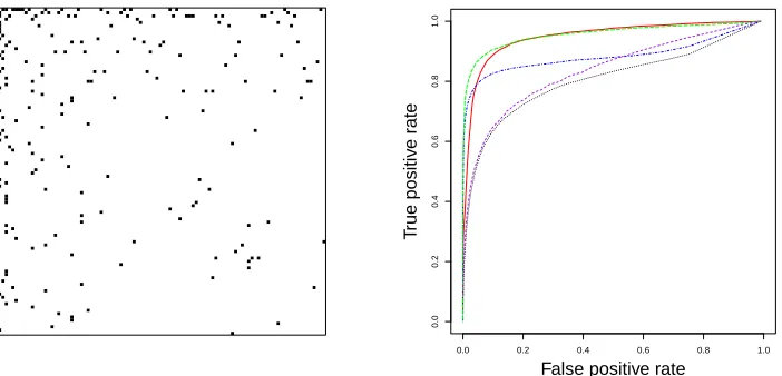
In our first simulation, we set K = 5, with each graphical model being of size p = 100. The structured pattern is constructed as follows: we first generate a scale-free network with edge setE0
as the common structure shared across all graphs, shown in the left panel of Figure 2. To generate the edge setEk, we randomly select a pair of(i, j), i < j such that(i, j) ∈/ E0 and add it toEk.
This procedure was repeatedρ|E0|times for eachk, where ρ is a positive number corresponding
to the ratio of individual edges to common ones. In this example, we set ρ = 0.1to allow high structural similarity across graphs. Thus, all graphical models have the same degree of sparsity, with 108 or 2.2% of all possible edges present. Note that due to the sparse structure of each graph, the proportion of shared non-edges (common zeros in the adjacency matrices) among all models is 98%.
Given the edge set Ek, we then constructed the inverse covariance matrix with the nonzero
off-diagonal entries inΩk being uniformly generated from the[−1,−0.5]∪[0.5,1]interval. The positive definiteness ofΩk is guaranteed by setting the diagonal elements to be|φmin(Ωk)|+ 0.1.
The covariance matrixΣkis then determined by Σkij = (Ωk)−1ij /
q
(Ωk)−1 ii (Ωk)
−1
jj .
By construction, eachΣkcorresponds to the correlation matrix for thek-th graphical model. The sparsity pattern supplied for JSEM isG ={1, . . . , K}, that is assuming all graphical models share the same structure. Note by setting the parameterρ= 0.1, we have created a situation where about 10% of the information in G is misspecified for JSEM. This is of interest for us to see whether JSEM is robust to pattern misspecification.
To compare the overall performance of all methods, we generatednk = 50samples from each
k = 1, . . . , K and computed the average false positive and true positive rates of the estimated precision matrices over a fine grid of tuning parameters from 20 replications. The resulting ROC curves are shown in the right panel of Figure 2. Since both GGL and MGGM require two tuning parameters, one for controlling the sparsityof individual graph and the other for controlling the
0.0 0.2 0.4 0.6 0.8 1.0
0.0
0.2
0.4
0.6
0.8
1.0
False positive rate
T
rue positiv
e r
ate
Figure 2: Simulation study 1: left panel shows the image plot of the adjacency matrix corresponding to the shared structure across all graphs. Each black cell indicates presence of an edge. The right panel shows the ROC curves for sample sizenk= 50: Glasso (dotted in black),
JEM-G (dotdash in blue), GGL (solid in red), MGGM (dashed in purple), JSEM (long-dash in green).
penalty. In this example, it turns out that GGL performs the best when there is only regularization on the similarity, i.e. agroup lassopenalty on the same entry across allKprecision matrices, which we expect to exhibit a similar performance to the proposed JSEM. In the right panel of Figure 2, the ROC curve of GGL falls slightly below that of JSEM. In comparison, MGGM does not perform as well despite the flexible penalty. The best curve we got from MGGM shows some advantage over the separate estimation Glasso, but mostly falls below curves from other joint estimation methods. JEM-G performs well and is very competitive compared to GGL and JSEM for very low false positive and high true positive rates, but starts falling behind when the false positive rate is greater than 5%. In this example, JSEM performs the best with the highest ROC curve throughout the domain.
Next, we computed the estimators from different methods with nk = 50 samples for each
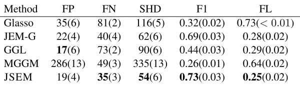
k = 1, . . . , K, using the tuning parameters selected byBIC. Results are summarized in Table 1, which compares the estimated precision matrices with the population version in the true model based on 50 replications under falsely discovered edges (FP), falsely deleted edges (FN), structural hamming distance (SHD),F1score (F1) and Frobenius norm loss (FL). TheF1score (based on the
Method FP FN SHD F1 FL Glasso 35(6) 81(2) 116(5) 0.32(0.02) 0.73(<0.01) JEM-G 22(4) 40(4) 62(6) 0.69(0.03) 0.28(0.02)
GGL 17(6) 73(2) 90(6) 0.44(0.03) 0.29(0.02)
MGGM 286(13) 49(3) 335(13) 0.26(0.01) 0.64(0.02) JSEM 19(4) 35(3) 54(6) 0.73(0.03) 0.25(0.02)
Table 1: Performance of different regularization methods for estimating graphical models in Simu-lation Study 1: average FP, FN, SHD, F1 and FL (SE) for sample sizenk = 50. The best
cases are highlighted in bold.
a balance and obtains the highest F1 score, as well as the lowest Frobenius norm loss. JEM-G
performs slightly worse, but still well above the other three methods.
4.2 Simulation Study 2
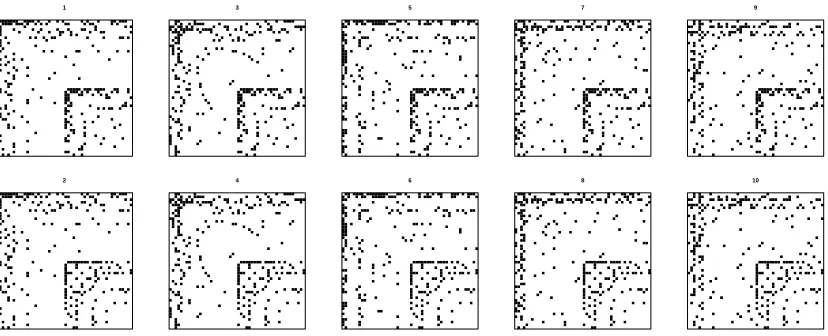
In our second study, we consider a more structured pattern withK = 10graphs. Each graphical model consists ofp= 50variables. Figure 3 shows the heat maps of the 10 adjacency matrices. This structured pattern is constructed as follows: we first generate the adjacency matrices corresponding to five distinctp-dimensional scale-free networks, so that the adjacency matrices in each column of the plot are the same. Next, we replace the connectivity structure of the bottom right diagonal block of sizep/2byp/2in each adjacency matrix with that of another two distinctp/2-dimensional scale-free networks, so that graphical models in each column exhibit the same connectivity pattern except in the bottom right diagonal block of their adjacency matrices. Note that by replacing the connectivity structure among the second half of the nodes, the relationships between the first half and the second half of the nodes are also altered. In summary, this structured pattern illustrates how different subsets of the edge sets across multiple graphical models can be similar, as well as exhibit differences in their topologies. To the best of our knowledge, such complex relationships have not been studied in the literature. In this setting, the proportion of shared non-edges (common zeros in the precision matrices) among all graphical models is about 60%.
Given the adjacency matrix or equivalently the edge set Ek, we generate the covariance and inverse covariance matrices in the same way as in the first simulation study. The input sparsity pattern G supplied for JSEM and the graph U required in MGGM are defined according to the pattern in Figure 3. We also study the effect of misspecification inG by varyingρ= 0,0.2,0.4,0.6, each corresponding to having only(1−ρ)∗100%of the information inG being correct for JSEM. At each level of pattern misspecification, we generatednk = 100independent samples for each
1 3 5 7 9
2 4 6 8 10
Figure 3: Simulation study 2: image plots of the adjacency matrices from all graphical models. Graphs in the same row share the same connectivity pattern at the bottom right block, whereas graphs in the same column share the same pattern at remaining locations.
graphical models to group. Asρincreases (0< ρ≤0.4), JSEM still performs the best despite the incorrectly specifiedG, while other methods perform not much better than the separate estimation method Glasso. Whenρ= 0.6, JSEM starts suffering from the large amount of pattern misspecifi-cation as well and performing not much better than separate estimation. Note at such highρvalues, the assumption of the presence of any related structures across graphical models becomes tenuous and therefore one is better off employing a separate estimation method for each graph.
Next, we examined the finite sample performance of different methods in identifying the true graphs and estimating the precision matrices at the optimal choice of tuning parameters. Table 2 shows the deviance measures between the estimated and the true precision matrices based on 50 replications for varying levels of pattern misspecification. Forρ ≤ 0.4, JSEM achieves a good balance between FP and FN, and yields the highestF1score and lowest Frobenius norm loss.
JEM-G is also very competitive in controlling false positive edges and comes next in overall performance. MGGM benefits from knowing the grouping structures and has comparable performance to JEM-G. In all cases, GGL achieves low FN, but very high FP, thus resulting in lowF1scores. Whenρ= 0.6,
the advantage of using a joint estimation method begins to diminish due to the high heterogeneity and separate estimation is recommended.
4.3 Simulation Study 3
Finally, we illustrate how direction consistency helps improve the estimation of graphical models using the previous two experimental settings. Table 3 presents the performance of thresholded JSEM whenG is moderately misspecified with individual to common ratioρ = 0.3, based on 50 replications. Note that we used a larger sample sizenk = 200in both settings to ensure that the
0.0 0.2 0.4 0.6 0.8 1.0
0.0
0.2
0.4
0.6
0.8
1.0
False positive rate
T
rue positiv
e r
ate
0.0 0.2 0.4 0.6 0.8 1.0
0.0
0.2
0.4
0.6
0.8
1.0
False positive rate
T
rue positiv
e r
ate
0.0 0.2 0.4 0.6 0.8 1.0
0.0
0.2
0.4
0.6
0.8
1.0
False positive rate
T
rue positiv
e r
ate
0.0 0.2 0.4 0.6 0.8 1.0
0.0
0.2
0.4
0.6
0.8
1.0
False positive rate
T
rue positiv
e r
ate
Figure 4: Simulation study 2: ROC curves for sample size nk = 100: Glasso (dotted in black),
JEM-G (dotdash in blue), GGL (solid in red), MGGM (dashed in purple), JSEM (long-dash in green). The misspecification ratioρ varies from (left to right): 0,0.2(top row) and0.4,0.6(bottom row).
positive edges with only a small loss in the presence of false negative edges. One may notice the slight increase in Frobenius norm loss for thresholded JSEM, which is likely due to the increased presence of false negative edges. Nevertheless, the thresholded version of JSEM obtains higherF1
scores, indicating an overall improvement in the structural estimation of all graphs.
ρ Method FP FN SHD F1 FL
0
Glasso 154(4) 38(1) 192(4) 0.51(0.01) 0.60(0.005) JEM-G 86(3) 36(2) 122(3) 0.62(0.01) 0.31(0.01) GGL 144(3) 39(1) 184(4) 0.52(0.01) 0.37(0.01) MGGM 30(2) 67(1) 97(2) 0.59(0.01) 0.36(0.01) JSEM 21(2) 42(2) 63(3) 0.75(0.01) 0.28(0.01)
0.2
Glasso 164(3) 47(1) 211(4) 0.53(0.01) 0.59(0.005) JEM-G 92(3) 57(2) 149(3) 0.59(0.01) 0.35(0.01) GGL 155(3) 48(1) 203(3) 0.53(0.01) 0.37(0.01) MGGM 94(3) 64(1) 158(4) 0.56(0.01) 0.37(0.01) JSEM 32(3) 64(2) 96(3) 0.67(0.01) 0.32(0.01)
0.4
Glasso 159(3) 59(1) 218(4) 0.55(0.01) 0.57(0.005) JEM-G 100(3) 77(2) 177(3) 0.56(0.01) 0.37(0.01) GGL 149(3) 61(2) 210(4) 0.55(0.01) 0.37(0.01) MGGM 119(3) 65(1) 184(3) 0.58(0.01) 0.37(0.01) JSEM 49(3) 84(2) 132(3) 0.62(0.01) 0.36(0.01)
0.6
Glasso 176(4) 73(2) 249(4) 0.54(0.01) 0.55(0.01) JEM-G 94(3) 109(2) 203(3) 0.52(0.01) 0.39(0.01) GGL 165(4) 76(2) 241(4) 0.54(0.01) 0.39(0.01) MGGM 109(3) 95(2) 204(4) 0.55(0.01) 0.39(0.01) JSEM 50(3) 123(2) 173(4) 0.52(0.01) 0.38(0.01)
Table 2: Performance of different regularization methods for estimating graphical models in Simu-lation Study 2: average FP, FN, SHD, F1 and FL (SE) for sample sizenk= 100. The best
cases are highlighted in bold.
Design Method FP FN SHD F1 FL
K = 5, p= 100,
G ={1,2,3,4,5}
JSEM 84(6) 12(1) 96(6) 0.71(0.01) 0.16(0.01) ThJSEM 29(4) 17(1) 46(4) 0.83(0.01) 0.16(0.01) K = 10, p= 40,
G as in Figure 3
JSEM 32(2) 5(0.7) 37(2) 0.78(0.01) 0.17(0.01) ThJSEM 20(2) 8(0.7) 28(2) 0.82(0.01) 0.19(0.01)
Table 3: Performance of JSEM and thresholded JSEM with misspecified groups (ρ = 0.3): av-erage FP, FN, SHD, F1 and FL (SE) for sample size nk = 200. The better cases are
highlighted in bold.
5. Applications
To illustrate the proposed joint estimation method in inferring real-world networks, we applied JSEM to a climate data set to study relationships between climate defining variables at multiple locations in North America, as well as a breast cancer gene expression data extracted from The Cancer Genome Atlas project (TCGA, 2012).
5.1 Application to Climate Modeling
Recent assessments from the Intergovernmental Panel on Climate Change (IPCC, Stocker et al., 2013) indicate multiple lines of evidence for climate change in the past century and these changes have caused significant impacts on natural and human systems. One common approach towards understanding the climate system has been attribution studies of detected changes to internal and external forcing mechanisms (such as solar radiation, greenhouse gases, etc.) using simulated cli-mate models. Lozano et al. (2009) used spatial-temporal modeling to study the attribution of clicli-mate defining mechanisms from observed data. In this work, we provide an alternative to learning the complex interactions among climate defining factors exhibited across different climate zones based on observed data.
The data used in this study are monthly measurements from January 2001 to June 2005 on 16 variables including mean temperature (TMP), diurnal temperature range (DTR), maximum and min-imum temperature (TMX, TMN), precipitation (PRE), vapor pressure (VAP), cloud cover (CLD), rain days (WET), potential evapotranspiration (PET), frost days (FRS), greenhouse gases (carbon dioxide (CO2), carbon monoxide (CO), methane (CH4), hydrogen (H2)), aerosols (AER) and solar radiation (SOL) from CRU (http://www.cru.uea.ac.uk/cru/data), NOAA (http://
www.esrl.noaa.gov/gmd/dv/ftpdata.html), NASA (http://disc.sci.gsfc.nasa.
gov/aerosols) and NCDC (ftp://ftp.ncdc.noaa.gov/pub/data/nsrdb-solar/).
The data are organized as a 2.5 degree latitude by 2.5 degree longitude grid across North Amer-ica. To avoid complications from any seasonality or autocorrelation of the data, we aggregated the monthly time series into bins of 3-month intervals and took first differences of the quarterly data. The data after differencing were further normalized. Details on the pre-processing steps are in-cluded in Appendix D. Next, we randomly selectedK = 27locations spanning all types of climate from the 2.5 by 2.5 degree grid of North America (see Figure 5). This gives us ann×pmatrix at each of the 27 locations, corresponding ton= 17observations for thep = 16climate defining variables. At each location, the conditional dependency network is of dimensionp×p, which has
16×15/2 = 120edges to be inferred.
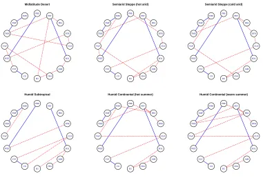
Our goal is to infer the conditional dependency networks forall locations simultaneouslybased on available spatial information, obtained from the classification of climate zones in Peel et al. (2007). Specifically, we assume that AER and SOL have one common connectivity pattern with other variables in the geographical south of North America and another common pattern in the north. The definition of the south and north is given in Figure 5. Variables on greenhouse gases (CO2, CO, CH4 and H2) are assumed to interact with other variables (except AER and SOL) in the same fashion within each of the four climate groups, that is Mid-latitude Desert, Semiarid Steppe, Humid Subtropical and Humid Continental. The connectivity patterns among all remaining variables are assumed to be the same within each of the six distinct climate zones in Figure 5.
● ●
● ● ●
● ●
●
●
Midlatitude Desert Semiarid Steppe (hot arid) Semiarid Steppe (cold arid) Humid Subtropical
Humid Continental (hot summer) Humid Continental (warm summer)
Figure 5: The selected 27 locations based on climate classification. The solid line separates the south and north of North America and corresponds to latitude 39 N.
and Samworth, 2013) to identify the interaction networks at the 27 locations. To perform stability selection, we ran our method 50 times on two randomly drawn complementary pairs of sizes 8 and 9, and kept only edges that are selected over 70% of the time.
Midlatitude Desert
CLD DTR FRS PET PRE TMN TMP
TMX
VAP
WET
CO2 CO
H2 CH4
AER SOL
Semiarid Steppe (hot arid)
CLD DTR FRS PET PRE TMN TMP
TMX
VAP
WET
CO2 CO
H2 CH4
AER SOL
Semiarid Steppe (cold arid)
CLD DTR FRS PET PRE TMN TMP
TMX
VAP
WET
CO2 CO
H2 CH4
AER SOL
Humid Subtropical
CLD DTR FRS PET PRE TMN TMP
TMX
VAP
WET
CO2 CO
H2 CH4
AER SOL
Humid Continental (hot summer)
CLD DTR FRS PET PRE TMN TMP
TMX
VAP
WET
CO2 CO
H2 CH4
AER SOL
Humid Continental (warm summer)
CLD DTR FRS PET PRE TMN TMP
TMX
VAP
WET
CO2 CO
H2 CH4
AER SOL
Figure 6: Estimated climate networks at the six distinct climate zones using JSEM, with edges shared across all locations blue solid and differential edges red dashed.
warm summer), whereas those with dramatically different climate show significantly different con-nectivity patterns. These common and individual interactions can prove critical in understanding the mechanisms of climate defining, and facilitate decision making in maintaining the best environ-mental results.
5.2 Application to Breast Cancer
Breast cancer is the most common cancer in women worldwide, with nearly 1.7 million new cases diagnosed in 2012 (second most common cancer overall). This represents about 12% of all new can-cer cases and 25% of all cancan-cers in women (Ferlay et al., 2013). Breast cancan-cer is hormone related and this leads to a basic classification of cancer cells. Specifically, a cancer is called estrogen-receptor-positive (or ER+) if it has receptors for estrogen, and hence the cells receive signals from estrogen that could promote their growth. It is estimated that about 80% of all breast cancer cases are ER+ and they are more likely to respond to hormone therapy. Further, ER+ status is associated with better survival rates, especially if the cancer is diagnosed early. On the other hand, the ER-status lacks the estrogen receptor and in general exhibits poorer survival rates. Note that the pres-ence/absence of other hormone receptors (progesterone and HER2) also play an important role in breast cancer tumor classification, therapeutic strategies and survival rates.
overall small sample size, we first reduced the number of variables by focusing on a subset of the genes that are present in the 44 KEGG pathways in Table 4. These pathways correspond to the major signaling and biochemical ones that have been reported in the literature of playing a significant role in all cancer types. This leaves for further consideration 800 genes with 403 samples from the ER+ and 117 from the ER- classes.
The structural similarity between the networks for ER+ and ER- status was defined based on the third column in Table 4, which indicates whether the pathway is significantly enriched when testing ER+ vs ER- status via NetGSA (Ma et al., 2016), and complemented through literature searches. If one pathway is not significantly enriched, then the genes belonging to the pathway are considered to share a common structure under both ER+ and ER- status. However, due to overlaps amongst pathways (since some of their members are assigned to multiple ones in the KEGG database), only genes that did not belong to any of the differential pathways were used to define the common structure. The remaining genes are assumed to have distinct structures under the two conditions.
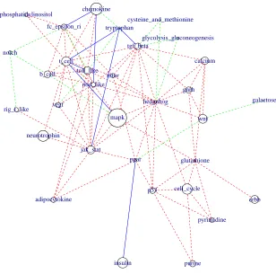
We then used BIC on the normalized data to select the tuning parameter λ for the proposed JSEM. At the optimalλ, we applied our method coupled with complementary pairs stability selec-tion (Shah and Samworth, 2013) to identify the interacselec-tion networks for the ER+ and ER- classes, respectively. Due to the large number of variables, visualization of the estimated networks at the in-dividual gene level is challenging. Instead, we examine the interactions among pathways in Figure 7 to gain insight into their co-regulation behavior. The weighted pathway level network is defined as follows. Let each node in the network represent one pathway, with size proportional to the size of the corresponding pathway. A weighted edge between two pathwaysP1 andP2 is defined as the
number of nonzero partial correlations between genes inP1and those inP2(normalized by the sizes
of the two pathways). Links visualized in Figure 7 are the top 5% of the weighted edges, where ranking is based on edge weights. Note pathways that are isolated from all others were removed.
The first thing to note is that structural information provided enables us to estimate a much more dense graph than either separate estimation or an agnostic method like JEM-G (see Figure 12 in Ap-pendix D), which in turn aids biological interpretation. We focus next on the interactions between pathways, as shown in Figure 7. The central role of known cancer related pathways—TGF-β, p53, MAPK and hedgehog—is apparent. Further, we see high degree of interconnections between sig-naling and biochemical pathways including glycolysis gluconeogenesis, pyrimidine, cysteine and methionine, and tryptophan, which is expected due to the impact of energy metabolism in tumor growth and progression. One surprising finding is that the p53 pathway is connected only in the ER+ class, but we suspect that this may be the case due to the big discrepancy in terms of available samples for the ER+ and ER- classes and the large number of genes present. In summary, the pro-posed method captures established cross-talk patterns between various signaling and biochemical pathways, which is not the case with competing methods or with separate estimation.
6. Discussion
mis-Vertex id Vertex names KEGG names Status 1 glycolysis gluconeogenesis glycolysis gluconeogenesis TRUE 2 citrate cycle tca cycle citrate cycle tca cycle FALSE 3 pentose phosphate pentose phosphate pathway TRUE 4 fructose and mannose fructose and mannose metabolism TRUE
5 galactose galactose metabolism TRUE
6 fatty acid fatty acid metabolism FALSE
7 oxidative phosphorylation oxidative phosphorylation FALSE
8 purine purine metabolism TRUE
9 pyrimidine pyrimidine metabolism TRUE
10 glycine serine and threonine glycine serine and threonine metabolism FALSE 11 cysteine and methionine cysteine and methionine metabolism TRUE 12 valine leucine and isoleucine valine leucine and isoleucine degradation TRUE
13 lysine lysine degradation FALSE
14 arginine and proline arginine and proline metabolism FALSE
15 tryptophan tryptophan metabolism FALSE
16 beta alanine beta alanine metabolism TRUE
17 glutathione glutathione metabolism TRUE
18 starch and sucrose starch and sucrose metabolism TRUE 19 amino sugar and nucleotide sugar amino sugar and nucleotide sugar metabolism FALSE
20 ppar ppar signaling pathway TRUE
21 mapk mapk signaling pathway FALSE
22 erbb erbb signaling pathway TRUE
23 calcium calcium signaling pathway FALSE
24 chemokine chemokine signaling pathway TRUE 25 phosphatidylinositol phosphatidylinositol signaling system FALSE
26 cell cycle cell cycle TRUE
27 p53 p53 signaling pathway TRUE
28 mtor mtor signaling pathway FALSE
29 wnt wnt signaling pathway FALSE
30 notch notch signaling pathway FALSE
31 hedgehog hedgehog signaling pathway TRUE
32 tgf beta tgf beta signaling pathway TRUE
33 vegf vegf signaling pathway FALSE
34 toll like toll like receptor signaling pathway TRUE 35 nod like nod like receptor signaling pathway TRUE 36 rig i like rig i like receptor signaling pathway FALSE
37 jak stat jak stat signaling pathway TRUE
38 t cell t cell receptor signaling pathway FALSE 39 b cell b cell receptor signaling pathway FALSE 40 fc epsilon ri fc epsilon ri signaling pathway TRUE 41 neurotrophin neurotrophin signaling pathway FALSE
42 insulin insulin signaling pathway FALSE
43 gnrh gnrh signaling pathway TRUE
44 adipocytokine adipocytokine signaling pathway TRUE
●
●
●
●
● ●
●
●
●
● ●
●
● ●
●
●
●
●
●
●
●
●
●
●
●
●
●
●
●
glycolysis_gluconeogenesis
galactose
purine pyrimidine cysteine_and_methionine
tryptophan
glutathione ppar
mapk
erbb calcium
chemokine phosphatidylinositol
cell_cycle p53
mtor
wnt notch
hedgehog tgf_beta
vegf
toll_like
nod_like
rig_i_like
jak_stat t_cell
b_cell fc_epsilon_ri
neurotrophin
insulin
gnrh
adipocytokine
Figure 7: Estimated pathway networks for the ER+ and ER- classes using JSEM, with edges shared across all locations blue solid and differential edges red dashed (ER+) / green dashed (ER-).
specified structured sparsity pattern. On the other hand, if more structural information is available, one may generalize the group lasso penalty to incorporate additional structural constraints.
The theoretical guarantees of JSEM rely on two important, but standard in the literature, as-sumptions: the restricted eigenvalue assumption (A1) and the uniform IC assumption in (A3). In practice, it might be difficult to verify whether these assumptions are fulfilled, especially the more stringent assumption (A3). For the latter condition, Meinshausen and Yu (2009) observe that the irrepresentability condition (a variant of A3) may be violated in practical settings in the presence of highly correlated variables; nevertheless, the lasso estimates are still`2consistent, under (A1).
The authors would like to thank two anonymous reviewers for helpful comments and suggestions. The work of GM was supported in part by NSF awards DMS-1228164 and DMS-1545277 and NIH award 7R21GM10171903.
Appendix A. Proof of Theorem 1
To prove the rate of convergence in Theorem 1, we look at three key steps: nodewise regression in subsection A.1, selecting the edge set in A.2 and maximum likelihood refitting in A.3. More information can be found in Appendix E. When it is clear, we shall useP
k as a short notation for
PK
k=1.
A.1 Regression
For j 6= i, g ∈ Gij, k ∈ g, letεk
i = Xki −
P
j6=iθ0k,ijXkj. Let ha, bi represent the inner product
between two vectorsaandb. Denoteζijk =hεki,Xkji/nandζ[ijg] = (ζijk)k∈g ∈ R|g|. Consider the
random eventA= T
i,j6=i,g
Aijg, whereAgij ={2kζij[g]k ≤λgij}. By Lemma E.2, if we chooseλgij as
λgij ≥max k∈g
2
q nωk
0,ii
p
|g|+√π
2
p
qlogG0
(10)
withq > 1, thenP(A) ≥1−2pG1−0 q. We first present the following proposition that establishes
oracle bounds forΘˆi−Θ0,iunder the chosenλgij.
Proposition A.1 Fori= 1, . . . , p, consider the problem(2)and chooseλgij as in(10). LetΘˆi be the solution to problem(2). If Assumption (A1) holds withκ2 =κ2(s0), then for any solutionΘˆiof problem(2), we have on the eventA
X
j6=i,g∈Gij
kθˆ[ijg]−θ[0g,ij] k ≤ 16 κ2λ
min
X
(j,g)∈J(Θ0,i)
(λgij)2, (11)
M( ˆΘi)≤
64φmax
κ2λ2 min
X
(j,g)∈J(Θ0,i)
(λgij)2, (12)
whereλmin = min
i,j6=i,g∈Gijλ
g
ij,M( ˆΘi) =|J( ˆΘi)|andφmaxis the maximal eigenvalue of(Xk)TXk/n
for allk= 1,· · ·, K. If, in addition, Assumption (A1) holds withκ2(2s0), then for any solutionΘˆi of problem(2)we have that
kΘiˆ −Θ0,ikF ≤
4√10
κ2(2s 0)
P
(j,g)∈J(Θ0,i)(λ
g ij)2
λmin
√ si
. (13)
By Assumption (A2),ω0k,ii ≥φmin(Ωk0) = φ−1max(Σk0)≥d0for alli, k. Thus, (10) implies that
we can chooseλgij =λmaxas
λmax=
2
√ nd0
p
|gmax|+
π √
2
p
qlogG0
withq >1for all 3-tuples(i, j, g). Then we can rewrite the oracle inequalities in (12) and (13) as M( ˆΘi)≤ 64φmax
κ2 si, (15)
kΘiˆ −Θ0,ikF ≤
8√10
κ2(2s 0)
√ d0
p
|gmax|+
π √
2
p
qlogG0
r si
n. (16)
Detailed proof of Proposition A.1 follows similarly to that of Theorem 3.1 in Lounici et al. (2011) and can be found in Appendix E.
A.2 Selecting Edge Set
Given the estimates Θˆi (i = 1, . . . , p), defineEˆk as in (3) the estimated set of edges in graph
k= 1, . . . , K. For everyk, letΩek = diag(Ωk0) + Ωk
0,Ek
0∩Eˆk
andΣek= (Ωek)−1. Let
Cbias=
8√10c0
κ2(2s 0)
√ d0
.
The following corollary is an immediate result of (15) and (16).
Corollary A.1 ConsiderEˆk(k = 1, . . . , K)selected in(3). Suppose all conditions in Theorem 1 are satisfied. Chooseλgij =λmaxas defined in(14)withq >1. Then we have on the eventA
|Eˆk| ≤ 64φmax κ2(s
0)
S0, k= 1, . . . , K, (17)
and 1
K X
k
kΩek−Ωk0kF ≤
1
√ K
nX
k
kΩek−Ωk0k2F o1/2
≤Cbias
r S0
nK
p
|gmax|+
π √
2
p
qlogG0
,
(18)
whereG0is the maximum number of groups in allpregressions,S0is the total number of relevant
groups, and|gmax|is the maximum group size.
The bound in (17) says that the cardinality of the estimated set of edges is at most of the order ofS0 and proves essential in controlling the error rate of the maximum likelihood estimateΩˆkin
the refitting step. Further, the second inequality in (18) implies nX
k
kΩek−Ωk0k2F o1/2
≤τ1d0,
provided the sample sizensatisfies for0< τ1 <1,
n≥S0
p
|gmax|+
π √
2
p
qlogG0
2 Cbias
τ1d0
2 .
It follows immediately that on the eventA, we can bound the spectrum ofΩek(k = 1, . . . , K)as follows. For a symmetric matrix A, let kAk represent the spectral norm ofA, which is equal to φmax(A). By definition,
φmin(Ωek) = min
v:vTv=1v
T
e
Ωkv = min v:vTv=1{v
TΩk
Sinceφmin(Ωk0)≥d0by Assumption (A2), we have
φmin(Ωek)≥φmin(Ωk0)− kΩek−Ωk0k ≥φmin(Ωk0)− kΩek−Ωk0kF ≥φmin(Ωk0)−
n X
k
kΩek−Ωk0k2F o1/2
≥(1−τ1)d0 >0, (19)
In addition, we have an upper bound for the maximum eigenvalue ofΩek,
φmax(Ωek)≤φmax(Ωk0) +kΩek−Ωk0k ≤φmax(Ωk0) +kΩek−Ωk0kF ≤φmax(Ωk0) +
n X
k
kΩek−Ωk0k2F o1/2
≤c0+τ1d0 <∞. (20)
A.3 Refitting
LetΩˆk(k= 1, . . . , K)be defined in (4) and
rn=Cbias
r S0
n
p
|gmax|+
π √
2
p
qlogG0
. (21)
Proof[of Theorem 1.] In view of Corollary A.1, it suffices to show that X
k
kΩˆk−Ωekk2F ≤O rn2
,
since by Cauchy-Schwarz inequality,
1
K X
k
kΩˆk−ΩekkF ≤
1
√ K
nX
k
kΩˆk−Ωekk2F o1/2
,
and by triangle inequality,
1
K X
k
kΩˆk−Ωk0kF ≤ 1 K
X
k
kΩˆk−ΩekkF +
1
K X
k
kΩek−Ωk0kF.
Fork= 1, . . . , K, let∆k= Ωk−Ωek∈M(p, p)and∆ˆk= ˆΩk−Ωek. Let Q(Ω) =X
k
n
tr( ˆΣkΩk)−log det(Ωk)−tr( ˆΣkΩek) + log det(Ωek) o
.
Since ( ˆΩk)Kk=1 minimizes Q(Ω), ( ˆ∆k)Kk=1 minimizes G(∆) = Q(Ω + ∆)e . Recall the definition SE+ ={Γ ∈Rp×p : Γ0andΓ
ij = 0, for all(i, j)∈/ Ewherei6=j}. Fork= 1, . . . , K, define
a sequence of convex sets
Un(Ωek) ={Γ−Ωek|Γ∈ S+ˆ
Ek}.
The main idea of the proof is as follows. For a sufficiently largeM >0, consider the set Tn={(∆1, . . . ,∆K) : ∆k ∈ Un(Ωek),
X
k
Write 0p×p the zero matrix in M(p, p). It is clear that G(∆) is a convex function and G( ˆ∆) ≤
G(0p×p) = 0.Thus if we can show inf∆∈TnG(∆) > 0, the minimizer ∆ˆ must be inside the
ball defined by Tn. That is P
kk∆ˆkk2F ≤ M rn2.To see this, note that the convexity of Q(Ω)
implies thatinf∆∈TnQ(Ω + ∆)e > Q(Ω) = 0e .There exists therefore a local minimizer in the ball {Ωek+ ∆k :
P
kk∆kk2F ≤M r2n}, or equivalently,
P
kk∆ˆkk2F ≤M rn2.
In the remainder of the proof, we focus on
G(∆) =X k
n
tr( ˆΣk∆k)−log det(Ωek+ ∆k) + log det(Ωek) o
.
Applying Taylor expansion to the logarithm terms in the above equation, we have
log det(Ωek+ ∆k)−log det(Ωek)
=tr(Σek∆k)−vec(∆k)T Z 1
0
(1−t)(Ωek+t∆k)−1⊗(Ωek+t∆k)−1dt
vec(∆k),
where⊗is the Kronecker product, andvec(∆k)is∆kvectorized to match the dimensions of the Kronecker product. Therefore, we can rewriteG(∆) =L1−L2+L3, with
L1=
X
k tr
( ˆΣk−Σk0)∆k ,
L2=
X
k tr
(Σek−Σk0)∆k ,
L3=
X
k
vec(∆k)T
Z 1
0
(1−t)(Ωek+t∆k)−1⊗(Ωek+t∆k)−1dt
vec(∆k).
Next we bound each term separately.
Recall for every k, Σk0 and Σˆk represent the correlation and the sample correlation matrix, respectively. By Lemma 14 of Zhou et al. (2011) [see details on page 3003],
P
n
|σˆijk −σk0,ij| ≥t o
≤exp
− 3nt
2
10{1 + (σ0k,ij)2}
≤exp
−3nt
2
20
, (22)
for0≤t≤ {1 + (σk0,ij)2}/2. Then the union sum inequality and (22) imply that, with probability tending to 1,
max k,i6=j|σˆ
k
ij −σ0k,ij| ≤c1
r
1
nK
p
|gmax|+
π √
2
p
qlogG0
,
provided that the sample size satisfies
n≥ 4c
2 1
K
p
|gmax|+
π √
2
p
qlogG0
2 ,
where c1 > 0 is a constant. Write∆k = ∆k,++ ∆k,− such that∆k,+ = diag(∆k) and∆k,−
consists of the off-diagonal entries of∆k. Then
|L1| ≤
X
k
X
i6=j
|σˆijk −σ0k,ij||∆kij| ≤c1
r
1
nK
p
|gmax|+
π √
2
p
qlogG0
X
k
By Cauchy-Schwarz inequality and the definition of∆k ∈ Un(Ωek), X
k
k∆k,−k1 ≤X
k
(2|Eˆk|)1/2k∆k,−kF ≤max k (2|
ˆ
Ek|)1/2√KX
k
k∆kk2
F
1/2 .
Using the bound ofEˆkin (17) and the definition ofrn, we obtain
|L1| ≤c1
r
1
n
p
|gmax|+
π √
2
p
qlogG0
8√2φmaxS0
κ(s0)
X
k
k∆kk2F1/2
= 8
√
2c1
√ φmax
Cbiasκ(s0)
rn
M rn21/2 = 8
√
2c1
√ φmax
Cbiasκ(s0)
√
M rn2, (23)
where the first equality in (23) follows from the definition ofrnin (21).
Using results from (19) and (18) together with Cauchy-Schwarz inequality, the second termL2
can be bounded by
|L2| ≤
X
k
|hΣek−Σk0,∆ki| ≤ X
k
kΣek−Σk0kFk∆kkF ≤ X
k
k∆kkF
kΩek−Ωk0kF φmin(Ωek)φmin(Ωk0)
(24)
≤ 1
(1−τ1)d02
X
k
k∆kk2F1/2X
k
kΩek−Ωk0k2F 1/2
≤ √
M r2
n (1−τ1)d02
,
where the last inequality in (24) comes from the rotation invariant property of the Frobenius norm. Finally we bound L3. Suppose for a small constant0 < τ2 < 1 such thatτ1 +τ2 < 1, the
sample sizensatisfies
n≥M S0
p
|gmax|+
π √
2
p
qlogG0
2 Cbias
τ2d0
2 ,
then√M rn≤τ2d0. By (20),φmax(Ωek)is bounded above byc0+τ1d0. Therefore for∆∈ Tn, φmax(Ωek+ ∆k)≤c0+τ1d0+k∆kk ≤c0+τ1d0+k∆kkF
≤c0+τ1d0+
X
k
k∆kk2F1/2 ≤c0+ (τ1+τ2)d0,
φmin(Ωek+ ∆k)≥(1−τ1)d0− k∆kk ≥(1−τ1)d0− k∆kkF ≥(1−τ1)d0−
X
k
k∆kk2F1/2≥(1−τ1−τ2)d0>0.
For Ωek and∆k defined above, Zhou et al. (2011) showed thatΩek+t∆k 0, t ∈ [0,1], for all k= 1, . . . , K on the eventA. Thus, following similar arguments as in Rothman et al. (2008, page 502), we have
|L3| ≥
1 2
X
k
φ2min(Ωek+ ∆k)−1k∆kk2F =
1 2
X
k
φ−2max(Ωek+ ∆k)k∆kk2F
≥ M r
2
n
2(c0+τ1d0+τ2d0)2
Combining the above three bounds, we thus have
G(∆)≥ |L3| − |L1| − |L2|
≥ M r
2
n
2(c0+τ1d0+τ2d0)2
− 8
√
2c1
√ φmax
Cbiasκ(s0)
√ M rn2−
√ M rn2
(1−τ1)d02
≥M rn2
1
2(c0+τ1d0+τ2d0)2
−8c1 √
2φmax
Cbiasκ(s0)
1
√ M −
1 (1−τ1)d02
√ M
>0,
forM sufficiently large.
Appendix B. Proof of Theorem 2
Consider the group lasso estimatorΘiˆ defined in (2). Since the problem (2) is a special case of the generic group lasso in Basu et al. (2015), we adapt their results in Theorem 4.1 to our design.
Proof LetXi be the block diagonal matrix composed of all variables butXki (k= 1, . . . , K), that
is
Xi =
X1−i
. ..
XK−i
.
After rearranging the columns of Xi, we assume without loss of generality Xi = (Xi,(1),Xi,(2))
such that
Xi,(1)= diag(X1I1, . . . ,XKIK)
is the sub-matrix consisting of all relevant variables. Denote the Gram matrix
C= 1
nX
T i Xi=
C11 C12
C21 C22
withC11 = Xi,T(1)Xi,(1)/nandC22 = Xi,T(2)Xi,(2)/n. C12 andC21 are also defined accordingly.
Note due to the block diagonal structure ofXi,(1),C11is also block diagonal.
Now consider interchanging the columns ofXisuch that
˜
Xi=Xidiag(R1, R2) = (Xi,(1)R1,Xi,(2)R2) = ( ˜Xi,(1),X˜i,(2)),
where the columns ofX˜i,(1) andX˜i,(2) are ordered in groups of variables. Here Rl is the
prod-uct of elementary column switching matrices and satisfies R−1l = RT
l (l = 1,2). Note R1 ∈
M(Pk|Ik|,Pk|Ik|). Based onX˜i, we can defineC˜11,C˜21andC˜22similarly as above. The
advan-tage of usingX˜ias the design matrix is that it orders the variables based on the grouping structures,
and is in the form of the generic group lasso design in Basu et al. (2015). It is thus more straight-forward to adapt their results usingX˜i. Moreover, since each group of variables(j, g)corresponds to regression coefficients at the same (i, j) position across different models ing, the matrix C˜11