Robust Near-Separable Nonnegative Matrix Factorization
Using Linear Optimization
Nicolas Gillis∗ [email protected]
Department of Mathematics and Operational Research Facult´e Polytechnique, Universit´e de Mons
Rue de Houdain 9, 7000 Mons, Belgium
Robert Luce† [email protected]
Institut f¨ur Mathematik, MA 3-3 Technische Universit¨at Berlin
Straße des 17. Juni 136 - 10623 Berlin, Germany
Editor:Gert Lanckriet
Abstract
Nonnegative matrix factorization (NMF) has been shown recently to be tractable under the separability assumption, under which all the columns of the input data matrix be-long to the convex cone generated by only a few of these columns. Bittorf, Recht, R´e and Tropp (‘Factoring nonnegative matrices with linear programs’, NIPS 2012) proposed a linear programming (LP) model, referred to as Hottopixx, which is robust under any small perturbation of the input matrix. However, Hottopixx has two important drawbacks: (i) the input matrix has to be normalized, and (ii) the factorization rank has to be known in advance. In this paper, we generalize Hottopixx in order to resolve these two drawbacks, that is, we propose a new LP model which does not require normalization and detects the factorization rank automatically. Moreover, the new LP model is more flexible, sig-nificantly more tolerant to noise, and can easily be adapted to handle outliers and other noise models. Finally, we show on several synthetic data sets that it outperforms Hottopixx while competing favorably with two state-of-the-art methods.
Keywords: nonnegative matrix factorization, separability, linear programming, convex optimization, robustness to noise, pure-pixel assumption, hyperspectral unmixing
1. Introduction
Nonnegative matrix factorization (NMF) is a powerful dimensionality reduction technique as it automatically extracts sparse and meaningful features from a set of nonnegative data vectors: Given n nonnegative m-dimensional vectors gathered in a nonnegative matrix
M ∈Rm+×nand a factorization rankr, NMF computes two nonnegative matricesW ∈Rm ×r
+
and H ∈ Rr+×n such that M ≈ W H. In this way, the columns of the matrix W form a basis for the columns of M since M(:, j) ≈ Prk=1W(:, k)H(k, j) for all j. Moreover, the nonnegativity constraint on the matrices W and H leads these basis elements to represent
∗. This work was carried out when NG was a postdoctoral researcher of the fonds de la recherche scientifique (F.R.S.-FNRS).
common localized features appearing in the data set as no cancellation can happen in the reconstruction of the original data. Unfortunately, NMF is NP-hard in general (Vavasis, 2009), and highly ill-posed; see Gillis (2012) and the references therein. However, if the input data matrixM is r-separable, that is, if it can be written as
M =W[Ir, H0]Π,
where Ir is the r-by-r identity matrix, H0 ≥ 0 and Π is a permutation matrix, then the problem can be solved in polynomial time, even if some noise is added to the separable matrixM (Arora et al., 2012a). Algebraically, separability means that there exists a rank-r
NMF (W, H)≥0 ofM where each column ofW is equal to some column ofM. Geometri-cally,r-separability means that the cone generated by the columns ofM hasrextreme rays given by the columns of W. Equivalently, if the columns ofM are normalized so that their entries sum to one,r-separability means that the convex hull generated by the columns of
M hasrvertices given by the columns ofW; see, e.g., Kumar et al. (2013). The separability assumption is far from being artificial in several applications:
• In text mining, where each column of M corresponds to a word, separability means that, for each topic, there exists a word associated only with that topic; see Arora et al. (2012a,b).
• In hyperspectral imaging, where each column of M equals the spectral signature of a pixel, separability means that, for each constitutive material (“endmember”) present in the image, there exists a pixel containing only that material. This assumption is referred to as thepure-pixel assumption, and is in general satisfied for high-resolution hyperspectral images; see Bioucas-Dias et al. (2012) and the references therein.
• In blind source separation, where each column of M is a signal measure at a given point in time, separability means that, for each source, there exists a point in time where only that source is active; see Chan et al. (2008); Chen et al. (2011) and the references therein.
Under the separability assumption, NMF reduces to identifying, among the columns of
M, the columns of W allowing to reconstruct all columns of M. In fact, given W, the matrixH can be obtained by solving a convex optimization problem minH≥0kM−W Hk.
In this paper, we consider the noisy variant of this problem, referred to asnear-separable
NMF:
(Near-Separable NMF) Given a noisy r-separable matrix M˜ = M +N with
M = W H = W[Ir, H0]Π where W and H0 are nonnegative matrices, Π is a permutation matrix and N is the noise, find a set K of r indices such that
˜
M(:,K)≈W.
Remark 1 (Nonnegativity of M˜) In the formulation of near-separable NMF, the input data matrix M˜ is not necessarily nonnegative since there is no restriction on the noise N. In fact, we will only need to assume that the noise is bounded, but otherwise it is arbitrary; see Section 2.
1.1 Notation
Let A ∈ Rm×n be a matrix and x ∈
Rm a vector. We use Matlab-style notation for indexing, for example,A(i, j) denotes the entry ofAin the i-th row andj-th column, while
A(:, j)∈Rm denotes thej-th column ofA. We use the following notation for various norms:
kxk1= m X
i=1
|x(i)|, kAk1 = max
kxk1≤1
kAxk1= max
j kA(:, j)k1,
kAks= m X
i=1
n X
j=1
|A(i, j)|, kAkF = v u u t
m X
i=1
n X
j=1
A(i, j)2.
1.2 Hottopixx, a Linear Programming Model for Near-Separable NMF
A matrix M is r-separable if and only if
M =W H =W[Ir, H0]Π = [W, W H0]Π
= [W, W H0]Π Π−1
Ir H0 0(n−r)×r 0(n−r)×(n−r)
Π
| {z }
X0∈ Rn+×n
=M X0, (1)
for some permutation Π and some matrices W, H0 ≥0. The matrix X0 is a n-by-n non-negative matrix with (n−r) zero rows such thatM =M X0. Assuming the entries of each column ofM sum to one, the entries of each column ofW and H0 have sum to one as well. Based on these observations, Bittorf et al. (2012) proposed to solve the following optimiza-tion problem in order to approximately identify the columns of the matrix W among the columns of the matrix ˜M =M +N where N is the noise with kNk1 ≤:
min X∈Rn+×n
pTdiag(X)
such that kM˜ −M X˜ k1≤2,
tr(X) =r, (2)
X(i, i)≤1 for all i,
X(i, j)≤X(i, i) for all i, j,
wherepis anyn-dimensional vector with distinct entries; see Algorithm 1 (in Bittorf et al., 2012, the authors use the notationk·k∞,1 for what we denote byk·k1).
Intuitively, the LP model1 (2) assigns a total weight r to the n diagonal entries of the variable X in such a way that ˜M can be well approximated using nonnegative linear
Algorithm 1 Hottopixx - Extracting Columns of a Noisy Separable Matrix using Linear Optimization (Bittorf et al., 2012)
Input: A normalized noisy r-separable matrix ˜M = W H+N ∈Rm+×n, the factorization
rank r, the noise level kNk1 ≤and a vector p∈Rn with distinct entries.
Output: A matrix ˜W such that ˜W ≈W (up to permutation). 1: Find the optimal solutionX∗ of (2).
2: LetK be the index set corresponding to the r largest diagonal entries ofX∗. 3: Set ˜W = ˜M(:,K).
combinations of columns of ˜M corresponding to positive diagonal entries of X. Moreover, the weights used in the linear combinations cannot exceed the diagonal entries of X since
X(:, j) ≤ diag(X) for all j. There are several drawbacks in using the LP model (2) in practice:
1. The factorization rankrhas to be chosen in advance. In practice the true factorization rank is often unknown, and a “good” factorization rank for the application at hand is typically found by trial and error. Therefore the LP above may have to be resolved many times.
2. The columns of the input data matrix have to be normalized in order for their entries to sum to one. This may introduce significant distortions in the data set and lead to poor performance; see Kumar et al. (2013) where some numerical experiments are presented.
3. The noise level kNk1 ≤has to be estimated.
4. One has to solve a rather large optimization problem with n2 variables, so that the
model cannot be used directly for huge-scale problems.
It is important to notice that there is no way to getting rid of both drawbacks 2. and 3. In fact, in the noisy case, the user has to indicate either
• The factorization rank r, and the algorithm should find a subset of r columns of ˜M
as close as possible to the columns ofW, or
• The noise level, and the algorithm should try to find the smallest possible subset of columns of ˜M allowing to approximate ˜M up to the required accuracy.
1.3 Contribution and Outline of the Paper
In this paper, we generalize Hottopixx in order to resolve drawbacks 1. and 2. above. More precisely, we propose a new LP model which has the following properties:
• Given the noise level , it detects the number r of columns of W automatically; see Section 2.
• It does not require column normalization; see Section 4.
• It is significantly more tolerant to noise than Hottopixx. In fact, we propose a tight ro-bustness analysis of the new LP model proving its superiority (see Theorems 2 and 6). This is illustrated in Section 5 on several synthetic data sets, where the new LP model is shown to outperform Hottopixx while competing favorably with two state-of-the-art methods, namely the successive projection algorithm (SPA) (Ara´ujo et al., 2001; Gillis and Vavasis, 2014) and the fast conical hull algorithm (XRAY) (Kumar et al., 2013).
The emphasis of our work lies in a thorough theoretical understanding of such LP based approaches, and the numerical experiments in Section 5 illustrate the proven robustness properties. An implementation for real-word, large-scale problems is, however, a topic outside the scope of this work (see Section 6).
2. Detecting the Factorization Rank Automatically
In this section, we analyze the following LP model:
min X∈Rn×n
+
pTdiag(X)
such that kM˜ −M X˜ k1≤ρ, (3)
X(i, i)≤1 for all i,
X(i, j)≤X(i, i) for all i, j,
where p haspositive entries and ρ >0 is a parameter. We also analyze the corresponding near-separable NMF algorithm (Algorithm 2) with an emphasis on robustness. The LP
Algorithm 2Extracting Columns of a Noisy Separable Matrix using Linear Optimization
Input: A normalized noisy r-separable matrix ˜M = W H +N ∈ Rm+×n, the noise level
kNk1 ≤, a parameter ρ >0 and a vectorp∈Rn with positive distinct entries.
Output: Anm-by-r matrix ˜W such that ˜W ≈W (up to permutation). 1: Compute an optimal solutionX∗ of (3).
2: LetKbe the index set corresponding to the diagonal entries ofX∗larger than 1−min(12 ,ρ). 3: W˜ = ˜M(:,K).
model (3) is exactly the same as (2) except that the constraint tr(X) =rhas been removed, and that there is an additional parameter ρ. Moreover, the vector p∈Rn in the objective function has to be positive, or otherwise any diagonal entry of an optimal solution of (3) corresponding to a negative entry ofpwill be equal to one (in fact, this reduces the objective function the most while minimizing kM−M Xk1). A natural value for the parameter ρ is
feasible. Hence, it is not clear a priori which value of ρ should be chosen. The reason we analyze the LP model (3) for different values of ρ is two-fold:
• First, it shows that the LP model (3) is rather flexible as it is not too sensitive to the right-hand side of the constraint kM −M Xk1 ≤ ρ. In other terms, the noise level does not need to be known precisely for the model to make sense. This is a rather desirable property as, in practice, the value of is typically only known/evaluated approximately.
• Second, we observed that taking ρ smaller than two gives in average significantly better results (see Section 5 for the numerical experiments). Our robustness analysis of Algorithm 2 will suggest that the best choice is to take ρ= 1 (see Remark 5).
In this section, we prove that the LP model (3) allows to identifying approximately the columns of the matrix W among the columns of the matrix ˜M for any ρ >0, given that the noise levelis sufficiently small (will depend on the valueρ); see Theorems 2, 6 and 7. Before stating the robustness results, let us define the conditioning of a nonnegative matrixW whose entries of each column sum to one:
κ= min
1≤k≤rx∈minRr−1 +
kW(:, k)−W(:,K)xk1, whereK={1,2, . . . , r}\{k},
and the matrix W is said to be κ-robustly conical. The parameter 0 ≤κ ≤1 tells us how well the columns of W are spread in the unit simplex. In particular, if κ = 1, then W
contains the identity matrix as a submatrix (all other entries being zeros) while, ifκ = 0, then at least one of the columns ofW belongs to the convex cone generated by the others. Clearly, the better the columns ofW are spread across the unit simplex, the less sensitive is the data to noise. For example, < κ2 is a necessary condition to being able to distinguish the columns of W (Gillis, 2013).
2.1 Robustness Analysis without Duplicates and Near Duplicates
In this section, we assume that the columns ofW are isolated (that is, there is no duplicate nor near duplicate of the columns ofW in the data set) hence more easily identifiable. This type of margin constraint is typical in machine learning (Bittorf et al., 2012), and is equiv-alent to bounding the entries of H0 in the expression M =W[Ir, H0]Π, see Equation (1). In fact, for any 1≤k≤r and h∈R+r with maxih(i)≤β≤1, we have that
kW(:, k)−W hk1=k(1−h(k))W(:, k)−W(:,K)h(K)k1 ≥(1−β) min
y∈Rr−1 +
kW(:, k)−W(:,K)yk1 ≥(1−β)κ,
Theorem 2 Suppose M˜ = M +N where the entries of each column of M sum to one,
M =W H admits a rank-r separable factorization of the form (1) with maxijHij0 ≤β ≤1 and W κ-robustly conical withκ >0, andkNk1≤. If
≤ κ(1−β) min(1, ρ)
5(ρ+ 2) ,
then Algorithm 2 extracts a matrix W˜ ∈ Rm×r satisfying kW −W˜(:, P)k1 ≤ for some
permutation P.
Proof See Appendix A.
Remark 3 (Noiseless case) When there is no noise (that is, N = 0 and = 0), dupli-cates and near duplidupli-cates are allowed in the data set; otherwise >0 implying that β < 1 hence the columns of W are isolated.
Remark 4 (A slightly better bound) The bound on the allowable noise in Theorem 2 can be slightly improved, so that under the same conditions we can allow a noise level of
< κ(1−β) min(1, ρ)
4(ρ+ 2) +κ(1−β) min(1, ρ).
However, the scope for substantial improvements is limited, as we will show in Theorem 6.
Remark 5 (Best choice for ρ) Our analysis suggests that the best value forρ is one. In fact,
argmaxρ≥0
min(1, ρ) (ρ+ 2) = 1.
In this particular case, the upper bound on the noise level to guarantee recovery is given by
≤ κ(115−β) while, for ρ = 2, we have ≤ κ(120−β). The choice ρ = 1 is also optimal in the same sense for the bound in the previous remark. We will see in Section 5, where we present some numerical experiments, that choosingρ= 1 works remarkably better thanρ= 2.
It was proven by Gillis (2013) that, for Algorithm 1 to extract the columns ofW under the same assumptions as in Theorem 2, it is necessary that
< κ(1−β)
(r−1)(1−β) + 1 for any r ≥3 andβ <1,
while it is sufficient that≤ κ9((1r−+1)β). Therefore, if there are no duplicate nor near duplicate of the columns ofW in the data set,
The reason for the better performance of Algorithm 2 is the following: for most noisy
r-separable matrices ˜M, there typically exist matricesX0 satisfying the constraints of (3) and such that tr(X0)< r. Therefore, the remaining weight (r−tr(X0)) will be assigned by Hottopixx to the diagonal entries ofX0 corresponding to the smallest entries of p, since the objective is to minimize pT diag(X0). These entries are unlikely to correspond to columns ofW (in particular, ifp in chosen by an adversary). We observed that when the noise level
increases, r−tr(X0) increases as well, hence it becomes likely that some columns of W
will not be identified.
Example 1 Let us consider the following simple instance:
M = Ir |{z}
=W h
Ir,
e r
i
| {z }
=H
∈Rr×(r+1) and N = 0,
where e is the vector of all ones. We have that ||N||1= 0≤for any ≥0.
Using p = [1,2, . . . , r,−1] in the objective function, the Hottopixx LP (2) will try to put as much weight as possible on the last diagonal entry of X (that is, X(r+ 1, r+ 1)) which corresponds to the last column of M. Moreover, because W is the identity matrix, no column of W can be used to reconstruct another column of W (this could only increase the error) so that Hottopixx has to assign a weight to the first r diagonal entries of X larger than (1−2) (in order for the constraint ||M−M X||1 ≤2to be satisfied). The remaining
weight of 2r (the total weight has to be equal to r) can be assigned to the last column of
M. Hence, for 1−2 <2r ⇐⇒ > 2(r1+1), Hottopixx will fail as it will extract the last column of M.
Let us consider the new LP model (3) with ρ = 2. For the same reason as above, it has to assign a weight to the first r diagonal entries of X larger than (1−2). Because the cost of the last column of M has to be positive (that is, p(r + 1) > 0), the new LP model (3) will try to minimize the last diagonal entry of X (that is,X(r+ 1, r+ 1)). Since
M(:, r+ 1) = 1rW e, X(r+ 1, r+ 1) can be taken equal to zero takingX(1 :r, r+ 1) =1−r2. Therefore, for any positive vectorp, anyr and any < 12, the new LP model (3)will identify correctly all columns ofW. (For other values of ρ, this will be true for any < 1ρ.)
This explains why the LP model enforcing the constraint tr(X) =r is less robust, and why its bound on the noise depends on the factorization rank r. Moreover, the LP (2) is also much more sensitive to the parameter than the model LP (3):
• Forsufficiently small, it becomes infeasible, while,
• for too large, the problem described above is worsened: there are matrices X0
satisfying the constraints of (3) and such that tr(X0) r, hence Hottopixx will perform rather poorly (especially in the worst-case scenario, that is, if the problem is set up by an adversary).
Theorem 6 For any fixed ρ > 0 and β < 1, the bound on in Theorem 2 is tight up to a multiplicative factor. In fact, under the same assumptions on the input matrix M˜, it is necessary that < κ(1−β) min(12ρ ,ρ) for Algorithm 2 to extract a matrix W˜ ∈Rm×r satisfying
kW −W˜(:, P)k1 ≤ for some permutationP. Proof See Appendix B.
For example, Theorem 6 implies that, for ρ = 1, the bound of Theorem 2 is tight up to a factor 152.
2.2 Robustness Analysis with Duplicates and Near Duplicates
In case there are duplicates and near duplicates in the data set, it is necessary to apply a post-processing to the solution of (3). In fact, although we can guarantee that there is a subset of the columns of ˜M close to each column of W whose sum of the corresponding diagonal entries of an optimal solution of (3) is large, there is no guarantee that the weight will be concentrated only in one entry. It is then required to apply some post-processing based on the distances between the data points to the solution of (3) (instead of simply picking therindices corresponding to its largest diagonal entries) in order to obtain a robust algorithm. In particular, using Algorithm 4 to post-process the solution of (2) leads to a more robust algorithm than Hottopixx (Gillis, 2013). Note that pre-processing would also be possible (Esser et al., 2012; Arora et al., 2012a).
Therefore, we propose to post-process an optimal solution of (3) with Algorithm 4; see Algorithm 3, for which we can prove the following robustness result:
Theorem 7 Let M =W H be an r-separable matrix whose entries of each column sum to one and of the form (1)with H ≥0 and W κ-robustly conical. Let also M˜ =M+N with
kNk1 ≤. If
< ωκ
99(r+ 1),
where ω = mini6=jkW(:, i)−W(:, j)k1, then Algorithm 3 extracts a matrix W˜ such that kW −W˜(:, P)k1 ≤49(r+ 1)
κ + 2, for some permutationP.
Proof See Appendix C (for simplicity, we only consider the case ρ = 2; the proof can be generalized for other values of ρ >0 in a similar way as in Theorem 2).
This robustness result follows directly from (Gillis, 2013, Theorem 5), and is the same as for the algorithm using the optimal solution of (2) post-processed with Algorithm 4. Hence, in case there are duplicates and near duplicates in the data set, we do not know if Algorithm 3 is more robust, although we believe the bound for Algorithm 3 can be improved (in particular, that the dependence inr can be removed), this is a topic for further research.
Algorithm 3Extracting Columns of a Noisy Separable Matrix using Linear Optimization
Input: A normalized r-separable matrix ˜M =W H+N, and the noise levelkNk1≤.
Output: Anm-by-r matrix ˜W such that ˜W ≈W (up to permutation).
1: Compute the optimal solutionX∗ of (3) wherep=eis the vector of all ones andρ= 2.
2: K = post-processing
˜
M ,diag(X∗),
;
3: W˜ = ˜M(:,K);
3. Handling Outliers
Removing the rank constraint has another advantage: it allows to deal with outliers. If the data set contains outliers, the corresponding diagonal entries of an optimal solution
X∗ of (3) will have to be large (since outliers cannot be approximated well with convex combinations of points in the data set). However, under some reasonable assumptions, outliers are useless to approximate data points, hence off-diagonal entries of the rows of
X∗ corresponding to outliers will be small. Therefore, one could discriminate between the columns of W and the outliers by looking at the off-diagonal entries of X∗. This result is closely related to the one presented by Gillis and Vavasis, 2014 (Section 3). For simplicity, we consider in this section only the case whereρ= 2 and assume absence of duplicates and near-duplicates in the data set; the more general case can be treated in a similar way.
Let the columns of T ∈ Rm×t be t outliers added to the separable matrix W[I r, H0] along with some noise to obtain
˜
M =M+N where M = [W, T]H=W, T, W H0
Ir 0r×t H0 0t×r It 0t×r
Π, (4)
which is a noisy r-separable matrix containing t outliers. We propose Algorithm 5 to approximately extract the columns ofW among the columns of ˜M.
In order for Algorithm 5 to extract the correct set of columns of ˜M, the off-diagonal entries of the rows corresponding to the columns of T (resp. columns ofW) must be small (resp. large). This can be guaranteed using the following conditions (see also Theorem 9 below):
• The angle between the cone generated by the columns ofT and the columns space of
W is positive. More precisely, we will assume that for all 1≤k≤t
min
x∈Rt+, x(k) = 1, y∈Rr
kT x−W yk1 ≥ η >0. (5)
Algorithm 4 Post-Processing - Clustering Diagonal Entries ofX∗ (Gillis, 2013)
Input: A matrix ˜M ∈Rm×n, a vector x∈
Rn+,≥0, and possibly a factorization rank r. Output: A index setK∗ withrindices so that the columns of ˜M(:,K∗) are centroids whose
corresponding clusters have large weight (the weights of the data points are given byx).
1: D(i, j) =kmi−mjk1 for 1≤i, j≤n;
2: if r is not part of the input then
3: r=
l P
ix(i) m
; 4: else
5: x←rPx
ix(i);
6: end if
7: K=K∗ =nk|x(k)> r r+1
o
andν =ν∗ = max 2,min{(i,j)|D(i,j)>0}D(i, j)
;
8: while|K|< rand ν <maxi,jD(i, j)do 9: Si ={j |D(i, j)≤ν} for 1≤i≤n;
10: w(i) =P
j∈Six(j) for 1≤i≤n;
11: K=∅;
12: whilemax1≤i≤nw(i)> r+1r do 13: k= argmaxw(i); K ← K ∪ {k};
14: For all 1≤i≤nand j∈ Sk∪ Si : w(i)←w(i)−x(j); 15: end while
16: if |K|>|K∗|then
17: K∗ =K;ν=ν∗;
18: end if
19: ν←2ν;
20: end while
21: % Safety procedure in case the conditions of Theorem 7 are not satisfied:
22: if |K∗|< r then
23: d = maxi,jD(i, j);
24: Si ={j |D(i, j)≤ν∗} for 1≤i≤n; 25: w(i) =Pj∈S
ix(j) for 1≤i≤n;
26: K∗ =∅;
27: while|K∗|< rdo
28: k= argmaxw(i); K∗ ← K∗∪ {k};
29: For all 1≤i≤n, andj ∈ Sk∪ Si : w(i)←w(i)−
d−D(i,j) d
0.1
x(j);
30: w(k)←0;
31: end while
32: end if
Algorithm 5Extracting Columns of a Noisy Separable Matrix with Outliers using Linear Optimization
Input: A normalized noisy r-separable matrix ˜M = [W, T, W H0]Π +N ∈ Rm+×n with
outliers, the noise levelkNk1≤and a vector p∈Rnwith positive distinct entries and
ρ= 2.
Output: Anm-by-r matrix ˜W such that ˜W ≈W (up to permutation).
1: Compute the optimal solutionX∗ of (3) where phas distinct positive entries.
2: LetK=
1≤k≤n|X∗(k, k)≥ 1
2 and kX ∗(k,:)k
1−X∗(k, k)≥ 12 .
3: W˜ = ˜M(:,K).
• Each column ofW is necessary to reconstruct at least one data point, otherwise the off-diagonal entries of the row ofX∗ corresponding to that ‘useless’ column of W will be small, possibly equal to zero, and it cannot be distinguished from an outlier. More formally, for all 1≤k≤r, there is a least one data pointM(:, j) =W H(:, j)6=W(:, k) such that
min
x≥0,y≥0kM(:, j)−T x−W(:,K)yk1 ≥δ, whereK ={1,2, . . . , r}\{k}. (6)
If Equation (5) holds, this condition is satisfied for example when conv(W) is a simplex and some points lie inside that simplex (it is actually satisfied if and only if each column ofW define with other columns of W a simplex containing at least one data point in its interior).
These conditions allow to distinguish the columns of W from the outliers using off-diagonal entries of an optimal solutionX∗ of (3):
Theorem 9 Suppose M˜ = M +N where the entries of each column of M sum to one,
M = [W, T]H has the form (4) with H ≥ 0, maxijHij0 ≤β≤1 and [W, T] κ-robustly conical, and kNk1 ≤. Suppose also that M, W and T satisfy Equations (5) and (6) for
some η >0 and δ >0. If
≤ ν(1−β)
20(n−1) where ν = min(κ, η, δ),
then Algorithm 5 extracts a matrix W˜ ∈ Rm×r satisfying kW −W˜(:, P)k
1 ≤ for some
permutation P.
Proof See Appendix D.
Unfortunately, the factor n−11 is necessary because a row of X∗ corresponding to an outlier could potentially be assigned weights proportional to for all off-diagonal entries. For example, if all data points are perturbed in the direction of an outlier, that is,N(:, j) =
T(:, k) for all j and for some 1≤k≤t, then we could have P
• Identify the vertices and outliers using K =
1≤k≤n|X∗(k, k)≥ 1
2 (this only
requires≤ κ(120−β), cf. Theorem 2).
• Solve the linear program Z∗ = argminZ≥0kM−M(:,K)Zk1.
• Use the sum of the rows of Z∗ (instead of X∗) to identify the columns of W.
Following the same steps as in the proof of Theorem 9, the bound forfor the corresponding algorithm becomes ≤ 20(ν(1r+−tβ−)1).
Remark 10 (Number of outliers) Algorithm 5 does not require the number of outliers as an input. Moreover, the number of outliers is not limited hence our result is stronger than the one of Gillis and Vavasis (2014) where the number of outliers cannot exceedm−r
(because T needs to be full rank, while we only need T to be robustly conical and the cone generated by its columns define a wide angle with the column space of W).
Remark 11 (Hottopixx and outliers) Replacing the constrainttr(X) =rwithtr(X) =
r+t(r is the number of columns ofW andtis the number of outliers) in the LP model (2) allows to deal with outliers. However, the number of outliers plus the number of columns of
W (that is,r+t) has to be estimated, which is rather impractical.
4. Avoiding Column Normalization
In order to use the LP models (2) and (3), normalization must be enforced which may introduce significant distortions in the data set and lead to poor performances (Kumar et al., 2013). If M is r-separable but the entries of each column do not sum to one, we still have that
M =W[Ir, H0]Π = [W, W H0]Π = [W, W H0]
Ir H0 0(n−r)×r 0(n−r)×(n−r)
Π =M X0.
However, the constraintsX(i, j)≤X(i, i) for all i, j in the LP’s (2) and (3) are not neces-sarily satisfied by the matrixX0, because the entries of H0 can be arbitrarily large.
Let us denote ˜Mo the original unnormalized noisy data matrix, and its normalized version ˜M, with
˜
M(:, j) = M˜o(:, j)
kM˜o(:, j)k1
for all j.
Let us also rewrite the LP (3) in terms of ˜Mo instead of ˜M using the following change of variables
Xij =
kM˜o(:, i)k1 kM˜o(:, j)k1
Yij for all i,j.
Note thatYii=Xii for all i. We have for allj that
˜
M(:, j)−X
i ˜
M(:, i)Xij 1 = ˜
Mo(:, j)
kM˜o(:, j)k1
−X
j ˜
Mo(:, i)
kM˜o(:, i)k1
kM˜o(:, i)k1 kM˜o(:, j)k1
Yij 1 = 1
kM˜o(:, j)k1
˜
Mo(:, j)− X
j ˜
which proves that the following LP
min
Y∈Y p
T diag(Y) such that kM˜
o(:, j)−M˜oY(:, j)k1 ≤ρkM˜o(:, j)k1 for allj, (7)
where
Y ={Y ∈Rn+×n |Y(i, i)≤1∀i, and kM˜o(:, i)k1Y(i, j)≤ kM˜o(:, j)k1Y(i, i)∀i, j},
is equivalent to the LP (3). This shows that the LP (3) looks for an approximation ˜MoY of ˜
Mo with smallrelative error, which is in general not desirable in practice. For example, a zero column to which some noise is added will have to be approximated rather well, while it does not bring any valuable information. Similarly, the columns ofM with large norms will be given relatively less importance while they typically contain a more reliable information (e.g., in document data sets, they correspond to longer documents).
It is now easy to modify the LP (7) to handle other noise models. For example, if the noise added to each column of the input data matrix is independent of its norm, then one should rather use the following LP trying to find an approximation ˜MoY of ˜Mo with small absolute error:
min Y∈Y p
T diag(Y) such that kM˜
o−M˜oYk1≤ρ. (8)
Remark 12 (Other noise models) Considering other noise models depending on the problem at hand is also possible: one has to replace the constraint kM˜o −M˜oYk1 ≤ ρ
with another appropriate constraint. For example, using any `q-norm with q ≥ 1 leads to efficiently solvable convex optimization programs (Glineur and Terlaky, 2004), that is, using
kM˜o(:, j)−M˜oY(:, j)kq≤ρ, for allj.
Another possibility is to assume that the noise is distributed among all the entries of the
input matrix independently and one could use instead q
r P
i,j
˜
Mo−M˜oY q
ij
≤ ρ, e.g.,
kM˜o−M˜oYkF ≤ρfor Gaussian noise (where||.||F is the Frobenius norm of a matrix with
q= 2).
5. Numerical Experiments
In this section, we present some numerical experiments in which we compare our new LP model (8) with Hottopixx and two other state-of-the-art methods. First we describe a practical twist to Algorithm 4, which we routinely apply in the experiments to LP-based solutions.
5.1 Post-Processing of LP solutions
X(Bittorf et al., 2012). Another approach is to take into account the distances between the columns of ˜M and cluster them accordingly; see Algorithm 4. In our experiments we have not observed that one method dominates the other (although in theory, when the noise level is sufficiently small, Algorithm 4 is more robust; see Gillis, 2013). Therefore, the strategy we employ in the experiments below selects the best solution out of the two post-processing strategies based on the residual error, see Algorithm 6.
Algorithm 6 Hybrid Post-Processing for LP-based Near-Separable NMF Algorithms
Input: A matrix M ∈Rm×n, a factorization rankr, a noise level, and a vector of weight
x∈Rn
+.
Output: An index setK such that minH≥0kM −M(:,K)HkF is small. 1: % Greedy approach
2: K1 is the set of ther largest indices ofx; 3: % Clustering using Algorithm 4
4: K2 = Algorithm 4
˜
M , x, , r
; 5: % Select the better of the two
6: K= argminR∈{K1,K2}minH≥0kM−M(:,R)Hk
2
F;
5.2 Algorithms
In this section, we compare the following near-separable NMF algorithms:
1. Hottopixx (Bittorf et al., 2012). Given the noise level kNk1 and the factorization
rank r, it computes the optimal solution X∗ of the LP (2) (where the input matrix ˜
M has to be normalized) and returns the indices obtained using Algorithm 6. The vectorpin the objective function was randomly generated using therandnfunction of Matlab. The algorithm of Arora et al. (2012a) was shown to perform worse than Hot-topixx (Bittorf et al., 2012) hence we do not include it here (moreover, it requires an additional parameterαrelated to the conditioning ofW which is difficult to estimate in practice).
2. SPA(Ara´ujo et al., 2001). The successive projection algorithm (SPA) extracts recur-sivelyr columns of the input normalized matrix ˜M as follows: at each step, it selects the column with maximum `2 norm, and then projects all the columns of ˜M on the
orthogonal complement of the extracted column. This algorithm was proved to be robust to noise (Gillis and Vavasis, 2014). (Note that there exist variants where, at each step, the column is selected according to other criteria, e.g., any `p norm with 1 < p <+∞. This particular version of the algorithm using `2 norm actually dates
3. XRAY (Kumar et al., 2013). In Kumar et al. (2013), several fast conical hull algo-rithms are proposed. We use in this paper the variant referred to asmax, because it performs in average the best on synthetic data sets. Similarly as SPA, it recursively extracts r columns of the input unnormalized matrix ˜Mo: at each step, it selects a column of ˜Mo corresponding to an extreme ray of the cone generated by the columns of ˜Mo, and then projects all the columns of ˜Mo on the cone generated by the columns of ˜Mo extracted so far. XRAY was shown to perform much better than Hottopixx and similarly as SPA on synthetic data sets (while performing better than both for topic identification in document data sets as it does not require column normalization). However, it is not known whether XRAY is robust to noise.
4. LP (8) with ρ = 1,2. Given the noise level kNk1, it computes the optimal solution X∗ of the LP (8) and returns the indices obtained with the post-processing described in Algorithm 6. (Note that we have also triedρ= 12 which performs better thanρ= 2 but slightly worse than ρ= 1 in average hence we do not display these results here.)
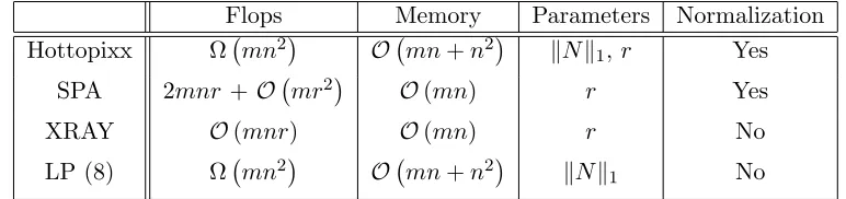
Table 1 gives the following information for the different algorithms: computational cost, memory requirement, parameters and if column normalization of the input matrix is necessary.
Flops Memory Parameters Normalization
Hottopixx Ω mn2
O mn+n2
kNk1,r Yes
SPA 2mnr+O mr2 O(mn) r Yes
XRAY O(mnr) O(mn) r No
LP (8) Ω mn2 O mn+n2 kNk1 No
Table 1: Comparison of robust algorithms for near-separable NMF for a densem-by-ninput matrix.
The LP have been solved using the IBM ILOG CPLEX Optimizer2 on a standard Linux
box. Because of the greater complexity of the LP-based approaches (formulating (2) and (8) as LP’s requires n2 +mn variables), the size of the input data matrices allowed on a standard machine is limited, roughlymn2∼106 (for example, on a two-core machine with 2.99GHz and 2GB of RAM, it already takes about one minute to process a 100-by-100 matrix using CPLEX). In this paper, we mainly focus on the robustness performance of the different algorithms and first compare them on synthetic data sets. We also compare them on the popular swimmer data set. Comparison on large-scale real-world data sets would require dedicated implementations, such as the parallel first-order method proposed by Bittorf et al. (2012) for the LP (2), and is a topic for further research. The code for all algorithms is available at https://sites.google.com/site/nicolasgillis/code.
2. The code is available for free for academia at http://www-01.ibm.com/software/integration/
5.3 Synthetic Data Sets
With the algorithms above we have run a benchmark with certain synthetic data sets particularly suited to investigate the robustness behaviour under influence of noise. In all experiments the problem dimensions are fixed to m = 50, n = 100 and r = 10. We conducted our experiments with six different data models. As we will describe next, the models differ in the way the factorH is constructed and the sparsity of the noise matrixN. Given a desired noise level , the noisy r-separable matrix ˜M = M +N = W H +N is generated as follows:
The entries ofW are drawn uniformly at random from the interval [0,1] (using Matlab’s
rand function). Then each column ofW is normalized so that its entries sum to one. The first r columns ofH are always taken as the identity matrix to satisfy the separa-bility assumption. The remaining columns of H and the noise matrixN are generated in two different ways (similar to Gillis and Vavasis, 2014):
1. Dirichlet. The remaining 90 columns of H are generated according to a Dirichlet distribution whoser parameters are chosen uniformly in [0,1] (the Dirichlet distribu-tion generates vectors on the boundary of the unit simplex so thatkH(:, j)k1 = 1 for
allj). Each entry of the noise matrixN is generated following the normal distribution
N(0,1) (using therandnfunction of Matlab).
2. Middle Points. The r(r2−1) = 45 next columns of H resemble all possible equally weighted convex combinations of pairs from the r leading columns ofH. This means that the corresponding 45 columns of M are the middle points of pairs of columns of W. The trailing 45 columns of H are generated in the same way as above, using the Dirichlet distribution. No noise is added to the first r columns of M, that is,
N(:,1 : r) = 0, while all the other columns are moved toward the exterior of the convex hull of the columns ofW using
N(:, j) =M(:, j)−w,¯ forr+ 1≤j≤n,
where ¯wis the average of the columns ofW (geometrically, this is the vertex centroid of the convex hull of the columns of W).
We combine these two choices forH andN with three options that control the pattern density ofN, thus yielding a total of six different data models:
1. Dense noise. Leave the matrixN untouched.
2. Sparse noise. Apply a mask toN such that roughly 75% of the entries are set to zero (using thedensity parameter of Matlab’s sprandfunction).
3. Pointwise noise. Keep only one randomly picked non-zero entry in each nonzero column of N.
5.3.1 Error Measures and Methodology
LetK be the set of indices extracted by an algorithm. In our comparisons, we will use the following two error measures:
• Index recovery: percentage of correctly extracted indices in K (recall that we know the indices corresponding to the columns of W).
• `1 residual norm: We measure the relative`1 residual by
1−min H≥0
kM˜ −M˜(:,K)Hks
kM˜ks
. (9)
Note that both measures are between zero and one, one being the best possible value, zero the worst.
The aim of the experiments is to display the robustness of the algorithms from Section 5.2 applied to the data sets described in the previous section under increasing noise levels. For each data model, we ran all the algorithms on the same randomly generated data on a predefined range of noise levels . For each such noise level, 25 data sets were generated and the two measures are averaged over this sample for each algorithm.
5.3.2 Results
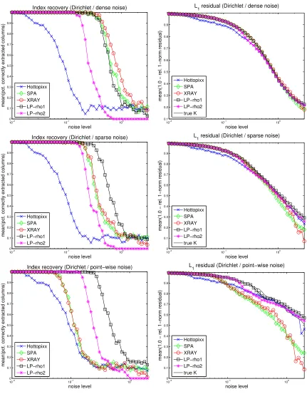
Figures 1 and 2 display the results for the three experiments of “Dirichlet” and “Middle Points” types respectively. For comparison purpose, we also display the value of (9) for the true column indices K of W inM, labeled “true K” in the plots. In all experiments, we observe that
• The new LP model (8) is significantly more robust to noise than Hottopixx, which confirms our theoretical results; see Section 2.1.
• The variant of LP (8) with ρ= 2 is less robust than with ρ= 1, as suggested by our theoretical findings from Section 2.1.
• SPA and XRAY perform, in average, very similarly.
Comparing the three best algorithms (that is, SPA, XRAY and LP (8) withρ= 1), we have that
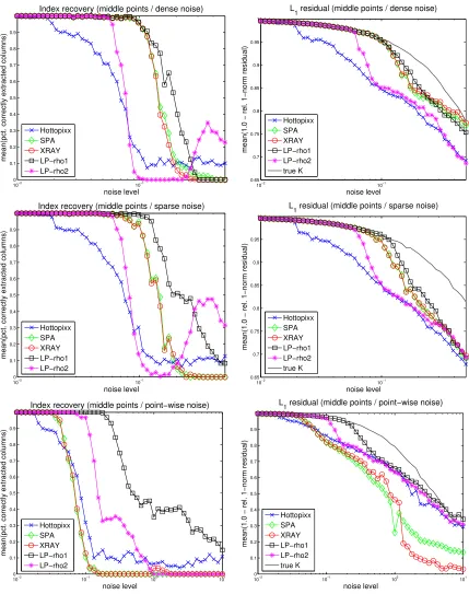
• In case of “dense” noise, they give comparable results; although LP (8) with ρ = 1 performs slightly worse for the “Dirichlet” type, and slightly better for the “Middle Points” type.
• In case of “sparse” noise, LP (8) with ρ = 1 performs consistently better then SPA and XRAY: for all noise levels, it identifies correctly more columns of W and the corresponding NMF’s have smaller `1 residual norms.
10−2 10−1 100 0 0.1 0.2 0.3 0.4 0.5 0.6 0.7 0.8 0.9 1 noise level
mean(pct. correctly extracted columns)
Index recovery (Dirichlet / dense noise)
Hottopixx SPA XRAY LP−rho1 LP−rho2 10−2 10−1 100 0.1 0.2 0.3 0.4 0.5 0.6 0.7 0.8 0.9 1 noise level
mean(1.0 − rel. 1−norm residual)
L
1 residual (Dirichlet / dense noise)
Hottopixx SPA XRAY LP−rho1 LP−rho2 true K 10−2 10−1 100 0 0.1 0.2 0.3 0.4 0.5 0.6 0.7 0.8 0.9 1 noise level
mean(pct. correctly extracted columns)
Index recovery (Dirichlet / sparse noise)
Hottopixx SPA XRAY LP−rho1 LP−rho2 10−2 10−1 100 0 0.1 0.2 0.3 0.4 0.5 0.6 0.7 0.8 0.9 1 noise level
mean(1.0 − rel. 1−norm residual)
L
1 residual (Dirichlet / sparse noise)
Hottopixx SPA XRAY LP−rho1 LP−rho2 true K 10−2 10−1 100 0 0.1 0.2 0.3 0.4 0.5 0.6 0.7 0.8 0.9 1 noise level
mean(pct. correctly extracted columns)
Index recovery (Dirichlet / point−wise noise)
Hottopixx SPA XRAY LP−rho1 LP−rho2 10−2 10−1 100 0 0.1 0.2 0.3 0.4 0.5 0.6 0.7 0.8 0.9 1 noise level
mean(1.0 − rel. 1−norm residual)
L
1 residual (Dirichlet / point−wise noise)
Hottopixx SPA XRAY LP−rho1 LP−rho2 true K
Figure 1: Comparison of near-separable NMF algorithms on “Dirichlet” type data sets. From left to right: index recovery and `1 residual. From top to bottom: dense
10−2 10−1 0 0.1 0.2 0.3 0.4 0.5 0.6 0.7 0.8 0.9 1 noise level
mean(pct. correctly extracted columns)
Index recovery (middle points / dense noise)
Hottopixx SPA XRAY LP−rho1 LP−rho2
10−2 10−1
0.65 0.7 0.75 0.8 0.85 0.9 0.95 1 noise level
mean(1.0 − rel. 1−norm residual)
L1 residual (middle points / dense noise)
Hottopixx SPA XRAY LP−rho1 LP−rho2 true K 10−2 10−1 0 0.1 0.2 0.3 0.4 0.5 0.6 0.7 0.8 0.9 1 noise level
mean(pct. correctly extracted columns)
Index recovery (middle points / sparse noise)
Hottopixx SPA XRAY LP−rho1 LP−rho2 10−2 10−1 0.65 0.7 0.75 0.8 0.85 0.9 0.95 1 noise level
mean(1.0 − rel. 1−norm residual)
L
1 residual (middle points / sparse noise)
Hottopixx SPA XRAY LP−rho1 LP−rho2 true K 10−2 10−1 100 101 0 0.1 0.2 0.3 0.4 0.5 0.6 0.7 0.8 0.9 1 noise level
mean(pct. correctly extracted columns)
Index recovery (middle points / point−wise noise)
Hottopixx SPA XRAY LP−rho1 LP−rho2 10−2 10−1 100 101 0 0.1 0.2 0.3 0.4 0.5 0.6 0.7 0.8 0.9 1 noise level
mean(1.0 − rel. 1−norm residual)
L
1 residual (middle points / point−wise noise)
Hottopixx SPA XRAY LP−rho1 LP−rho2 true K
Figure 2: Comparison of near-separable NMF algorithms on “Middle Points” type data sets. From left to right: index recovery and `1 residual. From top to bottom:
D/dense D/sparse D/pw MP/dense MP/sparse MP/pw
Hottopixx 2.5 2.5 3.6 4.4 4.3 4.2
SPA <0.1 <0.1 <0.1 <0.1 <0.1 <0.1 XRAY <0.1 <0.1 <0.1 <0.1 <0.1 <0.1
LP (8), ρ= 1 20.5 34.1 39.0 52.5 88.1 41.4
LP (8), ρ= 2 10.5 12.3 16.0 32.5 56.9 27.4
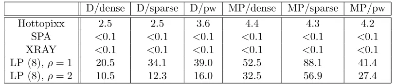
Table 2: Average computational time in seconds for the different algorithms and data mod-els. (D stands for Dirichlet, MP for middle points, pw for pointwise.)
W while SPA and XRAY can only extract a few for the “Dirichlet” type (performing as a guessing algorithm since they extract correctly only r/n= 10% of the columns of W), or none for the “Middle Points” type.
Note that LP (8) with ρ = 2 also performs consistently better then SPA and XRAY in case of “pointwise” noise.
Remark 13 For the “Middle Points” experiments and for large noise levels, the middle points of the columns of W become the vertices of the convex hull of the columns of M˜
(since they are perturbed toward the outside of the convex hull of the columns ofW). Hence, near-separable NMF algorithms should not extract any original column ofW. However, the index measure for LP (8)withρ= 2increases for larger noise level (although the`1 residual
measure decreases); see Figure 2. It is difficult to explain this behavior because the noise level is very high (close to 100%) hence the separability assumption is far from being satisfied and it is not clear what the LP (8) does.
Table 2 gives the average computational time for a single application of the algorithms to a data set. As expected, the LP-based methods are significantly slower than SPA and XRAY; designing faster solvers is definitely an important topic for further research. Note that the Hottopixx model can be solved about ten times faster on average than the LP model (8), despite the only essential difference being the trace constraint tr(X) = r. It is difficult to explain this behaviour as the number of simplex iterations or geometry of the central path cannot easily be set in relation to the presence or absence of a particular constraint.
Table 3 displays the index recovery robustness: For each algorithm and data model, the maximum noise level kNk1 for which the algorithm recovered on average at least 99% of
the indices corresponding to the columns of W. In all cases, the LP (8) with ρ = 1 is on par or better than all other algorithms.
5.4 Swimmer Data Set
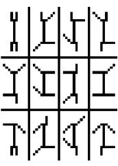
The swimmer data set is a widely used data set for benchmarking NMF algorithms (Donoho and Stodden, 2003). It consists of 256 binary images (20-by-11 pixels) of a body with four limbs which can be each in four different positions; see Figure 3. Let M ∈ {0,1}256×220
D/dense D/sparse D/pw MP/dense MP/sparse MP/pw
Hottopixx 0.014 0.018 0.016 0.016 0.018 0.015
SPA 0.220 0.154 0.052 0.077 0.071 0.032
XRAY 0.279 0.154 0.052 0.083 0.071 0.032
LP (8), ρ= 1 0.279 0.195 0.197 0.083 0.098 0.178
LP (8), ρ= 2 0.137 0.121 0.141 0.055 0.055 0.075
Table 3: Index recovery robustness: Largest noise level kNk1 for which an algorithm achieves almost perfect index recovery (that is, at least 99% on average).
Figure 3: Sample images of the swimmer data set.
column to a pixel. The matrixM is 16-separable: up to permutation,M has the following form
M = W
I16, I16, I16,
1
4E16×14,016×158
,
where Em×n denotes the m-by-n all-one matrix. In fact, all the limbs are disjoint and contain three pixels (hence each column of W is repeated three times), the body contains fourteen pixels and the remaining 158 background pixels do not contain any information.
Remark 14 (Uniqueness of H) Note that the weights 14E16×14 corresponding to the
pix-els belonging to the body are not unique. The reason is that the matrix W is not full rank (in fact, rank(W) = 13) implying that the convex hull of the columns of W and the origin is not a simplex (that is, r+ 1vertices in dimension r). Therefore, the convex combination needed to reconstruct a point in the interior of that convex hull is not unique (such as a pixel belonging to the body in this example); see the discussion in Gillis (2012).
Let us compare the different algorithms on this data set:
• SPA. Because the rank of the input matrixM is equal to thirteen, the residual matrix becomes equal to zero after thirteen steps and SPA cannot extract more than thirteen indices hence it fails to decomposeM.
any of them can be extracted. Since there are 48 pixels belonging to a limb and only 14 to the body, XRAY is more likely to extract a pixel on a limb (after which it is able to correctly decompose M). However, if the first pixel extracted by XRAY is a pixel of the body then XRAY requires to be run with r = 17 to achieve a perfect decomposition. Therefore, XRAY succeeds on this example only with probability
48
62 ∼ 77% (given that XRAY picks a column at random among the one maximizing
the criterion). We consider here a run where XRAY failed, otherwise it gives the same perfect decomposition as the new LP based approaches; see below.
• Hottopixx. With = 0 in the Hottopixx LP model (2), the columns of W are correctly identified and Hottopixx performs perfectly. However, as soon as exceeds approximately 0.03, Hottopixx fails in most cases. In particular, if p is chosen such that its smallest entry does not correspond to a columns of W, then it always fails (see also the discussion in Example 1). Even ifp is not chosen by an adversary but is randomly generated, this happens with high probability since most columns ofM do not correspond to a column ofW.
• LP (7) with ρ = 1. For up to approximately 0.97, the LP model (7) (that is, the new LP model based on relative error) idenfities correctly the columns ofW and decomposes M perfectly.
• LP (8) with ρ = 1. For up to approximately 60, (note that the `1 norm of the
columns ofW is equal to 64), the LP model (8) (that is, the new LP model based on absolute error) identifies correctly the columns ofW and decomposes M perfectly.
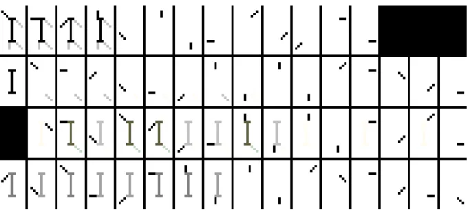
Figure 4 displays the optimal weights corresponding to the columns ofM extracted with the different algorithms (that is, the rows of the matrixH∗ = argminH≥0||M−M(:,K)H||F where K is the index set extracted by a given algorithm): the error for SPA is 20.8, for XRAY 12, for Hottopixx 12 and for the new LP models 0. Note that we used = 0.1 for Hottopixx and the new LP model (a situation in which Hottopixx fails in most cases; see the discussion above—for the particular run shown in Figure 4, Hottopixx extracts a background pixel corresponding to a zero column of M). Note also that we do not display the result for the LP (8) because it gave an optimal solution similar to that of the LP (7). Finally, it is interesting to point out that the nonnegative rank of M is equal to 16 hence the new LP models actually detect the nonnegative rank of M.
6. Conclusion and Further Work
In this paper, we have proposed a new more practical and more robust LP model for near-separable NMF which competes favorably with two state-of-the-art methods (outperforming them in some cases). It would be particularly interesting to investigate the following direc-tions of research:
Figure 4: Weights corresponding to the extracted indices by the different algorithms. From to to bottom: SPA, XRAY, Hottopixx ( = 0.1) and the new LP model (7) (= 0.1).
• Improvement of the theoretical bound on the noise level for Algorithm 3 to extract the right set of columns of the input data matrix in case duplicates and near duplicates are present in the data set (cf. Section 2.2).
• Design of practical and robust near-separable NMF algorithms. For example, would it be possible to design an algorithm as robust as our LP-based approach but compu-tationally more effective (e.g., running inO(mnr) operations)?
Acknowledgments
The authors would like to thank the reviewers for their feedback which helped improve the paper.
Appendix A. Proof of Theorem 2
The next two lemmas are simple generalizations of Lemmas 2 & 3 in Gillis (2013). Given any feasible solution X of the the linear program (3), the first one shows that the`1 norm
of the error M −M X with respect to the original noiseless data matrix is proportional to , that is, kM˜ −M X˜ k1 ≤ O(). The second one proves that the diagonal entries ofX
corresponding to the columns of W must be larger than 1− O().
Lemma 15 Suppose M˜ =M +N where kM(:, j)k1 = 1 for all j and kNk1 ≤ <1, and
suppose X is a feasible solution of (3). Then,
kXk1 ≤1 +
ρ+ 2 1−
and kM−M Xk1 ≤
ρ+ 2 1−
Proof First note that kM˜k1 ≤ kMk1 +kNk1 ≤ 1 + and kM Xk1 = kXk1. By the feasibility of X for (3),
ρ≥ kM˜ −M X˜ k1 ≥ kM X˜ k1− kM˜k1 ≥ kM Xk1− kN Xk1−(1 +)≥ kXk1−kXk1−1−,
hencekXk1≤1 +1ρ+2−, implying thatkN Xk1 ≤ kNk1kXk1 ≤1 +(ρ1+2)−. Therefore
ρ≥ kM˜ −M X˜ k1 =kM+N−(M+N)Xk1 ≥ kM−M Xk1−−
1 +(ρ+ 2) 1−
,
from which we obtainkM−M Xk1 ≤
ρ+ 2 + (ρ1+2)−
=
ρ+2 1−
Lemma 16 Let M˜ = M +N where ||M(:, j)||1 = 1 for all j, admits a rank-r separable
factorizationW H withW κ-robustly conical and||N||1 ≤ <1, and has the form (1)with
maxi,jHij0 ≤β <1 and W, H≥0. Let also X be any feasible solution of (3), then
X(j, j)≥1− 2
κ(1−β)
ρ+ 2 1−
for all j such that M(:, j) =W(:, k) for some 1≤k≤r.
Proof The idea of the proof is the following: by assumption, each column of W is isolated from the convex hull of the other columns of M. Therefore, to being able to approximate it up to errorO(), its corresponding diagonal entry must be large enough.
Let K be the set of r indices such that M(:,K) =W. Let also 1≤ k ≤r and denote
j=K(k) so thatM(:, j) =W(:, k). By Lemma 15,
||W(:, k)−W HX(:, j)||1≤
ρ+ 2 1−
. (10)
Since H(k, j) = 1,
W HX(:, j) =W(:, k)H(k,:)X(:, j) +W(:,R)H(R,:)X(:, j)
=W(:, k)X(j, j) +H(k,J)X(J, j)+W(:,R)y,
whereR={1,2, . . . , r}\{k},J ={1,2, . . . , n}\{j} andy =H(R,:)X(:, j)≥0. We have
η=X(j, j) +H(k,J)X(J, j)≤X(j, j) +β
1 +(ρ+ 2)
1− −X(j, j)
, (11)
since||H(k,J)||∞≤β and ||X(:, j)||1 ≤1 +(ρ1+2)− (Lemma 15). Hence
||W(:, k)−W HX(:, j)||1≥(1−η)
W(:, k)−W(:,R) y 1−η
1
Combining Equations (10), (11) and (12), we obtain
1−
X(j, j) +β
1 +(ρ+ 2)
1− −X(j, j)
≤
κ
ρ+ 2 1−
which gives, using the fact thatκ, β ≤1,
X(j, j)≥1− 2
κ(1−β)
ρ+ 2 1−
.
If the diagonal entries corresponding to the columns of W of a feasible solution X of (3) are large, then the other diagonal entries will be small. In fact, the columns of M are contained in the convex hull of the columns of W hence can be well approximated with convex combinations of these columns.
Lemma 17 Let M˜ = M +N where ||M(:, j)||1 = 1 for all j, admits a rank-r separable
factorization W H and ||N||1 ≤ , and has the form (1). Let K be the index set with r
elements such that M(:,K) =W. Let also X∗ be an optimal solution of (3)such that
X∗(k, k)≥γ for all k∈ K, (13)
where 0≤γ ≤1. Then,
X∗(j, j)≤1−minγ,ρ
2
for allj /∈ K.
Proof Let X be any feasible solution of (3) satisfying (13), and α = min γ,ρ2
. Let us show that thejth column of X for somej /∈ K can be modified as follows
X(i, j)←
1−α ifi=j, αH(i, j) ifi∈ K,
0 otherwise,
while keeping feasibility. First, αH(i, j) ≤ γ ≤ X(i, i) for all i ∈ K hence the condition
X(i, j) ≤ X(i, i) for all i, j is satisfied while, clearly, 0 ≤ X(i, i) ≤1 for all i. It remains to show that ||M˜(:, j)−M X˜ (:, j)||1≤ ρ. By assumption, M(:, j) =W H(:, j) = αW H(: , j) + (1−α)M(:, j) hence
˜
M(:, j) =α(M(:, j) +N(:, j)) + (1−α) ˜M(:, j)
=α(W H(:, j) +N(:, j)) + (1−α) ˜M(:, j).
This gives
||M˜(:, j)−M X˜ (:, j)||1 =α||M(:, j) +N(:, j)−(W +N(:,K))H(:, j)||1≤2α≤ρ,
since the columns of H sum to one, and ||N||1 ≤ . This result implies that any optimal
jth column of X∗ using the construction above and obtain a strictly better solution since the vectorp in the objective function only has positive entries.
We can now combine Lemmas 16 and 17 to prove robustness of Algorithm 2 when there are no duplicates nor near duplicates of the columns of W in the data set.
Proof [Proof of Theorem 2] Let X be an optimal solution of (3). Let us first consider the case = 0, which is particular because it allows duplicates of the columns of W in the data set and the value of ρ does not influence the analysis since ρ= 0 for anyρ >0. Let denote
Kk={j |M(:, j) =W(:, k)},
the set of indices whose corresponding column of M is equal to the kth column ofW. By assumption, κ > 0 hence for all 1 ≤ k ≤ r we have W(:, k) ∈/ cone(W(:,K¯)) where ¯K =
{1,2, . . . , r}\{k}. This implies thatP
j∈KkX(j, j)≥1 for allk. Since we are minimizing a
positive linear combination of the diagonal entries ofXand assigning a weight of one to each cluster Kk is feasible (see Equation 1), we have P
j∈KkX(j, j) = 1. Moreover, assigning all
the weight to the index inKkwith the smallest entry in pminimizes the objective function (and this index is unique since the entries of p are distinct). Finally, for all 1 ≤ k ≤ r, there exists a unique j such that M(:, j) =W(:, k) and X(j, j) = 1 which gives the result for= 0.
Otherwise > 0 andβ < 1, and the result follows from Lemmas 16 and 17: LetK be the set ofr indices such thatM(:,K) =W. By Lemma 16, we have
X(k, k)≥1− 2
κ(1−β)
ρ+ 2 1−
, for all k∈ K,
while, by Lemma 17,
X(j, j)≤max
1− ρ
2, 2 κ(1−β)
ρ+ 2 1−
, for all j /∈ K.
Therefore, if
1− 2
κ(1−β)
ρ+ 2 1−
> f ≥ max
1−ρ
2, 2 κ(1−β)
ρ+ 2 1−
,
where f = 1− min(12 ,ρ) = max 12,1−ρ2
, then Algorithm 2 extracts the r indices corre-sponding to the columns ofW. The above conditions are satisfied if
2 κ(1−β)
ρ+ 2 1−
< ρ
2 and
2 κ(1−β)
ρ+ 2 1−
< 1
2,
that is, 1− < κ(1−4(β) min(1ρ+2) ,ρ). Taking
≤ κ(1−β) min(1, ρ)
5(ρ+ 2) <
κ(1−β) min(1, ρ)
ρ+ 2
1−
4
gives the results since≤ 1 5(ρ+2) <
1
10 for any ρ >0 hence 1−
Appendix B. Proof of Theorem 6
Theorem 6 can be proved using a particular construction.
Proof [Proof of Theorem 6] Let us consider
W =
κ
2Ir
(1−κ2)eTr
, H =
Ir βIr+ 1−β r−1(ere
T r −Ir)
, and N = 0,
where er ∈ Rr is the all-ones vector, 1r ≤ β < 1 and W is κ-robustly conical with κ > 0 (Gillis, 2013). Definep= Ker
er
for some large constantK constant. The matrix
X =
1−κ(1ρ−β)Ir 0 ρ
κ(1−β)Ir Ir
!
is a feasible solution of (3) for any≤ κ(1ρ−β). In fact, for all 1≤j≤r,
||M(:, j)−M X(:, j)||1= ρ
κ(1−β)||M(:, j)−M(:, j+r)||1 =ρ,
and it can be easily checked that X satisfies the other constraints. By Lemma 7 of Gillis (2013), for K sufficiently large, any optimal solutionX∗ of (3) must satisfy
min
1≤k≤rX
∗
(k, k)≤ max
1≤k≤rX(k, k) = 1−
ρ κ(1−β),
(otherwisepT diag(X∗)> pTdiag(X) forK sufficiently large). For the columns of W to be extracted, one requiresX∗(k, k)>1−min(12 ,ρ) for all 1≤k≤r hence it is necessary that
1− ρ
κ(1−β) >1−
min(1, ρ)
2 ⇐⇒ <
κ(1−β) 2
min(1, ρ)
ρ ,
for Algorithm 2 to extract the firstr columns ofM.
Appendix C. Proof of Theorem 7
Proof [Proof of Theorem 7] The matrix X0 from Equation (1) is a feasible solution of (3); in fact,
||M˜ −M X˜ 0||1=||M+N −(M+N)X0||1≤ ||M−M X0||1+||N||1+||N X0||1 ≤2,
since M = M X0, ||N||1 ≤ and ||N X0||1 ≤ ||N||1||X0||1 ≤ as ||X0||1 = 1. Therefore,
sincep=e, any optimal solution X∗ of (3) satisfies
tr(X∗) =pTdiag(X∗)≤pT diag(X0) =r.
be distinct and only the condition tr(X) ≤ r is necessary. Note that Theorem 5 in Gillis (2013) guarantees that there are r disjoint clusters of columns of ˜M around each column of W whose weight is strictly larger r+1r . Therefore, the total weight is strictly larger than
r− r
r+1 > r−1 while it is at mostr(since tr(X
∗)≤r) implying thatr=lPn
i=1X∗(i, i)
m .
Appendix D. Proof of Theorem 9
The proof of Theorem 9 works as follows: Let X be a feasible solution of (3). First, we show that the diagonal entries of X corresponding to the columns of W and T must be large enough (this follows from Theorem 2). Second, we show that the`1 norm of the rows
of X corresponding to the columns of W (resp. T) must be sufficiently large (resp. low) because the columns ofW (resp.T) must be used (resp. cannot be used) to reconstruct the other columns ofM.
Proof [Proof of Theorem 9] In case β = 1, = 0 and the proof is similar to that of Theorem 2; the only difference is that the condition from Equation (5) has to be used to show that no weight can be assigned to off-diagonal entries of the rows of an optimal solution of (3) corresponding to the columns ofT. Otherwise β <1 and there are no duplicate nor near duplicate of the columns of W in the data set.
Let assume without loss of generality that ˜M has the form
˜
M = [T, W, W H0] +N,
that is, the first tcolumns correspond to T and the r next ones toW. Let then X be an optimal solution of (3).
Since [W, T] is κ-robustly conical, Theorem 2 applies (as if the columns of T were not outliers) and, for all 1≤k≤r+t,
X(k, k)≥1− 8
κ(1−β)(1−) ≥ 1 2,
while X(j, j) ≤ 8
κ(1−β)(1−) ≤ 1
2 for all j > r+t, since ≤
ν(1−β)
20(n−1) whereν = min(κ, η, δ).
Therefore, only the firstr+tindices can potentially be extracted by Algorithm 5. It remains to bound above (resp. below) the off-diagonal entries of the rows of X corresponding toT
(resp. W).
By Lemma 16 (see also Gillis, 2013, Lemma 2), we have for all 1≤j≤n
||M(:, j)−M X(:, j)||1 ≤ 4
1− and ||X(:, j)||1≤1 +
4
1−.
Using the fact that [W, T] isκ-robustly conical, for all 1≤k≤t, we have
||T(:, k)−M X(:, k)||1≥(1−X(k, k)) min
x≥0,y≥0||T(:, k)−T(:,
¯
K)x−W y||1 ≥(1−X(k, k))κ,
implying that for all 1≤k≤t
X(k, k)≥1− 4
since 1−4 ≤5 because≤ 1
20. Therefore,
X
j6=k
X(j, k)≤ ||X(:, k)||1−X(k, k)≤
4
1−+
4 κ(1−) ≤
8 κ(1−),
asκ, ≤1. Let t+ 1≤j ≤nand 1≤k≤t, we have
||M(:, j)−M X(:, j)||1 ≥min
x miny≥0||T(:, k) +T(:,
¯
K)y−W x||1 ≥ηX(k, j),
see Equation (5), which impliesX(k, j)≤ η(14−). Hence, for all 1≤k≤t, we have X
j6=k
X(k, j)≤(t−1) 8
κ(1−) + (n−r−t) 4 η(1−) ≤
8(n−1) ν(1−) ≤
1 2.
since ν = min(κ, η, δ). By assumption, for each t+ 1 ≤ k ≤ t+r, there exists some j
satisfying M(:, j) =W H(:, j)6=W(:, k) and
min
x≥0||M(:, j)−W(:,
¯
K)x||1 ≥δ, where ¯K={1,2, . . . , r}\{k},
see Equation (6). For t+r < j ≤ n, we have X(j, j) ≤ κ(1−β8)(1−). Let us denote
µ= κ8((1n−−βr)(1−t−)) which is an upper bound for the total weight that can be assigned to the columns ofM different from W and T. Then, using Equation (6), we have
kM(:, j)−M X(:, j)k1 ≥(1−µ) min y≥0
M(:, j)− 1
1−µW X(t+ 1:r+t, j)−T y
1 ≥(1−µ)
1−X(k, j)
1−µ
δ.
This implies
X(k, j) 1−µ ≥1−
4 δ(1−µ)(1−) and
X(k, j)≥1− 8(n−r−t)
κ(1−β)(1−) − 4 δ(1−)
≥1− 8(n−1)
ν(1−β)(1−) ≥ 1 2,
sinceβ ≤1 and≤ 20(ν(1n−−β1)), and the proof is complete.
References
S. Arora, R. Ge, R. Kannan, and A. Moitra. Computing a nonnegative matrix factorization – provably. In Proc. of the 44th Symp. on Theory of Computing, STOC ’12, pages 145– 162, 2012a.
S. Arora, R. Ge, and A. Moitra. Learning topic models - going beyond SVD. InProc. of the 53rd Annual IEEE Symp. on Foundations of Computer Science, FOCS ’12, pages 1–10, 2012b.
J.M. Bioucas-Dias, A. Plaza, N. Dobigeon, M. Parente, Q. Du, P. Gader, and J. Chanussot. Hyperspectral unmixing overview: Geometrical, statistical, and sparse regression-based approaches. IEEE Journal of Selected Topics in Applied Earth Observations and Remote Sensing, 5(2):354–379, Apr. 2012.
V. Bittorf, B. Recht, E. R´e, and J.A. Tropp. Factoring nonnegative matrices with linear programs. In Advances in Neural Information Processing Systems (NIPS ’12), pages 1223–1231, 2012.
T.-H. Chan, W.-K. Ma, C.-Y. Chi, and Y. Wang. A convex analysis framework for blind separation of non-negative sources. IEEE Trans. on Signal Processing, 56(10):5120–5134, 2008.
L. Chen, P.L. Choyke, T.-H. Chan, C.-Y. Chi, G. Wang, and Y. Wang. Tissue-specific compartmental analysis for dynamic contrast-enhanced MR imaging of complex tumors. IEEE Trans. on Medical Imaging, 30(12):2044–2058, 2011.
D. Donoho and V. Stodden. When does non-negative matrix factorization give a cor-rect decomposition into parts? In Advances in Neural Information Processing Systems (NIPS ’03), 2003.
E. Elhamifar, G. Sapiro, and R. Vidal. See all by looking at a few: Sparse modeling for find-ing representative objects. In IEEE Conf. on Computer Vision and Pattern Recognition, 2012.
E. Esser, M. Moller, S. Osher, G. Sapiro, and J. Xin. A convex model for nonnegative matrix factorization and dimensionality reduction on physical space. IEEE Trans. on Image Processing, 21(7):3239–3252, 2012.
N. Gillis. Sparse and unique nonnegative matrix factorization through data preprocessing. Journal of Machine Learning Research, 13(Nov):3349–3386, 2012.
N. Gillis. Robustness analysis of Hottopixx, a linear programming model for factoring nonnegative matrices. SIAM J. Mat. Anal. Appl., 34(3):1189–1212, 2013.
N. Gillis and S.A. Vavasis. Fast and robust recursive algorithms for separable nonnegative matrix factorization. IEEE Trans. Pattern Anal. Mach. Intell., 36(4):698–714, 2014.
A. Kumar, V. Sindhwani, and P. Kambadur. Fast conical hull algorithms for near-separable non-negative matrix factorization. In Int. Conf. on Machine Learning (ICML ’13), vol-ume 28, pages 231–239. 2013.