Geometric Variance Reduction in Markov Chains: Application to Value Function and Gradient Estimation

Geometric Variance Reduction in Markov Chains:

Application to Value Function and Gradient Estimation

Rémi Munos [email protected]

Centre de Mathématiques Appliquées Ecole Polytechnique

91128 Palaiseau, France

Editor: Shie Mannor

Abstract

We study a variance reduction technique for Monte Carlo estimation of functionals in Markov chains. The method is based on designing sequential control variates using successive approxi-mations of the function of interest V . Regular Monte Carlo estimates have a variance of O(1/N), where N is the number of sample trajectories of the Markov chain. Here, we obtain a geometric variance reduction O(ρN_{)(withρ<1) up to a threshold that depends on the approximation error} V−AV , whereAis an approximation operator linear in the values. Thus, if V belongs to the right approximation space (i.e.AV=V ), the variance decreases geometrically to zero.

An immediate application is value function estimation in Markov chains, which may be used for policy evaluation in a policy iteration algorithm for solving Markov Decision Processes.

Another important domain, for which variance reduction is highly needed, is gradient estima-tion, that is computing the sensitivity ∂αV of the performance measure V with respect to some parameterαof the transition probabilities. For example, in policy parametric optimization, com-puting an estimate of the policy gradient is required to perform a gradient optimization method.

We show that, using two approximations for the value function and the gradient, a geometric variance reduction is also achieved, up to a threshold that depends on the approximation errors of both of those representations.

1. Introduction

We consider a Markov chain over a finite state space

X

_{defined by the transition matrix P. Note that}

although we consider a finite state space for simplicity, this work can be easily extended to the case of infinite state spaces (countable or continuous). Write X(x)a trajectory(xt)t≥0starting at a state

x0=x. LetΨ(r,X(x))be a functional that depends on some function r :

X

→IR and the trajectory

X(x), and write V(x)the expectation of the functional that we wish to evaluate:

V(x) =E[Ψ(r,X(x))]. (1)

Here, the quantity of interest V is expressed in terms of a probabilistic representation, as an expectation of a functional that depends on trajectories. We will consider a functionalΨ(r,·)that is linear in r, and such that its expectation V may equivalently be expressed in terms of a solution to

a linear system

L

_{V =r, (2)}

Such an example ofΨis the sum of discounted rewards r received along the trajectory:

Ψ(r,X(x)) =

∑

t≥0

γt_r(x

t). (3)

with 0<γ<1 being a discount factor. In that case, V is the solution to the Bellman equation (2) with

L

_=I−γ_{P. Indeed, using matrix notations, V=}∑_t≥0γt_Pt_{r= (I−}γ_P)−1_r.

A regular Monte-Carlo (MC) method would estimate V(x) by sampling N independent trajec-tories{Xn(x)}1≤n≤N starting from x and calculate the average _N1∑nN=1Ψ(r,Xn(x)). The variance of

such an estimator is of order 1/N. Variance reduction is crucial since the numerical approximation

error of the quantity of interest is directly related to the variance of its estimate.

Variance reduction techniques include importance sampling, correlated sampling, control vari-ates, antithetic variates and stratified sampling, see e.g. (Hammersley and Handscomb, 1964; Hal-ton, 1970). Geometric variance reduction rates have been obtained by processing these variance reduction methods iteratively, the so-called sequential (or recursive) Monte-Carlo. Examples in-clude adaptive importance sampling (Kollman et al., 1999) and what Halton called the “Third Se-quential Method” (Halton, 1994) based on seSe-quential correlated sampling and control variates. This approach has been recently developed in (Maire, 2003) for numerical integration and, more related to our work, applied to (continuous time) Markov processes in (Gobet and Maire, 2005).

The idea is to replace the expectation of Ψ(r,·) by the expectation ofΨ(r−

L

_{W,·) for some}

function W close to V . From the linearity ofΨand the equivalence between the representations (1) and (2), for any W , one has

V(x) =W(x) +E[Ψ(r−

L

_W,X(x))].

Thus, if W is a good approximation of V , the residual r−

L

_{W is small, and the variance is low.}

In the sequential method described in this paper, we use successive approximations Vnof V to

estimate by Monte Carlo a correction Enusing the residual r−

L

VninΨ, which is used to process

a new approximation Vn+1. We consider an approximation operator

A

that is linear in the values.

We show that (for enough sample trajectories at each iteration) the variance of the estimator has a geometric rateρN(withρ<1, and N the total number of sampled trajectories) until some threshold is reached, whose value is related to the approximation error

A

_{V−V .}

An interesting extension of this idea concerns the estimation of the gradient∂_αV of V with

re-spect to (w.r.t.) some parameterαof the transition matrix P. A useful application of such sensitivity analysis appears in policy gradient estimation. An optimal control problem may be approximated by a parametric optimization problem in a given space of parameterized policies. Thus, the transi-tion matrix P depends on some (possible multidimensional) policy parameterα. In order to apply gradient methods to search for a local maximum of the performance in the parameter space, one wishes to estimate the policy gradient, i.e. the sensitivity Z =∂_αV of the performance measure

with respect toα. The gradient may be expressed as an expectation Z(x) =_E[Φ(r,X(x))], using the so-called likelihood ratio or score method (Reiman and Weiss, 1986; Glynn, 1987; Williams, 1992; Baxter and Bartlett, 2001; Marbach and Tsitsiklis, 2003). The gradient Z is also the solution to a linear system

L

_Z=−∂_α

L L

−1_r=−∂_α

L

_{V. (4)}

(note that the derivative operator∂αonly applies to

L

_{). Indeed, since V solves V =}

L

−1_{r, we have}

L

_=I−γ_{P, thus}∂_α

L

₌₋γ∂_{αP and}

Z=γ(I−γP)−1∂_αP(I−γP)−1r=

∑

t≥0

γt+1_Pt_∂

αP

∑

s≥0

γs_Ps_r.

The functionalΦmay thus be defined as

Φ(r,X(x)) =

∑

t≥0

γt+1∂αP(xt,xt+1)

P(xt,xt+1) _s≥0

∑

γ

s_r(x

s+t+1), (5)

which may be rewritten as

Φ(r,X(x)) =

∑

t≥0

γt_r(x t)

t−1

∑

s=0

∂αP(xs,xs+1)

P(xs,xs+1) .

We show that, using two approximations Vn and Zn of the value function and the gradient, a

geometric variance reduction is also achieved, up to a threshold that depends on the approximation errors of both of those representations.

Numerical experiments on a simple Gambler’s ruin problem illustrate the approach.

2. Value Function Estimation

We first describe the approximation operator linear in the values considered here, then describe the algorithm, and state the main result on geometric variance reduction.

2.1 Approximation Operator

A

We consider a fixed set of J representative states

X

_{J :={xj ∈}

X

_{}1≤j≤J and basis functions{}φ_j:

X

_{→IR}1≤j≤J. The linear approximation operator}

A

_{maps any function W :}

X

_{J→IR to the function}

A

_{W :}

X

_{→IR, according to}

A

_{W(x) =}

J

∑

j=1

W(xj)φj(x). (6)

With a slight abuse of notation, for any function W :

X

_{→IR, we define}

A

_{W :}

X

_{→IR similarly}

from the values of W at

X

_{J. This kind of function approximation includes:}

• Linear approximation, for example with Spline, Polynomial, Radial Basis, Fourier or Wavelet

decomposition.

A

_{W is the projection of a function W onto the space spanned by a set of}

func-tions{ψk:

X

→IR}1≤k≤K, i.e. the function minimizing some norm (induced by a discrete

inner producthf,gi:=∑J

j=1µjf(xj)g(xj), for some distribution µ over

X

J):

min

α∈IRK

K

∑

k=1

αkψk−W

2.

The solutionα solves the linear system Aα=b with A an K×K-matrix of elements Akl= hψk,ψliand b a K-vector of components bk=hW,ψki. Thusαk=∑Kl=1A−1kl ∑Jj=1µjψl(xj)W(xj)

and the best fit∑K_k=1αkψkis thus of type (6) with

φj(x) =µj K

∑

k=1 K

∑

l=1

• Non-parametric approximation, such as k-nearest neighbors (whereφj(x) = 1_k if x has xj

as one of its k−nearest neighbors, andφj(x) =0 otherwise), locally weighted learning and

Kernel regression (Atkeson et al., 1997; Hastie et al., 2001), where functions similar to (7)

may be derived (with the matrix A being dependent on x through the kernel), and Support

Vector Regression (when using a quadratic loss function) (Vapnik et al., 1997; Vapnik, 1998).

2.2 The Algorithm

We assume the equivalence between the probabilistic interpretation (1) and the representation as solution to the linear system (2), i.e. for any function f :

X

_→IR,

f(x) =E[Ψ(

L

_{f,X(x))]. (8)}

We consider successive approximations Vn∈IRJof V defined at the states

X

J= (xj)1≤j≤J

recur-sively:

• We initialize V0(xj) =0.

• At stage n, we use the values Vn(xj) to provide a new estimate of V(xj). Let En(xj) :=

V(xj)−

A

Vn(xj) be the approximation error at the states (xj)1≤j≤J. From the equivalence

property (8), we have:

A

_{Vn(x) =E[}Ψ₍

L A

_{Vn,X(x))]. Thus, by linearity of}Ψ _{w.r.t. its first}

variable,

En(xj) =E[Ψ(r−

L A

Vn,X(xj))].

Now, we use a Monte Carlo technique to estimate En(xj)at each representative state xj, using

M trajectories(Xn,m(xj))1≤m≤M: we calculate the average

c

En(xj):= 1

M

M

∑

m=1

Ψ(r−

L A

_Vn,Xn,m_(xj)),

and define the new approximation at the states

X

_J:

Vn+1(xj):=

A

Vn(xj) +cEn(xj). (9) Remark 1 Notice that there is a slight difference between this algorithm and that of (Gobet and

Maire, 2005), which may be written

Vn+1(xj) =Vn(xj) +

A

h₁

M

M

∑

m=1

Ψ(r−

L

_Vn,Xn,m_(xj))i_.

Our formulation enables us to avoid the assumption of the idempotent property for

A

_{(i.e. that}

A

2₌

_A

_{) which does not hold in general in non-parametric approximation (e.g. in k-nearest}

neigh-bors, for k≥2) and guarantees that Vnis an unbiased estimate of V , for all n, as showed in the next

paragraph.

2.3 Properties of the Estimates Vn

We write the conditional expectations and variances:

En[Y] =E[Y|Xp,m(xj),0≤p<n,1≤m≤M,1≤ j≤J]

Expectation of Vn. From the definition (9),

En[Vn+1(xj)] =

A

Vn(xj) +En(xj) =V(xj).

ThusE[Vn(xj)] =V(xj)for all n≥1: the approximation Vn(xj)is an unbiased estimate of V(xj).

Variance of Vn. Write vn=sup1≤j≤JVar Vn(xj). The following result (whose proof is provided

in Appendix A) expresses that for large enough values of M, the variance decreases geometrically with n.

Theorem 2 We have

vn+1≤ρMvn+

2

M

V

Ψ(V−

A

V) (10)

withρM=_M2 ∑Jj=1

p

V

_Ψ(φ_j)2_{, using the notation}

V

_{Ψ(f):= sup}

1≤j≤J

VarΨ(

L

_f,X(xj)).

Thus, for large enough values of M, (i.e. wheneverρM<1),(vn)n decreases geometrically at rate

ρM, up to the threshold

lim sup

n→∞ vn≤

1 1−ρM

2

M

V

Ψ(V−

A

V).

If V belongs to the space of functions that are representable by

A

_{, i.e.}

A

_{V =V , then the}

variance geometrically decreases to 0 at rate ρN with ρ:=ρ1_M/M and N being the total number of sample trajectories per state xj(i.e. N is the product of the number n of iterations by the number M

of trajectories per iteration and state xj).

Notice that the threshold depends on the variance ofΨfor the function

L

_(V−

A

_{V) =r−}

L A

_{V ,}

the residual of the representation (by

A

_{) of V . Notice also that this threshold depends on V−}

A

_{V only at states reached by the trajectories {X(xj)}x}

j∈XJ: a uniform (over the whole domain)

representation of V is not required.

Of course, once the threshold is reached, a further convergence of O(1/N) can be obtained thereafter, using regular Monte Carlo.

2.4 Example: The Infinite Horizon, Discounted Case

Let us illustrate the sequential control variates algorithm to value function estimation in Markov chains in the infinite horizon, discounted case (3). The value function

V(x) =E

∑

t≥0

γt_r(x t)

solves Bellman’s equation: V =r+γPV , which may be written as the linear system (2) with

L

₌ I−γP.

In the previous algorithm, at stage n, the approximation error En(xj) =V(xj)−

A

_Vn(xj)is

there-fore the expectation

En(xj) =E

∑

t≥0

γt_[r(x

t)−

A

Vn(xt) +γP

A

Vn(xt)]|x0=xj

We notice that the term r−

A

_Vn+γ_P

A

_{Vnis the Bellman residual of the approximation}

A

_{Vn. The}

estimate thus has zero variance if this approximation happens to be the value function. Following the algorithm, the next approximation Vn+1is defined by (9) withcEn(xj)being a Monte Carlo estimate

of (11).

Remark 3 Note that the expectation operator P may not be easy to process. In model-free learning,

it would be interesting to replace the term P

A

_Vn(xt)by

A

_{Vn(xt+1)in (11) leaving the expectation} unchanged. However, this would introduce some additional variance that annihilates the benefit of the technique.

Nevertheless, the term P

A

_{Vnmay actually be computed as}

A

0_{Vn, where}

A

0_{is an approximation} operator defined by another set of basis functions{φ0

j:=Pφj}1≤j≤J(i.e.φ0j(x):=∑y∈XP(x,y)φj(y),

1≤ j≤J). Indeed, for any W :

X

_J→IR,

P

A

_{W(x) =}

∑

y∈X

P(x,y) J

∑

j=1

W(xj)φj(y) = J

∑

j=1

W(xj)φ0j(x) =

A

0W(x).

These functions{φ0

j:=Pφj}1≤j≤Jmay be precomputed before simulations, or approximated on-line

with function approximation techniques.

2.5 Other Examples

Other possible settings include the finite-horizon time, the infinite horizon stochastic shortest path, and average reward problems, briefly described now.

In a finite-time horizon problem, the value V(t,x)is time-dependent. So let X(t,x) ={xs}t≤s≤T

be a trajectory starting from x∈

X

_{at time t∈ {0, . . .T}.Write}Ψ_(r,X(t,x)):=∑T

s=tr(xs). The value

function V(t,x) =E[Ψ(r,X(t,x))]solves Bellman’s equation

V(t,x) =r(x) +

∑

y∈X

P(x,y)V(t+1,y), for 0≤t<T

and V(T,x) =r(x). A similar variance reduction method holds in the product space{0, . . . ,T} ×

X

_{. Approximate functions}

A

_{W are defined on a grid {(tj,xj)}1≤j≤J over the product space, as a}

linear combination of basis functions{φj(t,x)}: for any function W defined on the product space,

A

_W(t,x):=∑J

j=1W(tj,xj)φj(t,x). The variance reduction result of the previous section applies

immediately to this case.

In infinite horizon stochastic shortest path problems, we usually assume that the reward function is non-negative (or non-positive if it represents a cost function) and that there exists an absorbing state (with a zero reward) that is reached, from any initial state, in finite time with probability 1. The functional isΨ(r,X(x)):=∑_t≥0r(xt)and the value function V solves Bellman’s equation (I−P)V =r with(I−P)being invertible.

The case of average reward problems is more subtle and would deserve deeper treatment. We simply provide the idea of the possible application to this case. The functional is Ψ(r,X(x)):=

limT→∞_T1∑T−1_t=0 r(xt). In aperiodic, recurrent, unichain Markov chains, the average expected gainρ

ρ(x):=lim

T→∞

1

T

T−1

∑

t=0

is independent from the start state ρ(x) =ρ, and satisfiesρ=πr, where π is the stationary dis-tribution of the chain (πis considered as a row vector), i.e. πP=π. The relative value function

V(x):=E[Ψ(r−ρ,X(x))]solves the equation(I−P)V=r−ρ. This equation has several solutions but a unique one V such that PπV =0, with Pπbeing the matrix with all rows equal toπ.

In this setting, a possible extension of the variance reduction technique would process two ap-proximationsρnand Vnof the average rewardρand the relative value function V , respectively.

2.6 Numerical Experiment

We consider the Gambler’s ruin problem described in (Kollman et al., 1999): a gambler with i dollars bets repeatedly against the house, whose initial capital is L−i. Each bet is one dollar and the

gambler has probability p of winning. The state space is

X

_{={0, . . . ,L}and the transition matrix P}

is defined, for i,j∈

X

_{, by}

Pi j=

  

p, if j−i=1 and 0<i<L,

1−p, if i−j=1 and 0<i<L,

0, otherwise.

Betting continues until either the gambler is ruined (i=0) or he has “broken the bank” (i=L)

(thus 0 and L are terminal states). This is an infinite-horizon time stochastic shortest path problem. We are interested in computing the probability of the gambler’s eventual ruin V(i) when starting from initial fortune i. We thus define the function r(0) =1 and r(i6=0) =0. The value function V solves the Bellman equation(I−P)V =r, and its value is

V(i) =λ i₋λL

1−λL,for i∈

X

, (12)

withλ:= 1−p_p when p6=0.5, and V(i) =1−i/L for p=0.5. The representative states are XJ = {1,7,13,19} (here L=20). We consider two linear function approximations

A

_{1 and}

A

_{2 that are}

projection operators (minimizing the L2 norm at the states XJ) onto the space spanned by a set of

functions{ψk:

X

→IR}1≤k≤K .

A

1uses K=2 functionsψ1(i) =1,ψ2(i) =λi,i∈

X

, whereas

A

2

uses K=4 functionsψ1(i) =1,ψ2(i) =i,ψ3(i) =i2,ψ4(i) =i3,i∈

X

_{. Notice that V is representable}

by

A

_1(i.e.

A

_{1V =V ) but not by}

A

_{2. We chose p=0.51.}

We ran the algorithm with

L

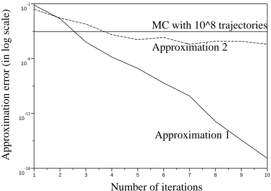
_{=I−P (which is an invertible matrix). At each iteration, we used} M=100 simulations per state. Figure 1 shows the L_∞approximation error (maxj∈XJ|V(j)−Vn(j)|)

in logarithmic scale, as a function of the iteration number 1≤n≤10. This approximation error (which is the true quantity of interest) is directly related to the variance of the estimates Vn.

For the approximation

A

_{1, we observe the geometric convergence to 0, as predicted in Theorem}

2. It takes less than 10×100 simulations per state to reach an error of 10−15. Using

A

_{2, the error}

does not decrease below some threshold'2.10−5 due to the approximation error V−

A

_{2V . This}

threshold is reached using about 5×100 simulations per state. For comparison, usual MC reaches an error of 10−4with 108simulations per state.

1 2 3 4 5 6 7 8 9 10 -16

10 -11 10

-6 10

-1 10

Approximation error (in log scale)

Number of iterations

MC with 10^8 trajectories

Approximation 2

Approximation 1

Figure 1: Approximation error for regular MC and sequential control variate algorithm using two approximations

A

_1and

A

_{2, as a function of the number of iterations.}

3. Gradient Estimation

Here, we assume that the transition matrix P depends on some parameterα, and that we wish to estimate the sensitivity of V(x) =E[Ψ(r,X(x))]with respect toα, which we write Z(x):=∂_αV(x).

An example of interest consists in solving approximately a Markov Decision Problem by search-ing for a feedback control law in a given class of parameterized stochastic policies. The optimal control problem is replaced by a parametric optimization problem, which may be solved (at least in order to find a local optimum) using gradient methods. Thus we are interested in estimating the gra-dient of the performance measure w.r.t. the parameter of the policy. In this example, the transition matrix P would be the transition matrix of the MDP combined with the parameterized stochastic policy.

As mentioned in the introduction, the gradient may be expressed as an expectation Z(x) = E[Φ(r,X(x))](using the so-called likelihood ratio or score method (Reiman and Weiss, 1986; Glynn, 1987; Williams, 1992; Baxter and Bartlett, 2001; Marbach and Tsitsiklis, 2003)) whereΦ(r,X(x))

is also a functional that depends on the trajectory X(x), and that is linear in its first variable. For example, in the discounted case (3), the functionalΦis given by (5). The variance is usually high, thus variance reduction techniques are highly needed (Greensmith et al., 2005).

The gradient Z is also the solution to the linear system (4). Unfortunately, this linear expression is not of the form (2) since∂_α

L

_{is not invertible, which prevents us from using directly the method}

of the previous section.

However, the linear equation (4) provides us with another representation for Z in terms of a probabilistic representation:

We may extend the previous algorithm to the estimation of Z by using two representations: Vn

and Zn. The approximation Vnof V is updated from Monte-Carlo estimation of the residual r−

L

Vn,

and Zn, which approximates Z, is updated from the gradient residual −∂α

L

Vn−

L

Zn built from

the current Vn. This approach may be related to the so-called Actor-Critic algorithms (Konda and

Borkar, 1999; Sutton et al., 2000), which use the representation (13) with an approximation of the value function.

A geometric variance reduction is also achieved, up to a threshold that depends on the approxi-mation errors of both of those representations.

Finally, we present a variance reduction technique that only makes use of the gradient repre-sentation Zn (which may be useful for Partially Observable MDPs) but at the cost of a variance

increase.

3.1 The Algorithm

Although the approximation operators for V and Z may be different in practice (they may use dif-ferent sets of representative states and basis functions), in this section, we will use the same approx-imation operator

A

_{for simplicity.}

From (13) and the equivalence property (8), we obtain the following representation for Z:

Z(x) =

A

_{Zn(x) +E}Ψ₍₋∂_α

L

_V−

L A

_Zn,X(x))

=

A

_{Zn(x) +E}Ψ₍₋∂_α

L

_(V−

A

_Vn),X(x))−Ψ₍∂_α

L A

_Vn+

L A

_Zn,X(x))

=

A

_{Zn(x) +E}Φ_(r−

L A

_Vn,X(x))−Ψ₍∂_α

L A

_Vn+

L A

_{Zn,X(x)). (14)}

from which the algorithm is deduced. We consider successive approximations Vn∈IRJ of V and

Zn∈IRJof Z defined at the states

X

J= (xj)1≤j≤J. • We initialize V0(xj) =0, Z0(xj) =0.

• At stage n, we simulate by Monte Carlo M trajectories(Xn,m(xj))1≤m≤M and define the new

approximations Vn+1and Zn+1at the states

X

J:

Vn+1(xj) =

A

Vn(xj) + 1

M

M

∑

m=1

Ψ(r−

L A

_Vn,Xn,m_(x j))

Zn+1(xj) =

A

Zn(xj) +

1

M

M

∑

m=1

h

Φ(r−

L A

_Vn,Xn,m_(xj))

−Ψ(∂_α

L A

_Vn+

L A

_Zn,Xn,m_(x j))

i .

3.2 Properties of the Estimates Vnand Zn

Expectation of Vnand Zn. We have already seen thatE[Vn] =V for all n>0. Now, (14) implies

thatEn[Zn+1] =Z, thusE[Zn] =Z for all n>0.

Variance of Vnand Zn. We write vn=sup1≤j≤JVar Vn(xj)and zn=sup1≤j≤JVar Zn(xj). The next

theorem (proved in Appendix B) states the geometric variance reduction for large enough values of

Theorem 4 We have

vn+1 ≤ ρMvn+

2

M

V

Ψ(V−

A

V)

zn+1 ≤ ρMzn+

2

M[c1(V−

A

V,Z−

A

Z) +c2vn] withρM=_M2 ∑Jj=1

p

V

_Ψ(φ_j)2_{, and the coefficients}

c1(f,g) =

q

V

_{Φ(f) +}

q

V

_Ψ(

L

−1∂_α

L

_{f) +}

q

V

_Ψ(g)2 c2 =

h J

∑

j=1

q

V

_Φ(φ_{j) +}q

V

_Ψ(

L

−1∂_α

L

φ_j)i2_,

using the notations

V

_Ψ(f):=sup

1≤j≤JVarΨ(

L

f,X(xj))and

V

Φ(f):=sup1≤j≤JVarΦ(

L

f,X(xj)).

Thus, for large enough values of M, (i.e. wheneverρM<1), the convergence of(vn)n and(zn)nis

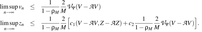
geometric at rateρM, up to the thresholds

lim sup

n→∞

vn ≤

1 1−ρM

2

M

V

Ψ(V−

A

V)

lim sup

n→∞

zn ≤

1 1−ρM

2

M

h

c1(V−

A

V,Z−

A

Z) +c2

1 1−ρM

2

M

V

Ψ(V−

A

V)

i .

Here also, if V and Z are representable by

A

_{, then the variance converges geometrically to 0.}

3.3 Numerical Experiment

Again we consider the Gambler’s ruin problem described previously. The transition matrix is pa-rameterized byα=p, the probability of winning. The gradient Z(i) =∂αV(i)may be derived from (12):

Z(i) = L(1−λ

i_)λL−1_−i(1−λL_)λi−1

(1−λL₎2α2 for i∈

X

,

(forα6=0.5), and Z(i) =0 forα=0.5. Again we use the representative states XJ ={1,7,13,19}.

Here, we consider two possible approximators

A

_1and

A

_{2for the value function representations Vn}

(as defined previously), and two approximators

A

_2and

A

_{3for the gradient representations Zn, where}

A

_{3 is the projection that uses K=3 functions}ψ_{1(i) =1,}ψ_{2(i) =}λi_,ψ

3(i) =iλi,i∈

X

. Notice that

Z is representable by

A

_{3but not by}

A

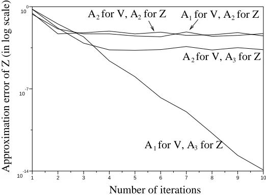
_{2. We choose p=0.51 and M=1000.}

Figure 2 shows the L∞approximation error of Z (maxj∈XJ|Z(j)−Zn(j)|) in logarithmic scale,

for the different possible approximations of V and Z.

When both V and Z may be perfectly approximated (i.e.

A

_{1 for V and}

A

_{3 for Z) we observe}

The variance reduction of this sequential method compared to regular MC is thus also consider-able.

1 2 3 4 5 6 7 8 9 10

-14 10

-7 10

0 10

Number of iterations

A for V, A for Z

A for V, A for Z2 1

2

Approximation error of Z (in log scale)

3 2

A for V, A for Z2

A for V, A for Z1 3

Figure 2: Approximation error of the gradient Z =∂_αV using approximators

A

_{1 and}

A

_{2 for the}

value function, and

A

_2and

A

_{3for the gradient.}

3.4 Variance Reduction with Only Z Representation

It would be desirable to design a similar variance reduction method using the gradient approximation only. However, as seen previously, the linear system (4) does not enable to recover r from the gradient (since∂_α

L

_{is not invertible), which prevents us from directly using the method of Section}

2.

Nevertheless, from (13), we have the representation for Z:

Z(x) =

A

_{Zn(x) +E}Φ_(r,X(x))−Ψ₍

L A

_Zn,X(x)),

from which we deduce the following algorithm: at stage n, simulate M trajectories Xn,mper state

(xj)and update the approximation Znaccording to

Zn+1(xj) =

A

Zn(xj) +

1

M

M

∑

m=1

h

Φ(r,Xn,m(xj))−Ψ(

L A

Zn,Xn,m(xj))

i .

Unfortunately, we may not expect this algorithm to exhibit a variance reduction to 0 in the case of perfect approximation of the gradient (i.e.

A

_{Z=Z). Indeed, there is an incompressible variance}

term that comes from the estimation ofΦ(r,X(x))instead ofΨ(

L

_{Z,X(x)) =}Ψ₍₋∂_α

L L

−1_r,X(x)).

To illustrate, in the infinite-horizon, discounted case (5), this incompressible variance term ap-pears in the estimation of

Φ(r,X(x))−Ψ(

L

_{Z,X(x)) =}

∑

t≥0

γth∂αP(xt,xt+1)

P(xt,xt+1) _s≥0

∑

γs+1_r(x

s+t+1)−(I−γP)Z(xt)

However this variance (which can be related to the variance of the value function V(xt+1)

esti-mation by the sum of future rewards∑_s≥0γsr(xs+t+1)and a bound on the likelihood ratios∂α_PP_(x(_tx_,t_x,_tx₊t+₁₎1))

is much lower (especially whenγis close to 1) than the initial variance of the direct estimation of

E[Φ(r,X(x))].

Thus, this algorithm would provide a geometric variance reduction, up to a threshold that de-pends on

V

_Ψ(Z−

A

_{Z) plus this incompressible variance term (the proof is a simple extension of}

that of Theorem 2 taking into account the additional variance term). This algorithm may be interest-ing in Partially Observable MDPs, and provide an alternative technique compared to other variance reduction techniques developed in this setting (Greensmith et al., 2005).

4. Conclusion

We described a sequential control variates method for estimating the expectation of functionals in Markov chains, using linear approximation (in the values). We illustrate the method on value function and gradient estimates. We proved geometric variance reduction up to a threshold that depends on the approximation error of the functions of interest.

There are several possible directions for future research, among which:

• Estimate the number of sample trajectories M per state that enables the method to exhibit a geometric variance reduction (i.e. wheneverρM<1).

• For a total budget of N trajectories per state, define what is the best trade-off between the number of iterations n and the number of trajectories M per iteration (such that N=nM).

• Define a stopping criterion (i.e. whenever there is no more variance decrease) from which we should continue (if needed) with a regular Monte Carlo method.

• Consider the case where the initial states are drawn according to some distribution over

X

instead of using the set of representative states

X

_J.

• Consider non-linear function approximation.

• Extend this work to a model-free, on-line learning framework.

Appendix A. Proof of Theorem 2

From the decomposition

V−

A

_Vn=V−

A

_V+

J

∑

i=1

(V−Vn)(xi)φi, (15)

we have

Vn+1(xj) =

A

Vn(xj) +

1

M

M

∑

m=1

h

Ψ(

L

_(V−

A

_V),Xn,m_(xj))

+ J

∑

i=1

(V−Vn)(xi)Ψ(

L

φi,Xn,m(xj))

Thus

VarnVn+1(xj) =

1

MVar

n_Ψ(

_L

_(V−

_A

_V),X(x j))

+ J

∑

i=1

(V−Vn)(xi)Ψ(

L

φi,X(xj))

.

We use the general bound

Var

∑

i

αiYi

=

∑

i1,i2

αi1αi2Cov(Yi1,Yi2)

≤

∑

i1,i2

|αi1||αi2| q

Var[Yi1] q

Var[Yi2]≤

∑

i |αi|

p

Var[Yi]

2

, (16)

for any real numbers(αi)iand square integrable real random variables(Yi)i, to deduce that

VarnVn+1(xj) ≤

1

M

hq

V

_Ψ(V−

A

_{V) +}

J

∑

i=1

|V−Vn|(xi)

q

V

_Ψ(φ_i)i2_{, (17)}

with

V

_Ψ(f):=sup

1≤j≤JVarΨ(

L

f,X(xj)).Now, we use the variance decomposition

Var Vn+1(xj) = Var[En[Vn+1(xj)]] +E[Varn[Vn+1(xj)]]

= E[Varn[Vn+1(xj)]],

and the general bound (deduced similarly to (16))

E(α0+ J

∑

i=1

αiYi)2

≤2α2₀+2

J

∑

i=1 |αi|

q

E[Y_i2]2, (18) to deduce from (17) that

vn+1 ≤

2

M

_V

Ψ(V−

A

_{V) +}

J

∑

i=1

q

V

_Ψ(φ_i)2_vn,

which gives (10). Now, if M is such thatρM:=_M2 ∑Ji=1

p

V

_Ψ(φ_i)2_{<1, then taking the upper limit}

finishes the proof of Theorem 2.

Appendix B. Proof of Theorem 4

Using (4) and (6), we have the decomposition

−∂α

L A

Vn−

L A

Zn = −∂α

L A

(Vn−V)−∂α

L

(

A

V−V)

+

L

_(Z−

A

_{Z) +}

L A

_(Z−Zn)

= J

∑

i=1

(V−Vn)(xi)∂α

L

φi−∂α

L

(

A

V−V)

+

L

_(Z−

A

_{Z) +}

J

∑

i=1

Now, using (15), the variance may be written

VarnZn+1(xj) =

1

MVar

nh_Φ(

_L

_(V−

_A

_V),X(x j))

+ J

∑

i=1

(V−Vn)(xi)Φ(

L

φi,X(xj))−Ψ(∂α

L

(

A

V−V),X(xj))

+ J

∑

i=1

(V−Vn)(xi)Ψ(∂α

L

φi,X(xj)) +Ψ(

L

(Z−

A

Z),X(xj))

+ J

∑

i=1

(Z−Zn)(xi)Ψ(

L

φ_i,X(xj))i_.

We use (16) to deduce the bound

VarnZn+1(xj) ≤

1

M

hq

V

_Φ(V−

A

_{V) +}

q

V

_Ψ(

L

−1∂_α

L

₍

A

_V−V))

+ J

∑

i=1

|V−Vn|(xi)

q

V

_Φ(φ_{i) +}

q

V

_Ψ(

L

−1∂_α

L

φ_i)

+

q

V

_Ψ(Z−

A

_{Z) +}

J

∑

i=1

|Z−Zn|(xi)

q

V

_Ψ(φ_i)i2_,

Now, we use (18) to deduce that

zn+1 ≤

2

M

n q

V

_Φ(V−

A

_{V) +}

q

V

_Ψ(

L

−1∂_α

L

₍

A

_V−V))

+h

J

∑

i=1

q

V

_Φ(φ_{i) +}

q

V

_Ψ(

L

−1∂_α

L

φ_i)i2_vn

+

q

V

_Ψ(Z−

A

_{Z) +}h

J

∑

i=1

q

V

_Ψ(φ_i)i2_zno_,

and Theorem 4 follows.

References

C. G. Atkeson, S. A. Schaal, and Andrew W. Moore. Locally weighted learning. AI Review, 11, 1997.

J. Baxter and P. L. Bartlett. Infinite-horizon gradient-based policy search. Journal of Artificial

Intelligence Research, 15:319–350, 2001.

P. W. Glynn. Likelihood ratio gradient estimation: an overview. In A. Thesen, H. Grant, and W. D. Kelton, editors, Proceedings of the 1987 Winter Simulation Conference, pages 366–375, 1987.

E. Gobet and S. Maire. Sequential control variates for functionals of Markov processes. SIAM

E. Greensmith, P. L. Bartlett, and J. Baxter. Variance reduction techniques for gradient estimates in reinforcement learning. Journal of Machine Learning Research, 5:1471–1530, 2005.

J. H. Halton. A retrospective and prospective survey of the Monte-Carlo method. SIAM Review, 12 (1):1–63, 1970.

J. H. Halton. Sequential Monte-Carlo techniques for the solution of linear systems. Journal of

Scientific Computing, 9:213–257, 1994.

J. M. Hammersley and D. C. Handscomb. Monte-Carlo Methods. Chapman and Hall, 1964.

T. Hastie, R. Tibshirani, and J. Friedman. The Elements of Statistical Learning. Springer Series in Statistics, 2001.

C. Kollman, K. Baggerly, D. Cox, and R. Picard. Adaptive importance sampling on discrete Markov chains. The Annals of Applied Probability, 9(2):391–412, 1999.

V. R. Konda and V. S. Borkar. Actor-critic-type learning algorithms for Markov decision processes.

SIAM Journal of Control and Optimization, 38:1:94–123, 1999.

S. Maire. An iterative computation of approximations on Korobov-like spaces. J. Comput. Appl.

Math., 54(6):261–281, 2003.

P. Marbach and J. N. Tsitsiklis. Approximate gradient methods in policy-space optimization of Markov reward processes. Journal of Discrete Event Dynamical Systems, 13:111–148, 2003.

M. I. Reiman and A. Weiss. Sensitivity analysis via likelihood ratios. In J. Wilson, J. Henriksen, and S. Roberts, editors, Proceedings of the 1986 Winter Simulation Conference, pages 285–289, 1986.

R. S. Sutton, D. McAllester, S. Singh, and Y. Mansour. Policy gradient methods for reinforcement learning with function approximation. Neural Information Processing Systems. MIT Press, pages 1057–1063, 2000.

V. Vapnik. Statistical Learning Theory. John Wiley & Sons, New York, 1998.

V. Vapnik, S. E. Golowich, and A. Smola. Support vector method for function approximation, regression estimation and signal processing. In Advances in Neural Information Processing

Sys-tems, pages 281–287, 1997.