Dynamic Weighted Majority: An Ensemble Method
for Drifting Concepts
∗J. Zico Kolter [email protected]
Department of Computer Science Stanford University
Stanford, CA 94305-9025, USA
Marcus A. Maloof† [email protected] Department of Computer Science
Georgetown University
Washington, DC 20057-1232, USA
Editor: Dale Schuurmans
Abstract
We present an ensemble method for concept drift that dynamically creates and removes weighted experts in response to changes in performance. The method, dynamic weighted majority (DWM), uses four mechanisms to cope with concept drift: It trains online learners of the ensemble, it weights those learners based on their performance, it removes them, also based on their performance, and it adds new experts based on the global performance of the ensemble. After an extensive evaluation— consisting of five experiments, eight learners, and thirty data sets that varied in type of target con-cept, size, presence of noise, and the like—we concluded thatDWMoutperformed other learners that only incrementally learn concept descriptions, that maintain and use previously encountered examples, and that employ an unweighted, fixed-size ensemble of experts.
Keywords: concept learning, online learning, ensemble methods, concept drift
1. Introduction
In this paper, we describe an ensemble method designed expressly for tracking concept drift (Kolter and Maloof, 2003). Ours is an extension of the weighted majority algorithm (Littlestone and War-muth, 1994), which also tracks drifting concepts (Blum, 1997), but our algorithm, dynamic weighted majority (DWM), adds and removes base learners or experts in response to global and local perfor-mance. As a result,DWMis better able to respond in non-stationary environments.
Informally, concept drift occurs when a set of examples has legitimate class labels at one time and has different legitimate labels at another time. Naturally, over some time scale, the set of examples and the change they undergo must produce a measurable effect on a learner’s performance. Concept drift is present in many applications, such as intrusion detection (Lane and Brodley, 1998)
∗. Based on “Dynamic Weighted Majority: A new ensemble method for tracking concept drift”, by Jeremy Z. Kolter and Marcus A. Maloof, which appeared in the Proceedings of the Third IEEE International Conference on Data Mining.
c
and credit card fraud detection (Wang et al., 2003). Indeed, tracking concept drift is important for any application involving models of human behavior.
In previous work, we evaluated DWM using two synthetic data sets, the STAGGER concepts (Schlimmer and Granger, 1986) and the SEAconcepts (Street and Kim, 2001), achieving the best published results (Kolter and Maloof, 2003). Using the STAGGER concepts, we also made a di-rect comparison to Blum’s (1997) implementation of weighted majority (Littlestone and Warmuth, 1994).
Here, we present additional results for theSTAGGERdata set by making a direct comparison to our implementation of theSTAGGERlearning system (Schlimmer and Granger, 1986) and to a series of rule learners for concept drift that use theAQalgorithm: AQ-PM(Maloof and Michalski, 2000), AQ11-PM (Maloof and Michalski, 2004), and AQ11-PM+WAH (Maloof, 2003). We also present results for two real-world data sets. The first is the CAP data set (Mitchell et al., 1994), which Blum (1997) used to evaluate his implementation of weighted majority. The second is a data set for electricity pricing, which Harries (1999) used to evaluate Splice2. Finally, we include results for twenty-sixUCI data sets (Asuncion and Newman, 2007) because we were interested in evaluating DWM’s performance on static concepts.
Overall, results suggest that a weighted ensemble of incremental learners tracks drifting con-cepts better than learners that simply modify concept descriptions, that store and learn from exam-ples encountered previously, and that use an unweighted ensemble of experts. AlthoughDWMhas no advantage over a single base learner for static concepts, results from 26UCIdata sets show that, overall,DWMperforms no worse than a single base learner.
We cite two main contributions of this work. First, we present a general algorithm for using any online learning algorithm for problems with concept drift. Second, we present results of an extensive empirical study characterizing DWM’s performance along several dimensions: with different base learners, with well-studied data sets, with class noise, with static concepts, and with respect to learners appearing previously in the literature.
The organization of the paper is as follows. In the next section, we survey work on the problem of concept drift, on ensemble methods, and at the intersection: work on ensemble methods for con-cept drift. In Section 3, we describe dynamic weighted majority, an ensemble method for tracking concept drift. In Section 4, we present the results of our empirical study. Section 5 concludes the paper, and it is here that we discuss directions for future research.
2. Background and Related Work
Dynamic weighted majority is an ensemble method designed expressly for concept drift. For many years, research on ensemble methods and research on methods for concept drift have intermingled little. However, within the last few years, researchers have proposed several ensemble methods for tracking concept drift. In the next three sections, we survey relevant work on the problem of tracking concept drift, on ensemble methods, and on ensemble methods for tracking concept drift.
2.1 Concept Drift
they can change their shape, size, and location. In concrete terms, concept drift occurs when the class labels of a set of examples change over time. Researchers have used both real (e.g., Harries and Horn, 1995; Blum, 1997; Lane and Brodley, 1998; Harries, 1999; Black and Hickey, 2002; Gramacy et al., 2003; Wang et al., 2003; Gama et al., 2004; Delany et al., 2005; Gama et al., 2005; Scholz and Klinkenberg, 2005; Tsymbal et al., 2005) and synthetic (e.g., Schlimmer and Granger, 1986; Widmer and Kubat, 1996; Maloof and Michalski, 2000; Hulten et al., 2001; Street and Kim, 2001; Kolter and Maloof, 2003; Klinkenberg, 2004; Maloof and Michalski, 2004; Gama et al., 2005; Kolter and Maloof, 2005; Scholz and Klinkenberg, 2005) data sets as inspiration for and the evaluation of a variety of methods for tracking concept drift. There has also been theoretical work on this problem (e.g., Helmbold and Long, 1991; Kuh et al., 1991; Helmbold and Long, 1994; Auer and Warmuth, 1998; Mesterharm, 2003; Monteleoni and Jaakkola, 2004; Kolter and Maloof, 2005), but a thorough survey of this work is beyond the scope of the paper.
STAGGER (Schlimmer and Granger, 1986) was the first system designed to cope with concept drift. It uses a distributed concept description consisting of class nodes linked to attribute-value nodes by probabilistic arcs. Two probabilities associated with each arc represent necessity and sufficiency, and are updated based on a psychological theory of association learning (Rescorla, 1968). In addition to adjusting these probabilities when new training examples arrive, STAGGER can also add nodes corresponding to new classes and new features. To better cope with concept drift, STAGGER may decay its probabilities over time. Empirical results on a synthetic data set, now known as theSTAGGERconcepts, show the method acquiring three changing target concepts in succession. TheSTAGGERconcepts have been a centerpiece of numerous evaluations (Widmer and Kubat, 1996; Widmer, 1997; Maloof and Michalski, 2000; Kolter and Maloof, 2003; Maloof and Michalski, 2004; Kolter and Maloof, 2005), and we discuss them further in Section 4.1.
Concept versioning (Klenner and Hahn, 1994) is a method for coping with gradual or evolu-tionary concept drift. It uses a frame representation and copes with such drift by either adjusting
current concept descriptions or creating a new version of these descriptions. The system creates a new version when an instance’s attribute values and ranges present in current concept descriptions are dissimilar, based on a measure that accounts for both quantitative (e.g., value differences) and qualitative (e.g., increasing trend) information. Empirical results, based on 124 examples of com-puters sold between 1987 and 1993, suggest that the system acquired three versions of concepts based on machines’ clock frequency and memory size.
TheFLORAsystems (Widmer and Kubat, 1996) track concept drift by maintaining a sequence of examples over a dynamically adjusted window of time and using them to induce and refine three sets of rules: rules covering the positive examples, rules covering the negative examples, and potential rules that are, at present, too general. Examples entering and leaving the window causeFLORAto refine rules, to move them from one set to another, or to delete them. FLORA2 uses just these basic mechanisms, whereas FLORA3 is an extension that handles recurring contexts. FLORA4 extends FLORA3 with mechanisms for coping with noise, similar to those present inIB3 (Aha et al., 1991). On theSTAGGER concepts, the method generally performed well in terms of slope and asymptote after concepts changed. (We further analyze these results in Section 4.1.)
relevant concept of warm. As an agent moves from one season to the next, it uses the contextual variable to better focus the base algorithm on those features relevant for learning and prediction.
Meta-learning mechanisms identify contextual attributes by maintaining co-occurrence and fre-quency counts over the learner’s entire history and over a fixed window of time. Using a χ2 test, the meta-learning algorithm identifies contextual features and those predictive features relevant for the given context. The base learner then uses the predictive features of the contextually relevant examples in the current window to form new concept descriptions. By adding a contextual variable to the STAGGER concepts (Schlimmer and Granger, 1986), experimental results using predictive accuracy suggest that the meta-learners were able use contextual features to acquire target concepts better than and more quickly than did the base learners alone. When compared toFLORA4 (Widmer and Kubat, 1996), which retrieves previously learned concept descriptions when contexts reoccur, MetaL(B) often performed better in terms of slope and asymptote, even though it relearned new concept descriptions rather than retrieving and modifying old ones.
Lane and Brodley (1998) investigated methods for concept drift in one-class learning problems (i.e., anomaly detection). For an intrusion detection domain, they used instance-based learning in which instances were fixed-length sequences ofUNIXcommands. As a user enters new commands, the system calculates a measure of similarity between the current instance and past instances. They investigated two methods for coping with concept drift. One fits a line to the sequence of similarity measures in a window and uses its direction and magnitude to adjust the decision threshold. A second uses the slope of the line to determine if there is a stable or changing trend and inserts new examples into a user profile only if the trend is changing. Both methods proved useful in striking the delicate balance between learning a user’s changing behavior and detecting anomalous behavior.
CD3 (Black and Hickey, 1999) usesID3 (Quinlan, 1986) to learn online from batches of training data. The method maintains a collection of examples from the stream, all annotated with a time stamp of current. It annotates examples in a new training batch with a stamp of new. For static concepts, the time stamp is an irrelevant attribute, but if drift occurs, then the time stamp will appear in induced trees. Moreover, one can use its position in the tree as an indicator of how much drift may have occurred—the more relevant the time stamp, the higher it will appear in the tree, and the more drift that has occurred. After pruning, the method produces a set of valid and invalid rules by enumerating paths in the tree with new and current time stamps, respectively. Rule conditions containing a time stamp are then removed.
The performance element uses the valid rules for prediction, and the method uses the invalid rules to remove outdated examples from its store. However, depending on parameter settings, if both an invalid and a valid rule cover a stored example, then the method removes the example. Results from an empirical study involving synthetic data and varying amounts of class noise suggest thatCD3 copes with revolutionary and evolutionary concept drift better than—in terms of slope and asymptote—ID3 learning from only the most recent batch and better than ID3 learning from all previously encountered batches.
CD4 (Hickey and Black, 2000) extends CD3 by letting time stamps for a batch be numeric, although the method no longer uses invalid rules to remove stored examples. CD5 (Hickey and Black, 2000) extendsCD4 by assigning numeric time stamps to individual examples, rather than to batches. In an empirical study with synthetic data and evolutionary and revolutionary changes in target concepts, all three systems performed comparably.
induced decision trees. Indeed, during one period, the time stamp was the most relevant attribute and at the root of the decision tree.
Syed et al. (1999) present an online algorithm for training support vector machines (Boser et al., 1992). The method adds previously obtained support vectors to the new training set and then builds another machine. When compared to a batch algorithm, the online method performed comparable on severalUCIdata sets (Asuncion and Newman, 2007). The authors pointed to drops and recoveries in predictive accuracy during the incremental runs as evidence thatSVMs can handle drift.
The presence of drops and recoveries are necessary for detecting concept drift, but they are not sufficient. The drops in predictive accuracy could have been due to sampling, and in general, it may be difficult to determine if a learner is coping with concept drift or is simply acquiring more information about a static concept. This type of concept drift has been called virtual concept drift, as opposed to real concept drift (Klinkenberg and Joachims, 2000). Indeed, the data sets included in the evaluation (e.g.,monks,sonar, andmushroom) are not typically regarded as having concepts that drift.
Kelly et al. (1999) define population drift as being “related to” concept drift, noting that the term concept drift has no single meaning. They define population drift as change in the problem’s probability distribution. Such changes can occur in the prior, conditional, and posterior distribu-tions, and using artificial data, they analyze the impact on performance of changes to each of these distributions.
The term concept drift has been applied to different phenomena, such as drops and recoveries in performance during online learning (Syed et al., 1999). However, in concrete terms, the term has historically meant that the class labels of instances change over time, established in the first paper on concept drift (Schlimmer and Granger, 1986). Such change corresponds to change in the posterior distribution and in the conditional distribution. However, the prior distribution may not change, and changes in the conditional distribution will not necessarily mean that concept drift has occurred.
Klinkenberg and Joachims (2000) used a support vector machine to size windows for concept drift. Rather than tuning parameters for an adaptive windowing heuristic (c.f. Widmer and Kubat, 1996), the algorithm sizes the window by minimizing generalization error on new examples. Upon receiving a new batch of examples, the method generates support vector machines with various sizes of windows using previously encountered batches of training examples, and selects the window size that minimizes theξα-estimate, an approximation to the leave-one-out or jackknife estimator (Hinkley, 1983). Experimental results on a manually constructed data set derived from 2,608 news documents suggest that exhaustively searching for a window’s size was better, in terms of slope and asymptote of predictive accuracy, than a window of fixed size. Results from subsequent experiments indicate that selecting examples in batches or using an adaptive window yielded higher precision and recall than did weighting examples based on their age or their fit to the current model (Klinkenberg, 2004).
and Larson, 1983) andGEM(Reinke and Michalski, 1988) algorithms, respectively, to form rules. Finally,AQ11-PM+WAHis an extension ofAQ11-PMthat uses Widmer and Kubat’s (1996) window adjustment heuristic (WAH) to dynamically size the window of time over which examples are kept. TheSTAGGERconcepts were the centerpiece in the evaluation of all of these systems.
The Concept-adapting Very Fast Decision Tree (CVFDT) learner (Hulten et al., 2001) extends VFDT(Domingos and Hulten, 2000) by adding mechanisms for handling concept drift.VFDTgrows a decision tree only from its leaf nodes, so there is no restructuring of the tree (cf. sc iti, Utgoff et al., 1997). The method maintains a decision tree and maintains counts of attribute values for classes in each leaf node. New examples propagate through the tree to a leaf node with the algorithm updating the counts. If the propagated examples and the examples used to form a leaf node are not of the same class, then the method uses a splitting criterion and the Hoeffding (1963) bound to determine if the node should be split.
CVFDT extendsVFDT by maintaining at each node in the tree a list of alternate subtrees and attribute-value counts for each class. LikeVFDT, new examples propagate through the tree to a leaf node, but they also propagate through all of the alternate subtrees along this path. Periodically, the method forgets examples, and if an alternate subtree is more accurate than the current one, it swaps them. Empirical results on a synthetic data set consisting of a rotating hyperplane, five million training examples, and drift every 50,000 time steps, suggest thatCVFDTproduced smaller, more accurate trees than didVFDT.
2.2 Ensemble Methods
Ensemble methods maintain a collection of learners and combine their decisions to make an overall
decision. Generally, an algorithm applied multiple times to the same data set will produce identical classifiers that make the same decisions, so for ensemble methods to work, there must be some mechanism to produce different classifiers. This is accomplished by either altering the training data or the learners in the collection.
Bagging (Breiman, 1996) is one of the simplest ensemble methods. It entails producing a set of bootstrapped data sets from the original training data. This involves sampling with replacement from the training data and producing multiple data sets of the same size. Once formed, a learning method produces a classifier from each bootstrapped data set. During performance, the method predicts based on a majority vote of the predictions of the individual classifiers.
Weighted majority (Littlestone and Warmuth, 1994), instead of using altered training sets, relies on a collection of different classifiers, often referred to as “experts.” Each expert begins with a weight of one, which is decreased (e.g., halved) whenever an expert predicts incorrectly. To make an overall prediction, the method takes a weighted vote of the expert predictions, and predicts the class with the most weight. Winnow is a similar algorithm, but also increases the weights of experts that predict correctly (Littlestone, 1991).
Stacked generalization or stacking (Wolpert, 1992), like weighted majority, is an ensemble method for combining the decisions of different types of learners. However, stacking uses the predictions of the base learners to form training examples for a meta-learner. Stacking begins by partitioning the original examples into three sets: training, validation, and testing. The method trains the base learners using the training data and then applies the resulting classifiers to the ex-amples in the validation set. Using the predictions of the exex-amples as features and their original class labels, it forms a new training set, which it uses to train the meta-learner. After training the meta-learner with these examples, performance entails presenting an instance to the base classifiers, using their predictions as input to the meta-classifier. The method’s overall prediction is that of the meta-classifier.
There have been numerous studies of ensemble methods (e.g., Hansen and Salamon, 1990; Woods et al., 1997; Quinlan, 1996; Zheng, 1998; Opitz and Maclin, 1999; Bauer and Kohavi, 1999; Maclin and Opitz, 1997; Dietterich, 2000; Zhou et al., 2002; Chawla et al., 2004), and we cannot survey them all. Generally, this research suggests that ensemble methods outperform single classi-fiers on many standard data sets (Opitz and Maclin, 1999). Boosting is generally better than bagging (Bauer and Kohavi, 1999; Opitz and Maclin, 1999; Dietterich, 2000), although bagging seems more robust to noise than is boosting (Dietterich, 2000). Analysis suggests that ensemble methods work by reducing bias, variance, or both (Breiman, 1998; Bauer and Kohavi, 1999; Zhou et al., 2002).
Popular ensemble methods, such as bagging and boosting, are off-line algorithms, but re-searchers have developed online ensemble methods. Winnow (Littlestone, 1988) and weighted majority (Littlestone and Warmuth, 1994) fall into this category, as do Blum’s (1997) versions of these algorithms.
Online AdaBoost (Fan et al., 1999), when a new batch of examples arrives, weights the examples and then re-weights the ensemble’s classifiers based on their performance on the new examples. The method then builds a new classifier from the new, weighted examples. For efficiency, the method retains only the k most recent classifiers.
Online arcing (Fern and Givan, 2003) uses incremental base learners and incrementally updates their voting weights. When a new training instance arrives, for each classifier in the ensemble, the method first increases the classifier’s voting weight by one if the classifier correctly classifies the new instance. The method then computes an instance weight for the classifier based on the number of other classifiers in the ensemble that misclassify the instance. Finally, an incremental learning function uses the instance and the weight to refine the classifier. The method may use a weighted or unweighted voting scheme to classify an instance.
2.3 Ensemble Methods for Concept Drift
Ensemble methods for concept drift share many similarities with the online and off-line methods discussed in the previous section. However, methods for concept drift must take into account the temporal nature of the data stream, for a set of examples may have certain class labels at time t and others at time t0.
Any method for coping with changing concepts must have mechanisms for refining or removing knowledge of past target concepts. To achieve these effects, one ensemble method for concept drift builds two ensembles and selects the best performing one for subsequent processing (Scholz and Klinkenberg, 2006). Other methods replace poorly performing members of the ensemble (Street and Kim, 2001; Fan, 2004), decrease the effect these members have on the overall prediction (Blum, 1997; Scholz and Klinkenberg, 2006), or both (Kolter and Maloof, 2003; Wang et al., 2003; Kolter and Maloof, 2005).
Blum’s (1997) implementation of the weighted majority algorithm (Littlestone and Warmuth, 1994) uses as experts pairs of features coupled with a history of the most recent class labels from the training set appearing with those features. When a new instance arrives, the expert for a given pair of features predicts based on a majority vote of the labels of past observations. The global algorithm predicts based on a weighted-majority vote of the expert predictions and decreases the weight of any expert that predicts incorrectly. Each expert then stores the correct prediction in its history.
Blum (1997) also investigated triples of features as experts and a variant of winnow (Littlestone, 1988) that lets experts abstain if their features are not present in an instance. On a calendar schedul-ing task, which we describe further in Section 4.3, these methods were able to track a professor’s preferences for scheduling meetings across semester boundaries.
The Streaming Ensemble Algorithm (SEA) maintains a fixed-size collection of classifiers, each built from a batch of training examples (Street and Kim, 2001). When a new batch of examples arrives,SEAusesC4.5 (Quinlan, 1993) to build a decision tree. If there is space,SEAadds the new classifier to the ensemble. Otherwise, if the new classifier outperforms a classifier in the ensemble, SEA replaces it with the new one. Performance is measured on the current batch of examples. Overall,SEApredicts based on a majority vote of the predictions of the classifiers in the ensemble. An evaluation using a synthetic data set generated from shifting a hyperplane revealed that the method was able to acquire a series of four changing target concepts with accuracy of about 92%. We discuss this data set further in Section 4.2.
Herbster and Warmuth (1998) consider a setting in which an online learner is trained over sev-eral concepts and has access to n experts (which are fixed prediction strategies). They present an algorithm that performs almost as well as the best expert on each concept individually, paying an additional penalty of log n on each concept. Bousquet and Warmuth (2002) extend this setting to one where the best expert always comes from a smaller pool of mn experts. Here they show
that the learner can pay a log m rather than a log n penalty on each concept, plus a one-time cost of log mnto identify the best m experts.
The Accuracy-weighted Ensemble (AWE) also maintains a fixed-size collection of classifiers built from batches of training examples, but this method weights each classifier based on its perfor-mance on the most recent batch (Wang et al., 2003). If there is space in the ensemble, thenAWEadds the new weighted classifier. Otherwise, it keeps only the top k weighted classifiers. AWEpredicts based on a weighted-majority vote of the predictions of the ensemble’s classifiers. The evaluation of this method involved a synthetic data set generated from a rotating hyperplane and a data set for credit card fraud detection. Although the evaluation consisted of many experimental conditions, such as how the problem’s dimension affects error rate of the ensemble classifier, it did not include measuring the system’s performance over time and over changing target concepts.
to differences in their weighting schemes. DWMsets the weight of a new expert to one, whereas AddExp sets a new expert’s weight to the total weight of the ensemble times some parameterγ∈
(0,1). In addition to empirical results, the authors present worst-case bounds for the algorithm’s loss and number of mistakes, proving that AddExp performs almost as well as the best-performing expert. They also describe two pruning methods for limiting the number of experts maintained; one is useful in practice, the other gives formal guarantees on the number of experts that AddExp will create.
3. DWM: An Ensemble Method for Concept Drift
Dynamic weighted majority maintains a weighted pool of experts or base learners. It adds and removes experts based on the global algorithm’s performance. If the global algorithm makes a mistake, thenDWM adds an expert. If an expert makes a mistake, then DWMreduces its weight. If, in spite of multiple training episodes, an expert performs poorly, as indicated by a sufficiently low weight, thenDWMremoves it from the ensemble. This method is general, and in principle, one could use any online learning algorithm as a base learner. One could also use different types of base learners, although one would also have to implement control policies to determine what base learner to add.
The formal algorithm forDWMappears in Figure 1. The algorithm maintains a set of m experts,
E, each with a weight, wi for i=1, . . . ,m. Input to the algorithm is n training examples, each
consisting of a feature vector and a class label. The parameters also include the number of classes (c) and β, a multiplicative factor that DWM uses to decrease an expert’s weight when it predicts incorrectly. A typical value for β is 0.5. The parameter θ is a threshold for removing poorly performing experts. If an expert’s weight falls below this threshold, thenDWMremoves it from the ensemble. Finally, the parameter p determines how oftenDWMcreates and removes experts. We found this parameter useful and necessary for large or noisy problems, which we discuss further in Section 4.2. In the following discussion, we assume p=1.
DWMbegins by creating an ensemble containing a single learner with a weight of one (lines 1–3 of Figure 1). Initially, this learner could predict a default class, or it could predict using previous experience, background knowledge, or both. DWMthen takes a single example (or perhaps a set of examples) from the stream and presents it to the single learner to classify (line 7). If the learner’s prediction is wrong (line 8), thenDWMdecreases the learner’s weight by multiplying it byβ(line 9). Since there is one expert in the ensemble, its prediction isDWM’s global prediction (lines 12 and 24). IfDWM’s global prediction is incorrect (line 16), then it creates a new learner with a weight of one (lines 17–19).DWMthen trains the experts in the ensemble on the new example (line 23). After training,DWMoutputs its global prediction (line 24).
When there are multiple learners,DWMobtains a classification from each member of the ensem-ble (lines 6 and 7). If one’s prediction is incorrect, thenDWMdecreases its weight (lines 8 and 9). Regardless of the correctness of the prediction,DWMuses each learner’s prediction and its weight to compute a weighted sum for each class (line 10). The class with the most weight is set as the global prediction (line 12).
Dynamic-Weighted-Majority({~x,y}1n,c,β,θ,p)
{~x,y}1n: training data, feature vector and class label
c∈N∗: number of classes, c≥2
β: factor for decreasing weights, 0≤β<1 θ: threshold for deleting experts
p: period between expert removal, creation, and weight update {e,w}1m: set of experts and their weights
Λ,λ∈ {1, . . . ,c}: global and local predictions ~σ∈Rc: sum of weighted predictions for each class
1. m←1
2. em←Create-New-Expert() 3. wm←1
4. for i←1, . . . ,n // Loop over examples 5. ~σ←0
6. for j←1, . . . ,m // Loop over experts 7. λ←Classify(ej,~xi)
8. if(λ6=yiand i mod p=0)
9. wj←βwj
10. σλ←σλ+wj
11. end;
12. Λ←argmaxjσj
13. if(i mod p=0)
14. w←Normalize-Weights(w)
15. {e,w} ←Remove-Experts({e,w},θ)
16. if(Λ6=yi)
17. m←m+1
18. em←Create-New-Expert()
19. wm←1
20. end;
21. end;
22. for j←1, . . . ,m
23. ej←Train(ej,~xi,yi) 24. outputΛ
end; end.
last expert in the ensemble. As mentioned previously, if the global prediction is incorrect (line 16), DWM adds a new expert to the ensemble with a weight of one (lines 17–19). Finally, after using the new example to train each learner in the ensemble (lines 22 and 23), DWMoutputs the global prediction, which is the weighted vote of the expert predictions (line 24).
As mentioned previously, the parameter p letsDWMbetter cope with many or noisy examples.
p defines the period over whichDWMwill not update learners’ weights (line 8) and will not remove
or create experts (line 13). During this period, however,DWMstill trains the learners (lines 22 and 23).
DWM is a general algorithm for coping with concept drift. One can use any online learning algorithm as the base learner. To date, we have evaluated two such algorithms, naive Bayes and Incremental Tree Inducer, and we describe these versions in the next two sections.
3.1 DWM-NB
DWM-NBuses an incremental version of naive Bayes as the base learner. For this study, we used the implementation fromWEKA(Witten and Frank, 2005), which stores for nominal attributes a count for each class and for each attribute value given the class. The count is simply the number of times each class or attribute value appears in the training set, and so the learning element increments the appropriate counts when processing a new example. The performance element uses these counts to compute estimates of the prior probability of each class, P(Ci), and the conditional probability of each attribute value given the class, P(vj|Cj). It then operates under the assumption that attributes are conditionally independent and uses Bayes’ rule to predict the most probable class:
C=argmax Ci
P(Ci)
∏
j
P(vj|Ci).
For numeric attributes, it stores the sum of an attribute’s values and the sum of the squared values. Given a value, vj,
P(vj|Ci) =
1 σi j√2πe−
(vj−µi j)2/2σ2i j ,
where µi j is the average of the jth attribute’s values for the ith class, and σi j is their standard deviation. The performance element computes these values from the stored sums.
3.2 DWM-ITI
Like standard decision tree algorithms, given an observation, the performance element uses the observation’s attributes and their values to traverse from the root node to an external node. It predicts the class label stored in the node.
ITI updates a tree by propagating a new example to a leaf node. During the descent, the al-gorithm updates the information stored at each node—counts or values—and upon reaching a leaf node, determines if the tree should be extended by converting the leaf node to a decision node. A secondary process examines whether the tests at each node are most appropriate, and if not, restruc-tures the tree accordingly.
As one can imagine, for large problems, storing all examples at leaf nodes and restructuring decision trees can be costly, especially when maintaining an ensemble of such trees. While we were judicious when applyingDWM-ITI to large problems, as we see in the next section, where we discuss our experimental study, the learner performed well in spite of these potential costs.
4. Empirical Study and Results
In this section, we present experimental results for DWM-NB and DWM-ITI. We conducted five evaluations. The first, most extensive evaluation involved the STAGGERconcepts (Schlimmer and Granger, 1986), a standard benchmark for evaluating how learners cope with drifting concepts. In this evaluation, we compared the performance ofDWM-NBandDWM-ITI
1. to best- and worst-case base learners,
2. to our implementation ofSTAGGER(Schlimmer, 1987),
3. toAQ-PM(Maloof and Michalski, 2000),AQ11-PM(Maloof and Michalski, 2004), andAQ 11-PM+WAH(Maloof, 2003), and
4. to Blum’s (1997) implementation of weighted majority.
To the best of our knowledge, ours are the only results for Blum’s algorithm on the STAGGER concepts.
In an effort to determine how our method scales to larger problems involving concept drift, our second evaluation consisted of testing DWM-NB using the SEA concepts (Street and Kim, 2001), a problem recently proposed in the data mining community. For the third evaluation, we applied DWM-NBto theCAPdata set, a calendar scheduling task (Mitchell et al., 1994). Blum (1997) used this problem to evaluate weighted majority and winnow. For the fourth, we evaluatedDWM-NBon the task of predicting the price of electricity in New South Wales, Australia, between May 1997 and December 1999, a problem originally introduced by Harries (1999).
Finally, although it is clear that DWM should have no advantage over a single learner when acquiring static concepts, for the sake of completeness, we evaluatedDWM-NBon twenty-six data sets from theUCIRepository (Asuncion and Newman, 2007). The intent of this evaluation was to show that, on static concepts,DWMperforms no worse than a single base learner.
4.1 TheSTAGGERConcepts
S M L T C R C T R C R T Size Red Green Blue Shape Color
S M L T C R C T R C R T Size Red Green Blue Shape Color
S M L T C R C T R C R T Size Red Green Blue Shape Color
Target Target Target
concept concept concept
t=1. . .40. t=41. . .80. t=81. . .120.
Figure 2: Visualization of theSTAGGERConcepts (Maloof and Michalski, 2000). c2000 Kluwer Academic Publishers. Used with permission.
medium, large}. The presentation of training examples lasts for 120 time steps, and at each time
step, the learner receives one example. For the first 40 time steps, the target concept is color=
red∧size=small. During the next 40 time steps, the target concept is color=green∨shape=
circle. Finally, during the last 40 time steps, the target concept is size=medium∨size=large. A
visualization of these concepts appears in Figure 2.
To evaluate the learner, at each time step, one randomly generates 100 examples of the current target concept, presents these to the performance element, and computes the percent correctly pre-dicted. In our experiments, we repeated this procedure 50 times and averaged the accuracies over these runs. We also computed 95% confidence intervals.
We set the weighted-majority learners—DWM-NB,DWM-ITI, and Blum’s (1997) with pairs of features as experts—to halve an expert’s weight when it made a mistake (i.e.,β=0.5). For Blum’s weighted majority, each expert maintained a history of only its last prediction (i.e., k=1), under the assumption that this setting would provide the most reactivity to concept drift. ForDWM, we set it to update its weights and create and remove experts every time step (i.e., p=1). The algorithm removed experts when their weights fell below 0.01 (i.e., θ=0.01). Pilot studies indicated that these were the near-optimal settings for p and k; varyingβaffected performance little; the selected value forθdid not affect accuracy, but did reduce considerably the number of experts.
For the sake of comparison, in addition to these algorithms, we also evaluated naive Bayes,ITI, naive Bayes with perfect forgetting, andITIwith perfect forgetting. The “standard” or “traditional” implementations of naive Bayes andITIprovided a worst-case evaluation, since these systems have not been designed to cope with concept drift and learn from all examples in the stream regardless of changes to the target concept. The implementations with perfect forgetting, which is the same as training the methods on each target concept individually, provided a best-case evaluation, since the systems were never burdened with examples or concept descriptions from previous target concepts.
10 20 30 40 50 60 70 80 90 100
0 20 40 60 80 100 120
Predictive Accuracy (%)
Time Step (t) DWM-NB NB w/ Perfect Forgetting Naive Bayes
10 20 30 40 50 60 70 80 90 100
Time Step (t)
20 40 60 80 100 120 0
Predictive Accuracy (%)
ITI DWM−ITI ITI w/ Perfect Forgetting
Figure 3: Predictive accuracy with 95% confidence intervals forDWM on theSTAGGER concepts (Kolter and Maloof, 2003). Left:DWM-NB. Right: DWM-ITI. c2003 IEEE Press. Used with permission.
7
6
5
4
3
2
1
20 40 60 80 100 120 0
DWM−ITI DWM−NB
Expert Count
Time Step (t)
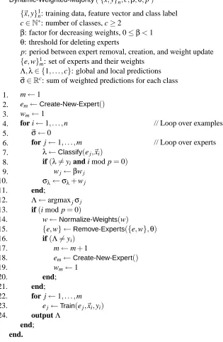
Figure 4: Number of experts maintained with 95% confidence intervals forDWM-NBandDWM-ITI on the STAGGERconcepts (Kolter and Maloof, 2003). c2003 IEEE Press. Used with permission.
step 40 for all three target concepts,DWM-NBperformed almost as well as naive Bayes with perfect forgetting.
DWM-ITI performed similarly, as shown in the right graph of Figure 3, achieving accuracies nearly as high as ITI with perfect forgetting. DWM-ITI converged more quickly than did DWM -NB to the second and third target concepts, but if we compare the plots for naive Bayes and ITI with perfect forgetting, we see that ITI converged more quickly to these target concepts than did naive Bayes. Thus, the faster convergence is due to differences in the base learners rather than to something inherent toDWM.
30 40 50 60 70 80 90 100
0 20 40 60 80 100 120
Predictive Accuracy (%)
Time Step (t) DWM-ITI
AQ-PM AQ11
30 40 50 60 70 80 90 100
0 20 40 60 80 100 120
Predictive Accuracy (%)
Time Step (t) DWM-ITI AQ11-PM AQ11-PM+WAH
Figure 5: Predictive accuracy with 95% confidence intervals on the STAGGER concepts. Left: DWM-ITI,AQ-PM, andAQ11. Right:DWM-ITI,AQ11-PM, andAQ11-PM+WAH.
20 30 40 50 60 70 80 90 100
0 20 40 60 80 100 120
Predictive Accuracy (%)
Time Step (t) DWM-ITI DWM-NB STAGGER
20 30 40 50 60 70 80 90 100
0 20 40 60 80 100 120
Predictive Accuracy (%)
Time Step (t) DWM-ITI DWM-NB Blum’s Weighted Majority
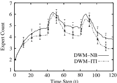
Figure 6: Predictive accuracy with 95% confidence intervals on the STAGGER concepts. Left: DWM-ITI, DWM-NB, and STAGGER. Right: DWM-ITI, DWM-NB, and Blum’s weighted majority (Kolter and Maloof, 2003). c2003 IEEE Press. Used with permission.
made more mistakes than did ITI, DWM-NBcreated more experts than didDWM-ITI. We can also see in the figure that the rates of removing experts were roughly the same for both learners.
The left graph of Figure 5 compares the performance of DWM-ITI to that of AQ-PM (Maloof and Michalski, 2000) and AQ11 (Michalski and Larson, 1983). DWM-ITI andAQ-PMperformed similarly on the first target concept, butDWM-ITIsignificantly outperformedAQ-PMon the second and third concepts, again, in terms of asymptote and slope. AQ11, although not designed to cope with concept drift, outperformedDWM-ITIin terms of asymptote on the first concept and in terms of slope on the third, but on the second concept, performed significantly worse than didDWM-ITI.
The left graph of Figure 6 compares the performance of our learners to that of our implemen-tation ofSTAGGER(Schlimmer, 1987). Comparing to bothDWMlearners,STAGGER’s performance was only slightly better on the first target concept, notably worse on the second, and comparable on the third.
Finally, the right diagram of Figure 6 shows the results from the experiment involving Blum’s (1997) implementation of weighted majority, the implementation that uses pairs of features as ex-perts. This learner outperformed DWM-NB and DWM-ITI on the first target concept, performed slightly worse on the second, and performed considerably worse on the third.
With respect to complexity of the experts themselves, the STAGGER concepts consist of three attributes, each taking one of three possible values. Therefore, this implementation of weighted ma-jority maintained 27 experts throughout the presentation of examples, as compared to the maximum of six thatDWM-NBmaintained. Granted, pairs of features and their recent predictions are much simpler than the decision trees thatITI produced, but naive Bayes was quite efficient, maintaining twenty-one integers for each expert. There were occasions when Blum’s weighted majority used less memory than didDWM-NB, but we anticipate that using more sophisticated classifiers, such as naive Bayes, instead of all combinations of pairs of features, will lead to scalable algorithms.
We focus our analysis onDWM-ITI, since it performed better than didDWM-NBon this problem. Researchers have built several systems for coping with concept drift and have evaluated many of them on theSTAGGER concepts. FLORA2 (Widmer and Kubat, 1996) is a prime example, and on the first target concept,DWM-ITIdid not perform as well as didFLORA2. However, on the second and third target concepts,DWM-ITIperformed notably better than didFLORA2, not only in terms of asymptote, but also in terms of slope.
DWM-ITIoutperformed AQ-PM(Maloof and Michalski, 2000), which had difficulty acquiring the second and third concepts (see Figure 5). AQ-PMmaintains examples over a fixed window of time and, at each time step, relearns concepts from these and new examples. In this experiment, when the concept changed from the first to the second, the examples of the first concept remaining in this window preventedAQ-PMfrom adjusting quickly to the second. Decreasing the size of this window improved accuracy on the second concept, but negatively affected performance on the third. Compared toDWM-ITI,AQ11 performed poorly on the second concept, but performed excep-tionally well on the third concept. Our analysis suggests that its poor performance on the second concept was because of AQ11’s expressive language for representing concepts. Notice that all of its rules achieved 100% on the first concept (see Figure 5, left). However,AQ11 produced twelve different rules for the first concept over the fifty runs. Some rules were similar, but others were quite different. AQ11 modifies its rules using only new examples, and in some cases, was able to transform rules for the first concept into rules with high accuracy on the second. Indeed, when we trained AQ11 only on examples of the second concept, it achieved 97%. However, in some trials, AQ11 was unable to make the required transformation and failed to learn adequately the second concept. We contend that ifAQ11 produced simpler rules, provided that they were the right ones, it would have performed much better on the second concept. Indeed, it is well known that simpler models often perform better than do more complex ones.
concept descriptions. When new examples arrive, AQ11-PMlearns incrementally from these new examples and those present in the window. Although the presence of these examples may have decreased AQ11’s (i.e.,AQ11-PM’s) performance on the third concept, their presence notably im-proved its performance on the second concept. If our hypothesis is correct—thatAQ11 would have performed better had it produced simpler models—the examples held in the window may have con-strainedAQ11 such that it produced simpler models. Put another way, the examples in the window reduced the instability of the learner. We found this discovery intriguing and plan to investigate it in future work.
STAGGER(Schlimmer and Granger, 1986) performed comparably toDWM-ITI on the first and third target concepts, but did not perform as well as DWM-ITI on the second target concept. (See Figure 6, left.) Generally, acquiring the second concept after learning the first is the hardest task, as the second concept is almost a reversal of the first; the two concepts share only one positive example. Acquiring the third concept after acquiring the second is easier because the two concepts share a greater number of positive examples. Performing well on the second concept therefore requires quickly disposing of knowledge and perhaps examples of the first target concept. A learning method, such as STAGGER, that only refines concept descriptions will have more difficulty responding to concept drift, as compared to an ensemble method, such asDWM, that both refines existing concept descriptions and creates new ones.
ComparingDWM-ITIto Blum’s weighted majority,DWM-ITI outperformed it on theSTAGGER concepts. However, our analysis suggests that the difference in performance is due to the experts, rather than to the global algorithms. Recall that Blum’s weighted majority uses as experts pairs of features with a brief history of past predictions. For the STAGGER concepts, pairs of features are useful for acquiring the first target concept (see Figure 2), which is conjunctive. Indeed, pairs of features are two-term conjunctions. However, the second and third concepts are disjunctive, and these are difficult to represent using only weighted pairs of features. As a result, on theSTAGGER concepts, Blum’s weighted majority did not perform as well asDWM.
Overall, we concluded that DWM-ITI outperformed these other learners in terms of accuracy, both in slope and asymptote. In reaching this conclusion, we gave little weight to performance on the first concept, since most learners can acquire it easily and doing so requires no mechanisms for coping with drift. On the second and third concepts, with the exception of AQ11, DWM-ITI performed as well or better than did the other learners. And whileAQ11 outperformedDWM-ITIin terms of slope on the third concept, this does not mitigateAQ11’s poor performance on the second.
70 75 80 85 90 95 100
0 12500 25000 37500 50000
Predictive Accuracy (%)
Time Step (t) Naive Bayes NB w/ Perfect Forgetting DWM-NB
Time Step (t)
50000 37500
25000 12500
0 0 10 20 30 40 50
Expert Count
DWM−NB, 10% Class Noise DWM−NB, No Noise
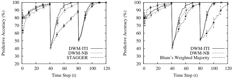
Figure 7: Performance with 95% confidence intervals ofDWM-NBon theSEA concepts with 10% class noise (Kolter and Maloof, 2003). Left: Predictive accuracy. Right: Number of experts maintained. c2003 IEEE Press. Used with permission.
4.2 Performance on a Larger Data Set with Concept Drift
To determine how wellDWM-NBperforms on larger problems involving concept drift, we evaluated it using a synthetic problem recently proposed in the data mining community (Street and Kim, 2001). This problem, which we call the “SEA concepts”, consists of three attributes, xi∈Rsuch
that 0.0≤xi ≤10.0. The target concept is x1+x2≤b, where b∈ {7,8,9,9.5}. Thus, x3 is an irrelevant attribute.
The presentation of training examples lasts for 50,000 time steps. For the first fourth (i.e., 12,500 time steps), the target concept is with b=8. For the second, b=9; the third, b=7; and the fourth, b=9.5. For each of these four periods, we randomly generated a training set consisting of 12,500 examples. In one experimental condition, we added 10% class noise; in another, we did not, and this latter condition served as our control. We also randomly generated 2,500 examples for testing. At each time step, we presented each method with one example, tested the resulting concept descriptions using the examples in the test set, and computed the percent correct. We repeated this procedure ten times, averaging accuracy over these runs. We also computed 95% confidence intervals.
On this problem, we evaluatedDWM-NB, naive Bayes, and naive Bayes with perfect forgetting. We setDWM-NBto halve the expert weights (i.e.,β=0.5) and to update these weights and to create and remove experts every fifty time steps (i.e., p=50). We set the algorithm to remove experts with weights less than 0.01 (i.e.,θ=0.01).
In the left graph of Figure 7, we see the predictive accuracies for DWM-NB, naive Bayes, and naive Bayes with perfect forgetting on theSEAconcepts with 10% class noise. As with theSTAGGER concepts, naive Bayes performed the worst, since it had no direct method of removing outdated concept descriptions. Naive Bayes with perfect forgetting performed the best and represents the best possible performance for this implementation on this problem. Crucially, DWM-NB achieved accuracies nearly equal to those achieved by naive Bayes with perfect forgetting.
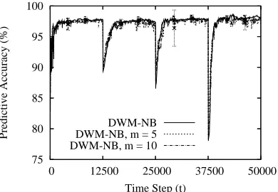
75 80 85 90 95 100
0 12500 25000 37500 50000
Predictive Accuracy (%)
Time Step (t) DWM-NB DWM-NB, m = 5 DWM-NB, m = 10
Figure 8: Predictive accuracy with 95% confidence intervals forDWM-NBon theSEAconcepts with 10% class noise. The number of experts was capped at five and at ten and compared to DWM-NBwith no limit on the number of experts created.
example. In the noisy condition, since 10% of the examples had been relabeled, DWM-NB made more mistakes and therefore created more experts than it did in the condition without noise.
As mentioned previously, DWMhas the potential for creating a large number of experts, espe-cially in noisy domains, since it creates a new expert every time the global prediction is incorrect. (The parameter p can help mitigate this effect.) A large number of experts obviously impacts mem-ory utilization, and, depending on the complexity of the base learners, could also affect learning and performance time, sinceDWMtrains and queries each expert in the ensemble when a new example arrives. An obvious scheme when resources are constrained is to limit the number of experts that DWMmaintains.
To investigate this strategy’s effect onDWM’s performance, we produced a version of the algo-rithm that always keeps the k best performing experts. That is, after reaching the point where there are k experts in the ensemble, whenDWMadds a new expert, it removes the expert with the lowest weight. In this version ofDWM, we set the threshold for removing experts to zero, which guaranteed that experts were removed only if they were the weakest member of the ensemble of k experts.
We ran this modified version on theSEAconcepts, capping the number of experts at five and at ten. We present these results in Figure 8. As one can see, for this problem, restricting the number of experts did not appreciably impact performance. Indeed,DWM-NBwith five experts performed almost as well as the original algorithm that placed no limit on the number of experts created.
Comparing our results for theSEAconcepts to those reported by Street and Kim (2001),DWM -NB outperformed SEA on all four target concepts. On the first concept, performance was similar in terms of slope, but not in terms of asymptote, and on subsequent concepts,DWM-NBconverged more quickly to the target concepts and did so with higher accuracy. For example, on concepts 2–4, just prior to the point at which concepts changed,SEA achieved accuracies in the 90–94% range, whileDWM-NB’s were in the 96–98% range.
is added, provided the ensemble does not contain a maximum number of classifiers; otherwise,SEA replaces a poorly performing classifier in the ensemble with the new classifier.
However, if every classifier in the ensemble has been trained on a given target concept, and the concept changes to one that is disjoint, thenSEA must replace at least half of the classifiers in the ensemble before accuracy on the new target concept will surpass that on the old. For instance, if the ensemble consists of 20 classifiers, and each learns from a fixed set of 500 examples, then it would take at least 5,000 additional training examples before the ensemble contained a majority number of classifiers trained on the new concept.
In contrast,DWMunder similar circumstances requires only 1,500 examples. Assume p=500, the ensemble consists of 20 fully trained classifiers, all with a weight of one, and the new concept is disjoint from the previous one. When an example of this new concept arrives, all 20 classifiers will predict incorrectly,DWMwill reduce their weights to 0.5—since the global prediction is also incorrect—and it will create a new classifier with a weight of one. It will then process the next 499 examples.
Assume another example arrives. The original 20 experts will again misclassify the example, and the new expert will predict correctly. Since the weighted prediction of the twenty will be greater than that of the one, the global prediction will be incorrect, the algorithm will reduce the weights of the twenty to 0.25, and it will again create a new expert with a weight of one. DWMwill again process 499 examples.
Assume a similar sequence of events occurs: another example arrives, the original twenty mis-classify it, and the two new ones predict correctly. The weighted-majority vote of the original twenty will still be greater than that of the new experts (i.e., 20(0.25)>2(1)), soDWMwill decrease the weight of the original twenty to 0.125, create a new expert, and process the next 499 examples. However, at this point, the three new classifiers trained on the target concept will be able to overrule the predictions of the original twenty, since 3(1)>20(0.125). Crucially,DWMwill reach this state after processing only 1,500 examples.
Granted, this analysis ofSEAandDWMdoes not take into account the convergence of the base learners, and as such, it is a best-case analysis. The actual number of examples required may be greater for both to converge to a new target concept, but the relative proportion of examples should be similar. This analysis also holds if we assume thatDWMreplaces experts, rather than creating new ones. Generally, ensemble methods with weighting mechanisms, like those present inDWM, will converge more quickly to target concepts (i.e., require fewer examples) than will methods that replace unweighted learners in the ensemble.
Regarding the number of experts thatDWMmaintained, we used a simple heuristic that added a new expert whenever the global prediction was incorrect, which intuitively, should be problematic for noisy domains. However, on the SEA concepts, while DWM-NB maintained as many as 40 experts at, say, time step 37,500, it maintained only 22 experts on average over the 10 runs, which is similar to the 20–25 thatSEAreportedly stored (Street and Kim, 2001).
If the number of experts were to reach impractical levels, thenDWMcould simply stop creating experts after obtaining acceptable accuracy; training would continue. Plus, we could easily dis-tribute the training of experts to processors of a network or of a course-grained parallel machine. And as the results pictured in Figure 8 demonstrate, we can limit the number of experts thatDWM maintains with potentially little effect on accuracy.
naive Bayes as the base learner. We refuted this hypothesis by running both base learners on each of the four target concepts. Both achieved comparable accuracies on each concept. For example, on the first target concept, C4.5 achieved 99% accuracy and naive Bayes achieved 98%. Since these learners performed similarly, we concluded that our positive results on this problem were due not to the superiority of the base learner, but to the mechanisms that create, weight, and remove experts.
We did not evaluate DWM-ITI on theSEA concepts, since ITI maintains all training examples and all observed values for continuous attributes, and this would have led to impractical memory requirements. However, this does not exclude the possibility of usingDWMon large data sets with a decision-tree learner as the base algorithm. For instance, we could useITI, but implement schemes to index stored training examples, which would reduce memory requirements. We could also use a decision-tree learner that does not store examples, such asID4 (Schlimmer and Fisher, 1986) or VFDT(Domingos and Hulten, 2000).
4.3 Calendar Scheduling Domain
The Calendar Apprentice (CAP) predicts user preferences for scheduling meetings in an academic institution (Mitchell et al., 1994). The task is to predict a user’s preference for a meeting’s location, duration, starting time, and day of the week. The data set consists of 34 features—such as the type of meeting, the purpose of the meeting, the type of attendees, and whether the meeting occurs during lunchtime—with intersecting subsets of these features for each prediction task. There are 12 features for location, 11 for duration, 15 for start time, and 16 for day of week. Although data are available for two users, we used the 1,685 examples of the preferences for User 1 (Tom Mitchell).
For this experiment, we evaluated naive Bayes andDWM-NB. However, unlike previous designs, in which we tested the resulting classifiers using a test set, in this design, we measured performance on the next example (i.e., the next meeting to be scheduled). For this application, when another user proposes a meeting, the Calendar Apprentice predicts, say, the meeting’s location, and the user either accepts or rejects the recommendation. The learner then uses this feedback to update its model of the user’s preferences.
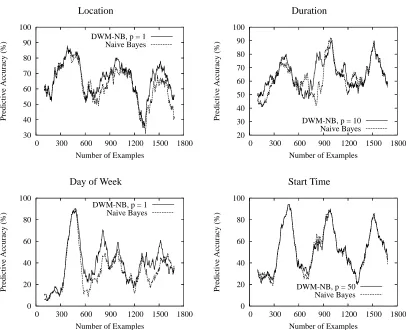
Table 1 shows the average performance of naive Bayes andDWM-NBfor the calendar schedul-ing task. With the exception of predictschedul-ing the preferred day of week for meetschedul-ings,DWM-NB outper-formed naive Bayes. Over the four prediction tasks,DWM-NBoutperformed naive Bayes. As one can see, increasing the parameter p, which governs how oftenDWMupdates its experts, generally decreasedDWM’s performance. Figure 9 shows accuracy versus the number of examples for the two learners on the four prediction tasks. According to Blum (1997), the sharp decreases in accuracy roughly correspond to the boundaries of semesters.
On this problem, Blum (1997) reported that, over the four prediction tasks, the CAP system averaged 53% and weighted majority with pairs of features averaged 57%. (Other algorithms in this study, such as winnow, performed even better.) DWM-NBaveraged about 55%, which was better than the originalCAPsystem, which used a decision tree to predict, but it was not better than Blum’s weighted majority.
DWM-NB
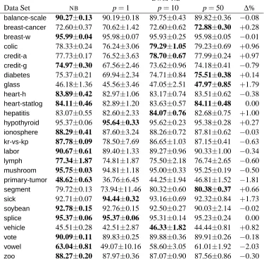
Prediction Task Naive Bayes p=1 p=10 p=50 Location 62.14 65.69 65.16 62.43 Duration 62.37 64.44 64.62 63.03 Start Time 32.40 38.10 37.39 34.96 Day of Week 51.22 51.16 49.13 51.34
Average 52.03 54.85 54.07 52.84
Table 1: Percent correct of naive Bayes andDWM-NBon the CAPdata set, using 1,685 examples for User 1. The variance of 1,685 Bernoulli trials is 0.0144%.
Location Duration
30 40 50 60 70 80 90 100
0 300 600 900 1200 1500 1800
Predictive Accuracy (%)
Number of Examples DWM-NB, p = 1 Naive Bayes
20 30 40 50 60 70 80 90 100
0 300 600 900 1200 1500 1800
Predictive Accuracy (%)
Number of Examples DWM-NB, p = 10
Naive Bayes
Day of Week Start Time
0 20 40 60 80 100
0 300 600 900 1200 1500 1800
Predictive Accuracy (%)
Number of Examples DWM-NB, p = 1
Naive Bayes
0 20 40 60 80 100
0 300 600 900 1200 1500 1800
Predictive Accuracy (%)
Number of Examples DWM-NB, p = 50
Naive Bayes
50 60 70 80 90 100
0 10000 20000 30000 40000 50000
Predictive Accuracy (%)
Time Step (t) Naive Bayes DWM-NB, p = 1
14 16 18 20 22 24 26 28 30
0 10000 20000 30000 40000 50000
Number of Experts
Time Step (t)
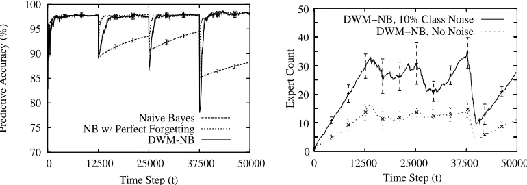
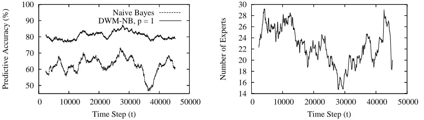
Figure 10: Performance ofDWM-NBon the electricity pricing task. Measures are averages of the previous 2,352 predictions. Left: Predictive accuracy. Right: Number of experts main-tained.
conditionally-dependent attributes, and we suspect that this is why Blum’s (1997) implementation of weighted majority outperformedDWM-NBon this problem.
Since Blum’s implementation forms concept descriptions consisting of weighted pairs of at-tribute values, we reasoned that conditionally-dependent atat-tributes would have less affect on its per-formance than they would on naive Bayes’. Indeed, experts that predict based on pairs of attribute values should benefit from conditionally-dependent attributes. Furthermore, since the weighting scheme identifies sets of predictive pairs of attribute values, it should do so regardless of condi-tional dependence among those attributes.
4.4 Electricity Pricing Domain
As a second evaluation on a real-world problem, we selected the domain of electricity pricing (Har-ries, 1999; Gama et al., 2004). Harries (1999) obtained this data set from TransGrid, the electricity supplier in New South Wales, Australia. It consists of 45,312 instances collected at 30-minute in-tervals between 7 May 1996 and 5 December 1998.1 Each instance consists of five attributes and a class label of eitherupordown. There are two attributes for time: day of week, which is an integer in[1,7], and period of day, which is an integer in[1,48](since there are 48 thirty-minute periods in one day). The remaining three attributes are numeric and measure current demand: the demand in New South Wales, the demand in Victoria, and the amount of electricity scheduled for transfer be-tween the two states. The task is to use the attribute values to predict whether the price of electricity will go up or down.
Since predicting the price of electricity is an online task, we processed the examples in temporal order—the order they appeared in the data set. For each example, we first obtained predictions from DWM-NB and from naive Bayes, and then trained each learner on the example. (This is the same experimental design we followed for the calendar scheduling task.) As before, we setDWMto halve expert weights (β=0.5), to update each time step (p=1), and to remove an expert if its weight falls below 0.01 (θ=0.01).
Overall, naive Bayes averaged 62.32% andDWM-NBaveraged 80.75%, maintaining an average of 22 experts. For reference, Harries (1999) used an online version of C4.5 (Quinlan, 1993) that
built a decision tree from examples in a sliding window and then classified examples in the following week, reporting accuracies for various window sizes between 66% and 67.7%.
In Figure 10, we present performance curves for accuracy and for the number of experts that DWMmaintained. To produce these curves, we averaged the raw performance metrics over a one-week period (i.e., 2,352 observations).
As a data set derived from real-world phenomenon, we cannot know definitively if or when concept drift occurred. Nonetheless,DWMdoes appear to have been more robust to change present in the samples than was naive Bayes. One example is the period surrounding time step 10,000. Naive Bayes’ predictive accuracy fluctuates during this period, butDWM’s remains nearly constant, on average.
Most illustrative is naive Bayes’ sudden drop of roughly 12% in accuracy between time steps 35,000 and 37,000. DWM’s accuracy decreased slightly and steadily during this period, but there was no comparable sudden decrease in performance.
The number of experts that DWM maintained fluctuated considerably between 1 and 90, but with an overall average of 22 experts. In terms of the weekly average, shown in the right graph of Figure 10, the average size of the ensemble never exceeded 29 experts, which we found encouraging for a problem with 45,312 examples.
4.5 Evaluation on Static Concepts
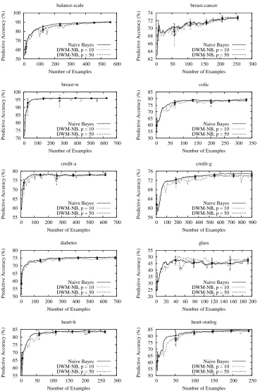
Finally, we evaluatedDWM-NBon 26 data sets from the UCI Repository (Asuncion and Newman, 2007). It is clear that, for static concepts, there is nothing inherent to theDWMalgorithm that would make it more advantageous than a single learner. However, it is important to establish that DWM performs no worse than a single learner. Therefore, we selected data sets that varied in the number of classes, the number of examples, the types of attributes, and the number of missing values.
For each data set, we randomly selected 10% of the examples for testing.2 We presented each example of the remaining 90% to naive Bayes and toDWM-NBwith three settings of the parameter
p: 1, 10, and 50. After each presentation, we evaluated the resulting concept descriptions on the
examples in the testing set. We repeated this procedure ten times, averaging percent correct over these runs and computing 95% confidence intervals.
The results, presented in Appendix A, demonstrate thatDWM-NBperformed no worse than naive Bayes, the single base learner. As one can see in Table 2, naive Bayes outperformedDWM-NBon most of the tasks (16 of 26), but many of these differences are within 0.5%. For the tasks on which DWM-NBoutperformed naive Bayes, many of the differences in performance were also within this range. Overall, the average difference in performance is+0.35%—in DWM’s favor—and so we concluded that, on these data sets, DWM-NB performed no worse than a single instance of naive Bayes.
In Figures 11–13, we present the learning curves for this experiment. For legibility, we did not include the curves forDWM-NBwith p=1. LimitingDWM-NBto ten experts reduced performance only slightly, and we omitted these results for brevity.
5. Concluding Remarks
Tracking concept drift is important for many applications. Clearly, with learners for drifting con-cepts, there is a balance between learning that is completely reactive (e.g., predicting based only on the last example) and learning that is completely unreactive (e.g., predicting based on all encoun-tered examples). If a learner knew when concepts had changed, it could discard its old descriptions and start learning anew. However, this may not always lead to optimum performance on a task be-cause there may be knowledge of the old concept useful for acquiring the new concept. If the learner could appropriately leverage its relevant old knowledge, then performance on the new concept may be better, if not in terms of asymptote, then perhaps in terms of slope.
In this paper, we presented an ensemble method based on the weighted majority algorithm (Lit-tlestone and Warmuth, 1994). Our method, dynamic weighted majority, creates and removes base algorithms in response to changes in performance, which makes it well suited for problems involv-ing concept drift. We described two implementations of DWM, one with naive Bayes as the base learner, the other withITI(Utgoff et al., 1997). On the problems we considered, a weighted ensem-ble of learners with mechanisms to add and remove experts in response to changes in performance provided a better response to concept drift than did other learners, especially those that relied on only incremental learning (i.e.,STAGGERandAQ11), on the maintenance of previously encountered examples (i.e., FLORA2 and the AQ-PMsystems), or on an ensemble of unweighted learners (i.e., SEA).
Using the STAGGER concepts, we evaluated DWM-NB and DWM-ITI our implementation of STAGGER, Blum’s implementation of weighted majority, and four rule learners based on the AQ algorithm. To determine performance on a larger problem, we evaluatedDWM-NBon theSEA con-cepts. Results on these problems, when compared to other methods, suggest thatDWMmaintained a comparable number of experts, but achieved higher predictive accuracies and converged to those accuracies more quickly. Indeed, to the best of our knowledge, these are the best overall results reported for these problems.
DWM, on a calendar scheduling task, outperformed theCAPsystem and performed comparably to Blum’s weighted majority. On an electricity pricing domain, DWMoutperformed a single base learner and an online version of C4.5 (Harries, 1999). Finally, on several problems with static concepts,DWMperformed as well as a single base learner.
In future work, we plan to investigate more sophisticated heuristics for creating new experts: Rather than creating an expert when the global prediction is wrong, perhapsDWMshould take into account the expert’s age or its history of predictions. We would also like to investigate another decision-tree learner as the base algorithm, one that does not maintain encountered examples and that does not periodically restructure its tree;VFDT(Domingos and Hulten, 2000) is a likely candi-date.
Although removing experts of low weight yielded positive results for the problems we consid-ered in this study, it would be beneficial to investigate mechanisms for explicitly handling noise, such as those present inIB3 (Aha et al., 1991), or for determining when examples are likely to be from a different target concept, such as those based on the Hoeffding (1963) bounds present inVFDT (Domingos and Hulten, 2000) andCVFDT(Hulten et al., 2001).
af-fects a learner’s stability and its ability to cope in non-stationary environments. We anticipate that these investigations will lead to general, robust, and scalable ensemble methods for tracking concept drift.
Acknowledgments
The authors thank Dale Schuurmans, William Headden, and the anonymous reviewers for helpful comments on earlier drafts of the manuscript. We thank Avrim Blum and Paul Utgoff for releasing their respective systems to the research community. We also thank Jo ˜ao Gama for providing the data set for electricity pricing, and Michael Harries for its original distribution. This research was conducted in the Department of Computer Science at Georgetown University. The work was sup-ported in part by the National Institute of Standards and Technology under grant 60NANB2D0013 and byGUROP, the Georgetown Undergraduate Research Opportunities Program. The authors are listed in alphabetical order.
Appendix A. Performance ofDWM-NBon SelectedUCIData Sets