R E S E A R C H
Open Access
Boundary value problems on part of a
level-n Sierpinski gasket
Xuliang Li
**Correspondence: [email protected] Department of Mathematical Sciences, Tsinghua University, Beijing 100084, China
Abstract
We study the boundary value problems for the Laplacian on a sequence of domains constructed by cutting level-n Sierpinski gaskets properly. Under proper assumptions on these domains, we manage to give an explicit Poisson integral formula to obtain a series of solutions subject to the boundary data. In particular, it is proved that there exists a unique solution continuous on the closure of the domain for a given sequence of convergent boundary values.
MSC: 28A80; 35J25
Keywords: boundary value problems; level-n Sierpinski gasket; harmonic functions; postcritically finite; fractal Laplacian
1 Introduction
The study of boundary value problems on the domains of Sierpinski gasket (SG) was initi-ated by []. Since then, two natural choices have been considered, namely the upper part of SG cut by a horizontal line (cf. [, ]) and half Sierpinski gasket constructed by cutting SG with a vertical line in the middle (cf. []). For more related works see, for example, [–]. This work is strongly motivated by [].
In this work, we will introduce a new class of domains on level-n Sierpinski gasket and prove the exact form of the solution to the boundary value problems on these domains. Note that these domains are new examples of non-p.c.f. (postcritically finite) type fractals (can also be viewed as fractafold in [, ]) where harmonic functions can be well defined. We follow [, ] by recalling that the fractalKis the invariant set for a finite iterated function systems (IFS) of contractive similarities in the Euclidean spaceR. We denote the mappings{Fi}i=,....N–for some positive integerN. ThenK is the unique nonempty compact set satisfying
K= N–
i=
Fi(K). (.)
Form≥, we define the space of words of lengthmby
WmN={, , , . . . ,N– }m=ww. . .wm:wi∈ {, , , . . . ,N– }
.
w∈WN
m is called a word of lengthmwith symbols{, , , . . . ,N– }. We also setW∗N=
m≥WmN and denote the length ofw∈W∗N by|w|.
Recall thatKis calledpostcritically finite(p.c.f.) ifKis connected and there exists a finite setV⊆Kcalled theboundarysuch that
FwK∩FwK⊆FwV∩FwV forw=wwith|w|=w, (.) with the intersection disjoint fromV. SetV={q,q, . . . ,qN}forN<N. We require that each boundary point is the fixed point of one of the mappings{Fi}and that
Fi(qi) =qi for ≤i≤N. (.)
The standard SG is the unique nonempty compact setKsatisfying (.) with the bound-ary setV={q,q,q}, where the contractive mappings{Fi}i=,,are given by
Fi(x) =
(x–qi–) +qi–.
Similarly, thelevel- Sierpinski gasketSGis the unique nonempty compact setK satisfy-ing (.) with the boundary setV={q,q,q}, where{Fi}i=...,are given by
Fi(x) =
(x–qi) +qi. (.)
Hereq=q+q,q=q+q,q=q+q. See Figure for an illustration. As above, we can definelevel-n Sierpinski gasketin a similar way.
Inspired by [] we will construct a new class of domains in the following statement.
1.1 Description of the general domains
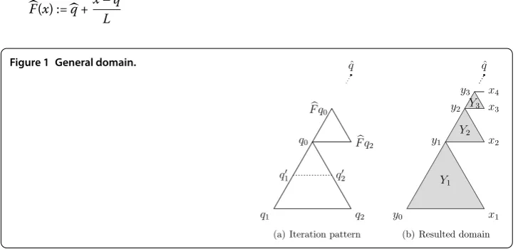
LetK= SGnandK˜ =nK, that is, shrinkingK ntimes. Denote byEthe compact triangular domain with boundary set{q,q,q}which is constructed by gluing finite copies ofK˜ at boundary (see Example . below). Assume that the compact triangular domainE with boundary{q,q,q}(as a part ofE) satisfiesE=F(E), whereF(x) :=q+x–Lq for some constantL(see Figure (a)). Pick some pointqˆsuch that the contractive map
F(x) :=q+x–q
L
satisfiesF(q) =q. SetE=E\{q,q},y=q,ym=Fm(q),xm=Fm–(q),Ym:=Fm–(E) for integerm> (see Figure (b)). LetX=∞m={xm}. Set
∂Ym={ym–,ym,xm}, Ym=Ym∪∂Ym. For eachYmdefine mappingFmas
Fm(z) =ym+
z–ym
L . (.)
Then by assumptionYmis self-similar with respect toFm. Define
:=
∞
m=
Ym, :=
∞
m=
Ym. (.)
We say that the setis a DCPB(domain of countable-point boundary)with boundary
∂:=X∪y∪ ˆqforK= SGn.
Remark . In application, we need the constantL=nk withk> to ensure thatEis self-similar with respect to the mapF, and thusFm(Ym) is exactly a copy ofYm+. This property is useful in constructing harmonic functions on these domains in a sequel. The description of those domains will be justified by the examples below.
1.2 Examples
Example . ForK= SG, letE=F(K) be the compact triangular domain with boundary set{q,p,p}(see Figure ). LetE=E/{q,p}, sety=q,ym=F(q),xm=Fm–(p) and
Ym=Fm–(E) for all positive integersm, whereFis as defined in (.). SetF=F,qˆ=q. Then(green part) can be well established as in (.) .
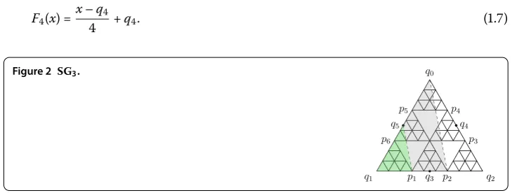
Example . ForK= SG,E=F(K)∪F(K)∪F(K) is the compact triangular domain with boundary set{q,p,p} (see Figure ). LetE=E/{q,p}, sety=q,ym=Fm(q),
xm =Fm–(p) andYm =Fm–(E) for all positive integersm. LetX=
∞
m={xm}. Setting
F=F,qˆ=q, we obtain(gray part) as a DCPB by (.).
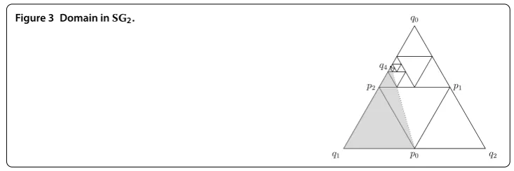
Example . ForK= SG,E=F(K) is the compact triangular domain with boundary points{q,p,p}(see Figure ). Letq=p+q and define the contractive mapping
F(x) =
x–q
+q. (.)
Figure 3 Domain inSG2.
LetE=E/{q,p}, sety=q,ym=Fm(q),xm=Fm–(p) andYm=Fm–(E) for allm> . LetX=∞m={xm}. SetF=F,qˆ=q. Now we can define the desired domainby (.). Note thatFis not one of the contractive mappings for standard SG.
In the following section, we construct a solution to the boundary value problem using harmonic extension algorithm. Denote byC(U) the space of all continuous functions on some setU. We will see that the space ofC()-solutions to the boundary value problem is one-dimensional, but in general, the solution blows up atqˆ. We show that if the boundary data onXconverges, there exists a uniqueC()-solution.
2 Main results
The Laplacian on the standard SG was first constructed as a generator of a stochastic pro-cess by Goldstein [] and Kusuoka []. Kigami [, ] developed an analytical version of the Laplacian for SG, and then generalized it to any p.c.f. self-similar set (see [], Def-inition .., p.).
We now study the boundary value problems onas a DCPB defined in Section .:
⎧ ⎨ ⎩
u= on,
u(y) =a, u(xm) =am on∂,
(BVP)
where denotes the Kigami’s Laplacian forK= SGnwith respect to the standard self-similar measure,u:→Ris the unknown, and{am}∞m=is the boundary data. Note that the Laplacianhere is well defined for all cellsYm, hence the wholeby recalling that every cellYmofcan be viewed as a part ofK= SGnor gluing several copies of it.
Harmonic extension algorithm is the simplest tool for constructing harmonic functions subject to boundary value problems on SGn. In fact, we can apply this algorithm infinitely many times and obtain a function harmonic on SGn.
Using this, we will give an explicit solution to (BVP) based on the following assumption.
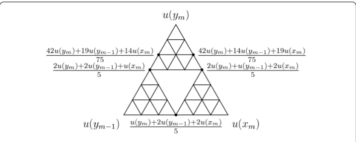
Assumption Letbe a DCPB forK= SGn. For each cellYmwith boundary set∂Ym= {ym–,ym,xm}, if some functionuis harmonic onYmand satisfies that
Figure 4 Values for Assumption 0 in Example 1.3.
for some real constantsc,c,c, then
⎡ ⎢ ⎣
u(ym)
u(ym–)
u(xm)
⎤ ⎥ ⎦=M
⎡ ⎢ ⎣
u(ym)
u(ym–)
u(xm)
⎤ ⎥ ⎦=M
⎡ ⎢ ⎣ c c c ⎤ ⎥
⎦, M=
⎡ ⎢ ⎣
θ θ θ
θ θ θ
⎤ ⎥
⎦ (.)
for some positive constantsθ,θ,θsatisfying that
θ+θ+θ= , (.)
whereym–=Fm(ym–),xm=Fm(xm) withFmgiven by (.).
Note that this assumption can be easily verified by harmonic extension algorithm. In Example ., we have (see Figure )
M=
⎡ ⎢ ⎣ ⎤ ⎥ ⎦.
We set, for Assumption ,
=θ+θ, = ( –θ),
T+=
+K
, T–=
–K
, K=
– .
Theorem . For every choice of the convergent boundary data{am}for someas a DCPB (defined in Section.)satisfying Assumption,there exists a one-dimensional space of C()solutions to the(BVP).For each real constantλ,there exists a unique solution to the
(BVP)uλsuch that uλ(y) =λand that uλ(xm) =amfor m≥.Furthermore,for m≥
uλ(ym) =K–
where
φ+m(λ) =λ–T+–(a+a) – (+T+) m
k=
T+–kak,
φ–m(λ) =λ–T––(a+a) – (+T–) m
k=
T––kak.
Proof For fixedm≥, letube a continuous piecewise harmonic function for (BVP). In view of Assumption , it is easy to adapt the argument for [], proof of Lemma ., to obtain thatu(ym) = holds if and only if
u(ym) =u(ym–) –u(ym–) –am–am–. (.) The rest is trivial algebra as in [], proof of Theorem ..
The theorem below can be obtained by following the argument in [], proof of Theo-rem ., Corollary .. We include a brief proof for the readers’ convenience.
Theorem . If am→A as m→ ∞for some constant A,there exists a unique solution to (BVP)u∈C()which satisfies that
u(y) =T+–(a+a) + (+T+)
∞
k=
T+–kak, (.)
and for m≥
u(ym) =K–(+T+)
∞
k=
T+–kam+k–T–m
∞
k=
T+–kak
+T–ma+a+K–(+T–) m
k=
T––kak
. (.)
Proof We first prove the theorem for the caseA= . Substituting (.) into (.) yields (.).
By using the triangle inequality, we have
u(ym)≤K–(+T+)
∞
k=
T+–k|am+k|–T–m
∞
k=
T+–k|ak|
+T–m
|a|+|a|+K–(+T–) m
k=
T––k|ak|
. (.)
From this andam→ we can easily see thatu(ym)→. Thus, by the definition of BVP, lim
m→∞u(xm) =mlim→∞u(ym) = .
For the caseA= , we consider the modified BVP:
⎧ ⎨ ⎩
u= on,
u(y) =a–A, u(xm) =am–A on∂.
Noting thatam–A→, the rest of the proof can be done by using the result from the last
part of the proof and the maximum principle.
Remark . The results in [], Section , reduce to a special case of our theorems above with parametersθ= /,θ= /,θ= /. Indeed, [] proved many more results on half SG. Many of them are highly dependent on the fact that we can obtain SG from half SG by reflection, and thus the top point enjoys many more nice properties than our domains. We will touch on that elsewhere.
Competing interests
The author declares that he has no competing interests.
Author’s contributions
The author read and approved the final manuscript.
Acknowledgements
The author is indebted to Professor Robert S. Strichartz for inviting them to work on this topic. The author is also grateful to Professor Jiaxin Hu for helpful comments on a draft version of the present work. This work was supported by the National Natural Science Foundation of China (11371217).
Publisher’s Note
Springer Nature remains neutral with regard to jurisdictional claims in published maps and institutional affiliations.
Received: 18 January 2017 Accepted: 28 March 2017
References
1. Owen, J, Strichartz, RS: Boundary value problems for harmonic functions on a domain in the Sierpinski gasket. Indiana Univ. Math. J.61(1), 319-335 (2012)
2. Guo, Z, Kogan, R, Qiu, H, Strichartz, RS: Boundary value problems for a family of domains in the Sierpinski gasket. Ill. J. Math.58(2), 497-519 (2014)
3. Li, W, Strichartz, RS: Boundary value problems on a half Sierpinski gasket. J. Fractal Geom.1(1), 1-43 (2014) 4. Bonanno, G, Bisci, GM, Radulescu, V: Existence results for gradient-type systems on the Sierpi ´nski gasket. Chin. Ann.
Math., Ser. B34(2), 941-953 (2013)
5. Bonanno, G, Molica Bisci, G, Radulescu, V: Infinitely many solutions for a class of nonlinear elliptic problems on fractals. C. R. Math. Acad. Sci. Paris350(3-4), 187-191 (2012)
6. Bonanno, G, Molica Bisci, G, Radulescu, V: Variational analysis for a nonlinear elliptic problem on the Sierpi ´nski gasket. ESAIM Control Optim. Calc. Var.18(4), 941-953 (2012)
7. Ferrara, M, Molica Bisci, G, Repovs, D: Existence results for nonlinear elliptic problems on fractal domains. Adv. Nonlinear Anal.5(1), 75-84 (2016)
8. Molica Bisci, G, Radulescu, V: A characterization for elliptic problems on fractal sets. Proc. Am. Math. Soc.143(7), 2959-2968 (2015)
9. Strichartz, RS: Fractafolds based on the Sierpi ´nski gasket and their spectra. Trans. Am. Math. Soc.355(10), 4019-4043 (2003)
10. Strichartz, RS: Fractals in the large. Can. J. Math.50(3), 638-657 (1998)
11. Kigami, J: Analysis on Fractals. Cambridge Tracts in Mathematics, vol. 143. Cambridge University Press, Cambridge (2001)
12. Strichartz, RS: Differential Equations on Fractals: A Tutorial. Princeton University Press, Princeton (2006)
13. Goldstein, S: Random walks and diffusions on fractals. In: Percolation Theory and Ergodic Theory of Infinite Particle Systems (Minneapolis, Minn., 1984-1985). IMA Vol. Math. Appl., vol. 8, pp. 121-129. Springer, New York (1987) 14. Kusuoka, S: Dirichlet forms on fractals and products of random matrices. Publ. Res. Inst. Math. Sci.25(4), 659-680
(1989)