International Doctorate School in Information and Communication Technologies
DISI - University of Trento
Optimal Adaptations over Multi-Dimensional Adaptation Spaces with a Spice of Control Theory
Konstantinos Angelopoulos
Advisor:
Prof. John Mylopoulos
Universit`a degli Studi di Trento
(Self-)Adaptive software systems monitor the status of their requirements and adapt when some of these requirements are failing. The baseline for much of the research on adaptive software systems is the concept of a feed-back loop mechanism that monitors the performance of a system relative to its requirements, determines root causes when there is failure, selects an adaptation, and carries it out. The degree of adaptivity of a software sys-tem critically depends on the space of possible adaptations supported (and implemented) by the system. The larger the space, the more adaptations a system is capable of. This thesis tackles the following questions: (a) How can we define multi-dimensional adaptation spaces that subsume proposals for requirements- and architecture-based adaptation spaces? (b) Given one of more failures, how can we select an optimal adaptation with respect to one or more objective functions?
To answer the first question, we propose a design process for three-dimensional adaptation spaces, named the Three-Peaks Process, that it-eratively elicits control and environmental parameters from requirements, architectures and behaviours for the system-to-be. For the second question, we propose three adaptation mechanisms. The first mechanism is founded on the assumption that only qualitative information is available about the impact of changes of the system’s control parameters on its goals. The absence of quantitative information is mitigated by a new class of require-ments, namely Adaptation Requirerequire-ments, that impose constraints on the adaptation process itself and dictate policies about how conflicts among failing requirements must be handled.
that the problem of finding an adaptation is formulated as a constrained multi-objective optimization problem. The mechanism measures the degree of failure of each requirement and selects an adaptation that minimizes it along with other objective functions, such as cost. Optimal solutions are de-rived exploiting OMT/SMT (Optimization Modulo Theories/Satisfiability Modulo Theories) solvers.
The third mechanism operates under the assumption that the environ-ment changes dynamically over time and the chosen adaptation has to take into account such changes. Towards this direction, we apply Model Predic-tive Control, a well-developed theory with myriads of successful applications in Control Theory. In our work, we rely on state-of-the-art system iden-tification techniques to derive the dynamic relationship between require-ments and possible adaptations and then propose the use of a controller that exploits this relationship to optimize the satisfaction of requirements relative to a cost-function. This adaptation mechanism can guarantee a certain level of requirements satisfaction over time, by dynamically com-posing adaptation strategies when necessary. Finally, each piece of our work is evaluated through experimentation using variations of the Meeting-Scheduler exemplar.
Keywords
This thesis is not only a result of hard work, but also an outcome of collaborating with many people during the years I have spent as PhD stu-dent. The shared experiences, thoughts and discussions I had with them, shaped me as a researcher and I am grateful to them for their contribution to my journey in the research world.
I would like to thank my advisor, John Mylopoulos, for his guidance and for teaching me how to approach a research problem. I am also thankful for sharing his experience in research with me and for all the good quality work we produced the past four and a half years.
I am also thankful to Vitor, with whom I collaborated closely all these years and his work constituted the baseline of my research. I would also like to thank Alessandro for his contribution to the last piece of this work and sharing with me his expertise in the fascinating field of Control Theory. I owe special thanks to both of you, as well as to Martina and Julio for accepting my invitation to participate in my thesis committee.
Thanks to my colleagues at the University of Trento for the numerous discussions, brainstormings, debates and seminars we shared, trying to make each other a better researcher and person. I wish our future will bring us again together collaborating, sharing ideas, pizzas and drinks. I am also very thankful to all my friends for their company all this time, the moments of joy and the experiences we shared.
Last, but not least, I would like to thank my parents for supporting me in every decision I have taken in my life. For standing by my side whenever I was in need or I wanted to share my happiness.
To all of you, thank you, grazie mille, ευχαριστω´!
1 Introduction 1
1.1 Challenges of complex software systems . . . 2
1.2 Software system adaptation . . . 5
1.2.1 Definitions . . . 5
1.2.2 Feedback Loops . . . 7
1.2.3 SISO and MIMO systems . . . 10
1.3 Objectives of our research . . . 11
1.3.1 Overview and contributions . . . 16
1.4 Structure of the thesis . . . 17
1.5 Published papers . . . 18
2 State of the Art 21 2.1 Baseline . . . 21
2.1.1 Goal Oriented Requirements Engineering . . . 22
2.1.2 GORE for self-adaptive software systems . . . 23
2.1.3 Requirements monitoring . . . 25
2.1.4 Variability in goal models . . . 28
2.1.5 Requirements Evolution . . . 29
2.1.6 Software Architecture Modelling . . . 31
2.1.7 Software Behaviour Modelling . . . 34
2.2 Dynamic System Modelling . . . 34
2.3.2 Architecture-based Adaptation . . . 39
2.3.3 Behaviour-based Adaptation . . . 41
2.3.4 Combined Model-based Adaptation . . . 42
2.3.5 Control-based Adaptation . . . 42
2.4 Chapter Summary . . . 44
3 Requirements and Architecture Approaches: A Compari-son 47 3.1 Selected Adaptation Approaches . . . 48
3.1.1 Rainbow . . . 49
3.1.2 Zanshin . . . 51
3.2 The ZNN.com Exemplar . . . 52
3.2.1 Overview of the problem and its architectural solution 53 3.2.2 An RE-based solution to ZNN.com using Zanshin . 56 3.3 Comparison between Rainbow and Zanshin . . . 61
3.3.1 Methodology . . . 62
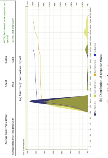
3.3.2 Experimental Results . . . 63
3.3.3 Discussion . . . 65
3.4 Chapter Summary . . . 69
4 Designing Adaptation Spaces 73 4.1 Capturing and exploring variability . . . 74
4.1.1 Variability in behaviour . . . 74
4.1.2 Variability in architecture . . . 79
4.1.3 Variability in the environment . . . 82
4.2 A Three-Peaks modelling process . . . 83
4.3 Evaluation . . . 87
5.1 Requirements for Adaptation . . . 94
5.1.1 Prioritizing Requirements . . . 94
5.1.2 Adaptation Requirements . . . 96
5.2 Adaptation Process for Multiple Failures . . . 101
5.3 Evaluation . . . 105
5.3.1 Meeting Scheduler Exemplar . . . 105
5.3.2 Improved Adaptation . . . 109
5.4 Chapter Summary . . . 110
6 The Next Adaptation Problem 113 6.1 Problem Formulation . . . 114
6.2 Prometheus Framework . . . 117
6.3 Evaluation . . . 120
6.3.1 The Meeting-Scheduler Exemplar . . . 120
6.3.2 The E-shop Exemplar . . . 126
6.3.3 Discussion . . . 130
6.4 Chapter Summary . . . 131
7 Control-based design of self-adaptive software 133 7.1 Model Predictive Control . . . 134
7.1.1 Formal description . . . 136
7.1.2 Formal guarantees . . . 139
7.2 Design phase . . . 141
7.3 Chapter Summary . . . 145
8 Control-based software adaptation 147 8.1 The CobRA framework . . . 148
8.2 Evaluation . . . 150
8.2.3 Discussion . . . 154 8.3 Chapter Summary . . . 157
9 Conclusions and future work 159
9.1 Contributions to the state-of-the-art . . . 160 9.2 Limitations of the approach . . . 165 9.3 Future work . . . 166
2.1 EvoReqs operations . . . 32
5.1 Pairwise Comparison Values . . . 95
5.2 Scale For Pairwise Comparisons . . . 97
5.3 Differential relations elicited for the Meeting Scheduler ex-ample [SLAM13] . . . 106
5.4 Priority Values of AwReqs . . . 107
5.5 Evoreq operations for AwReqs . . . 107
6.1 Control Parameter Profile. . . 115
6.2 Control Parameter Profile. . . 123
6.3 Control Parameter Profile. . . 127
7.1 Reference goals . . . 143
7.2 EvoReqs operations . . . 143
7.3 Indicator Priorities . . . 144
1.1 MAPE-K loop . . . 7
1.2 Feedback Loop . . . 8
1.3 SASO properties . . . 9
2.1 Goal model for the Meeting-Scheduler case study. . . 24
2.2 States assumed by requirements [SLRM11]. . . 25
2.3 Aggregate Awareness Requirements. . . 26
2.4 Trend Awareness Requirement. . . 27
2.5 Delta Awareness Requirement. . . 27
2.6 Goal model for the Meeting-Scheduler case study. . . 30
2.7 Architectural diagram for the Meeting-Scheduler . . . 33
3.1 The components of the Rainbow framework [Che08]. . . 50
3.2 An overview of the Zanshin approach [SS12]. . . 51
3.3 Znn.com architecture [CGS06b] . . . 53
3.4 Strategy SmarterReduceResponseTime in Stitch [Che08]. . 55
3.5 Goal model for the ZNN.com exemplar, mirroring the adap-tation scenarios modelled in Rainbow. . . 57
3.6 Specification of the SimpleReduceResponseTime strategy with Zanshin. . . 59
3.7 Specification of AR3 for the SmarterReduceResponseTime strategy. . . 61
expressions. . . 75
4.2 BCP from AND-refinement . . . 76
4.3 BCP from multiplicity operator . . . 78
4.4 BCP from OR-refinement . . . 79
4.5 ACP for component instance . . . 80
4.6 ACP for alternative component . . . 81
4.7 Domain model for the Meeting Scheduler environment . . . 83
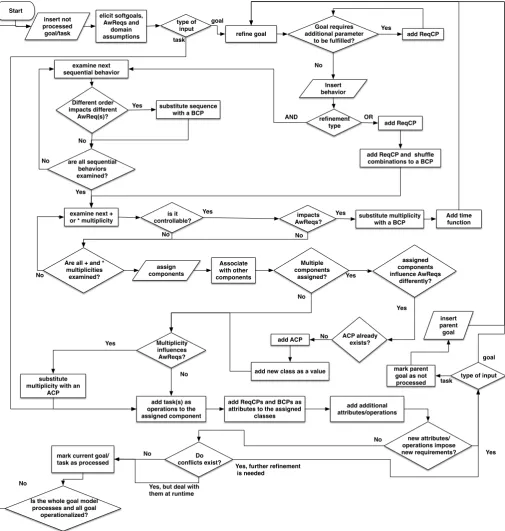
4.8 The Three-Peaks process as a flowchart . . . 84
4.9 The goal model after the Three-Peaks process . . . 89
4.10 The architecture model after the Three-Peaks process . . . 90
5.1 Adaptation Requirements Goal Model . . . 99
5.2 Zanshin Architecture . . . 101
5.3 Zanshin’s Adaptation Process . . . 103
5.4 Adaptation Requirements Goal Model [SS12] . . . 104
6.1 Goal model annotated with contributions . . . 115
6.2 Prometheus framework . . . 118
6.3 Meeting-Scheduler goal model . . . 121
6.4 E-shop goal model . . . 128
7.1 Control scheme. . . 139
7.2 Meeting Scheduler goal model . . . 142
8.1 CobRA framework . . . 148
8.2 Indicator measured values . . . 154
8.3 Control parameter values . . . 155
Introduction
There is nothing more difficult to take in hand, more perilous to conduct, or more uncertain in its success, than to take the lead in the
introduction of a new order of things.
Niccol`o Machiavelli
systems. Finally, we present and overview of this thesis’ proposal and contributions.
1.1
Challenges of complex software systems
As the environments of modern software systems become more dynamic, the level of uncertainty under which they operate increases dramatically. Therefore, software systems must be resilient to changes that can be fore-seen, foreseeable orunforeseen [Lap08]. For the latter case, a configuration management [KM90] mechanism has been proposed by Kramer and Magee to respond dynamically to changes in the environment, requirements or structure of the system. The baseline of this proposal is that an external mechanism should be able to reconfigure the software system by following a change management protocol that prescribes how to add, remove, link and unlink software modules, without causing any disruptions. This mech-anism should be independent of the particular application and its single objective is to maintain the system in a consistent state that is able to fulfil the system’s mandate.
components must coordinate in sometimes hostile environments to achieve common goals. Due to their size, replacement of such systems is impracti-cal in terms of cost and therefore when failures take place or requirements change, they must adapt. Another characteristic of ULS systems is that many different groups of stakeholders are involved and each of them has his or her own goals. Hence, trade-off mechanisms to satisfy all goals to a degree that corresponds to the importance of each group becomes essential. Similar to ULS, Ubiquitous Computing [Wei93] refers to a concept of software engineering where multiple networked devices collaborate to pro-vide various services. Applications of Ubiquitous Computing can be found in Smart Homes [EG01] and Smart Cities [CNW+12] that are designed in order to improve human daily tasks. The interconnected components of such environments may vary from smartphones, tablets to remote con-trolled house devices, all communicating with predefined protocols over a network. One of the main challenges in Ubiquitous Computing is that every user is unique, has his or her own goals and priorities. Therefore, the devices used by individuals in order to interact with their environment must adapt and be personalized. Moreover, user devices learn by time the habits and the preferences of the users providing them a better quality of service. Finally, as technology evolves, ubiquitous environments are popu-lated with new kinds of devices that need to communicate with the existing ones without interrupting their operation.
precision resource provisioning Virtual Machine (VM) migration in order to cope with unpredictable workload patterns and infrastructure failures. This mechanism must also balance conflicting objectives such as perfor-mance, operational cost and energy consumption and perform trade-offs that maximize the revenue of the provider and guarantee its reliability.
A new generation of systems, named Cyber Physical systems [Lee08] combine computational and physical capabilities. One of the main research challenges of this kind of systems is to guarantee a level of robustness in unknown environments by handling both software and physical failures. Given that Cyber Physical systems are destined also for mission critical operations, such as rescues in inaccessible locations, they must respond to changes and failures with high precision.
From the perspective of IT industry, multiple initiatives have provided solutions to many businesses. IBM’s Autonomic Computing presented in 2001 by Horn [Hor01] has been a point of reference for both academic and industrial research on the topic. This work is followed by Sun’s N1 manage-ment software [Sun], that was designed to tackle to problem of managing large, complex and heterogeneous infrastructures. Microsoft with its Dy-namic Software Initiative [Mic] contributed to a cost-effective automatic resource allocation in order to meet the growing demands of the market. At the same time Hewllett-Packard introduced the Adaptive Enterprise Strategy approach while Intel proposed standards for implementing auto-nomic computing solutions [TM06].
must include techniques and guidelines from other fields such as Control Theory, Mathematical Optimization, Artificial Intelligence, Formal Meth-ods and others, in order implement effective decision-making and planning mechanisms.
1.2
Software system adaptation
A solution proposed for dealing with the increasing complexity of software systems and the uncertainty of their environment is to develop systems that can manage themselves while being aware of the goals that they must fulfil. This section describes the fundamental concepts that have been the baseline of our work and provides the necessary definitions about the properties the examined systems must demonstrate 1.
1.2.1 Definitions
In the literature the terms self-adaptive and autonomous system are of-ten used interchangeably. However, according to Huebdcher and McCann [HM08] self-adaptive systems are a subset of autonomic systems, whereas McKinley et al. citemckinley2004composing argue that self-adaptive has less coverage as it refers mostly to applications and middleware as opposed to autonomic systems that handle all layers of the system’s architecture. Laddaga and Robertson [RL05] use the definition of self-adaptive software that was provided by a DARPA Broad Agency Announcement on self-adaptive software (BAA-98-12) in December of 1997 and we adopt through this thesis:
Self-Adaptive Software evaluates its own behaviour and changes behaviour when the evaluation indicates that it is not
accom-1This thesis extends the work of Vitor E.S. Souza [SS12] and therefore, shares a certain number of
plishing what the software is intended to do, or when better func-tionality or performance is possible. [. . . ] This implies that the software has multiple ways of accomplishing its purpose, and has enough knowledge of its construction to make effective changes at runtime. Such software should include functionality for evaluat-ing its behaviour and performance, as well as the ability to replan and reconfigure its operations in order to improve its operation.
On the other hand, the adaptive software is identical to self-adaptive software except from the fact that the first one delegates to external actors the decision-making process about the new configuration that must be ap-plied. A common case of such systems are socio-technical systems [Bry09], where humans are involved in the loop of the adaptation process.
In IBM’s Vision of Autonomic Computing [KC03] it is presented a set of properties that must characterize each self-adaptive system. These prop-erties are referred as as self-* propprop-erties and are described below:
• Self-configuration. The configuration of the components of the sys-tem should be automated and follow a set of high-level policies. The rest of the system must adjust automatically to the new configuration.
• Self-optimization. The components of the system constantly seek to optimize and improve the performance and efficiency of the overall system.
• Self-healing. The system automatically detects failures, diagnose their cause and take actions to restore the malfunctioning software or hardware.
1.2.2 Feedback Loops
The paradigm proposed by IBM for engineering self-adaptive systems in-volves the adoption of a basic concept from Control Theory, the feedback loop [BSG+09]. More specifically, a self-adaptive system must perform a set of actions in order to guarantee the aforementioned self-* properties. This loop is depicted in Figure 1.1 and is composed of the following actions:
Autonomic Manager
Monitor
Analyze Plan
Execute
Managed Element Knowledge
Figure 1.1: MAPE-K loop
1. Monitor. A set of sensors capture event data from the managed element’s operation and its environment. Then, the collected data is registered in a knowledge base for future use.
2. Analyze. The analyzer compares the most recently received data with the existing patterns in the knowledge base and diagnoses failures in the managed element and their symptoms.
3. Plan. The planner, based on the cause of failure, composes a plan that will lead the managed element to recovery.
Despite the fact that the Autonomic Manager that is responsible for performing these actions is presented as an external mechanism to the managed element, this distinction is more conceptual rather than architec-tural.
+
−
Controller System
Disturbances
u
Measurements
r e y
ym
Figure 1.2: Feedback Loop
From a control engineering point of view, a feedback loop is constructed as presented in Figure 1.2. The reference input (r) is the desired value of an elicited measurable goal. The output of the system (y) is measured by sensors and in several cases is also filtered. The measured and filtered out-put (ym) is compared to the reference input and their difference is known as control error. The controller receives as input the control error and changes values of control parameters in order for the measured value to converge to the desired one. The adaptation process and in particular the controller, must demonstrate certain characteristics known as SASO (sta-bility, accuracy, settling time and overshoot) properties [HDPT04] depicted in Figure 1.3 and explained below:
the convergence is not constant due to disturbances from the envi-ronment, there are operating regions (i.e. combinations of workloads and configuration settings) in which their performance is considered acceptable.
• Accuracy. This property refers to how close the measured output converges to the desired value. Ideally, the measured value should be equal to the desired value.
• Settling time. This refers to the time it takes to the controller in order to drive the system’s goal as close as possible to the reference input and must be minimal.
• Overshooting. This property refers to the maximum difference be-tween the measured value and the desired value.
Goal
Figure 1.3: SASO properties
through a process named system identification [Lju99] that provides ap-proximate models of the system’s behaviour. Moreover, the measurements in the outputs might be biased and often inaccurate. A robust control sys-tem is capable of overcoming such inaccuracies and converge to the desired value of its goal.
1.2.3 SISO and MIMO systems
Systems where there is just one control parameter the value of which is de-cided by the controller and one output are called Single Input Single Output systems. Consider a news website that is hosted by a number of replicated servers. The servers are not property of the news website but are rented and can be allocated and released dynamically. When a popular article is posted on the website the traffic increases dramatically and more servers must be allocated in order to maintain the desired response time. Hence, while the system operates the controller must decide the number of servers that are required to satisfy the connected clients. The number of servers influences the output of the system and can be tuned by the controller, hence it is a control parameter. Control Theory has provided solutions such as the Proportional-Integral-Derivative (PID) controller [Ast95] that if designed properly can demonstrate all the aforementioned properties.
by the stakeholders to remain high. One can easily understand that as the number of control parameters, hereafter referred as adaptation space, and the number of monitored goals grow, the self-optimization property becomes increasingly more challenging. In this thesis we discuss only the second category of systems and we refer to them as Multiple Input Multiple Output (MIMO) systems [SP07].
1.3
Objectives of our research
In Section 1.2 we have described the main challenges in the field of self-adaptive software systems and the basic concepts that define the research direction for their design and implementation. We now specify explicitly the research objective of this thesis, what are the open research questions that we address to and present an overview of their answers.
Research Objective: to design high variability self-adaptive systems that combine control parameters from their requirements, architecture and be-haviour and develop adaptation mechanisms capable of dealing with multiple failing requirements and making optimal decisions wrt the priority of each failure.
RQ1: How does an adaptation space based on requirements re-lates to architecture-based adaptation spaces?
field. This triggered our comparison study, where we used the same ex-emplar and applied an representative framework from each category. The main difference was found to be that requirements-based approaches cap-ture high level goals and usually ignore the capabilities and the restrictions of the target system, since those become available later, when design de-cisions are taken. On the other hand, architecture-based approaches focus on lower level requirements and are aware of the technical limitations of the system. The conclusion of our comparison is that a combination of the two approaches would capture in detail essential aspects of the software system.
RQ2: Can we extend existing techniques to relate requirements-based adaptation spaces to other aspects of software systems?
intro-ducing more requirements, including ones that are determined by archi-tectural and behavioural decisions. This work extends the Twin-Peaks approach [Nus01] that intertwines software requirements and architectures promoting incremental development for faster specifications.
RQ3: How do we deal with multiple failing requirements under the absence of quantitative information that describe the system dynamics?
One of the main challenges in the area of self-adaptive software systems is that there are no laws of nature to describe their behaviour. Therefore, the impact of changing one control parameter from the adaptation space on one or more systems goals is not known a priori. This increases the complexity of the decision-making process. The reason is simple: in case of failures F, F’, the candidate adaptations A, A’ may be conflicting, as A may call for a behaviour that exacerbates F’, and vice versa with A’.
RQ4: How could the self-adaptation problem be formulated as an optimization problem and how could it be solved?
For the cases in which quantitative relations between control parameters and software goals are available multi-objective optimization techniques can be applied for selecting an optimal adaptation. In our work, there are two criteria that such an adaptation must satisfy: a) minimize the degree of failure, (i.e. the control error we presented in Section 1.2.2) for system requirements with respect to their importance and b) optimize lexicographically [Ise82] quality attributes (e.g. cost, performance etc.) of the system.
Before selecting an adaptation it is important to locate the cause of failures. This means that the adaptation space is dynamic and the available solutions depend on the failures that caused them. For instance, when a Meeting-Scheduling system fails to book rooms, one possible solution is to dispose more rooms. However, this might not be effective, because the cause of failure was a long downtime of the external service that is responsible for finding and booking rooms. Therefore, identifying the cause of failure is critical for choosing an effective adaptation. Moreover, software systems are characterized of various kinds of dependencies i.e. a change in one control parameter enforces a change to another one.
ex-clude solutions that are not effective based on the root cause of failures. Finding values for the control parameters in order to minimize the defined objective function is referred as the Next Adaptation Problem.
This problem rises every time one or more requirements of the system fail. As a solution to the Next Adaptation Problem we propose a framework that monitors the success of system goals and when failures are detected a root cause analysis component identifies the source(s) of failure. Based on the output of this component a new adaptation space is composed with all the candidate solutions for the occurred failure. Then an optimization component finds values for the available control parameters that minimize, ideally eliminate, the failures and optimize lexicographically the system’s quality attributes.
RQ5: How to find an optimal adaptation under the absence of any information about system’s dynamics?
The solution to the previous question is based on the assumption that quantitative information is available by domain experts. Given the quick pace new kinds of application are introduced such expertise cannot be taken for granted.
We tackle this problem with the use of Control Theory and more specifi-cally Model Predictive Control [CBA04]. Our approach integrates software development with control engineering practises by simulating the system-to-be and eliciting an analytical model that captures the relation between goals and the success rate of the monitored goals. A controller uses this model in order to predict the system’s behaviour and make any necessary changes in order to maintain the control error of each goal to the minimum with respect to its priority.
functional and non-functional requirements and when control errors occur the embedded controller composes an adaptation plan to minimize them. Inevitable inaccuracies and nonlinearities of the analytical model are han-dled by a Kalman filter [Lju99] that linearizes the model at runtime over an operational point. Furthermore, Model Predictive Control can provide formal guarantees for satisfying the SASO properties that we discussed earlier.
1.3.1 Overview and contributions
In summary the contributions of this thesis are:
• A systematic process — Three-Peaks — for extracting incrementally variability from goal models. We model requirements, behavioural and architecture control parameters as well as parameters of the en-vironment. The purpose of this process is to derive a sufficiently large adaptation space, able to cope with environmental uncertainty responding to RQ1 and RQ2.
• A new type of requirements — AdReqs — that capture constraints of the adaptation process itself. This new type of requirements is meant to increase the precision of the proposed adaptation mechanisms and respond to RQ3, RQ4 and RQ5.
• A qualitative adaptation mechanism that exploits requirement pri-orities in order can handle multiple failures without any analytical models for the system’s dynamics. This also contributes to RQ3.
• A set of guidelines for applying control engineering practises in the development of self-adaptive software for eliciting the system’s be-haviour and design a controller that can correct multiple requirement failures offering formal guarantees. This addresses RQ5.
1.4
Structure of the thesis
The remainder of this thesis presents in detail the proposed approach we summarized above in the following structure:
• Chapter 2 overviews the research baseline of our proposal and the state-of-the-art.
• Chapter 3 presents a comparison between two model-based adapta-tion mechanisms. One uses architecture and the other requirements models. The results of this comparison reveals the advantages and disadvantages of each approach.
• Chapter 4 describes the sources of variability in software system de-sign and proposes models to capture requirement, behavioural, ar-chitectural and environmental variability. Moreover, it describes a systematic iterative process that guides the elicitation of this multi-dimensional variability.
• Chapter 5 presents the concept of Adaptation Requirements and a qualitative adaptation mechanism for handling multiple failures.
• Chapter 7 describes how the design of an MPC controller can become part of software engineering for self-adaptive systems.
• Chapter 8 presents a framework that uses an MPC controller to pro-duce adaptation plans by exploiting estimated analytical models that describe the system’s dynamics.
• Chapter 9 concludes the thesis with a summary of our contributions, discussing the advantages and the limitations of our proposal as well as the possibilities for a new research agenda.
1.5
Published papers
• V´ıtor E. Silva Souza, Alexei Lapouchnian, Konstantinos Angelopou-los, John Mylopoulos: Requirements-driven software evolution. Com-puter Science - R&D 28(4): 311-329 (2013)
• Konstantinos Angelopoulos, V´ıtor E. Silva Souza, Jo˜ao Pimentel: Re-quirements and architectural approaches to adaptive software systems: a comparative study. SEAMS 2013: 23-32
• Jo˜ao Pimentel, Konstantinos Angelopoulos, V´ıtor E. Silva Souza, John Mylopoulos, Jaelson Castro: From Requirements to Architectures for Better Adaptive Software Systems. iStar 2013: 91-96
• Jo˜ao Pimentel, Jaelson Castro, John Mylopoulos, Konstantinos An-gelopoulos, V´ıtor E. Silva Souza: From requirements to statecharts via design refinement. SAC 2014: 995-1000
• Antonio Filieri, Martina Maggio, Konstantinos Angelopoulos, Nicol´as D’Ippolito, Ilias Gerostathopoulos, Andreas B. Hempel, Henry Hoff-mann, Pooyan Jamshidi, Evangelia Kalyvianaki, Cristian Klein, Filip Krikava, Sasa Misailovic, Alessandro Vittorio Papadopoulos, Suprio Ray, Amir Molzam Sharifloo, Stepan Shevtsov, Mateusz Ujma, Thomas Vogel: Software Engineering Meets Control Theory. SEAMS@ICSE 2015: 71-82
• Konstantinos Angelopoulos, Alessandro Vittorio Papadopoulos, John Mylopoulos: Adaptive predictive control for software systems.
CTSE@SIGSOFT FSE 2015: 17-21
• Konstantinos Angelopoulos, V´ıtor E. Silva Souza, John Mylopou-los: Capturing Variability in Adaptation Spaces: A Three-Peaks Ap-proach. ER 2015: 384-398
• Konstantinos Angelopoulos, Fatma Basak Aydemir, Paolo Giorgini, John Mylopoulos: Solving the Next Adaptation Problem with Prometheus.
RCIS 2016
State of the Art
To know what you know and what you do not know, that is true knowledge.
Confucius
The area of self-adaptive software is broad and interdisciplinary with rich literature of diverse approaches that tackle the problem of software adaptation using a variety of conceptual models and techniques. In this chapter we overview the baseline this thesis is built on and we summarize the state-of-the-art in this area.
2.1
Baseline
2.1.1 Goal Oriented Requirements Engineering
2.1.2 GORE for self-adaptive software systems
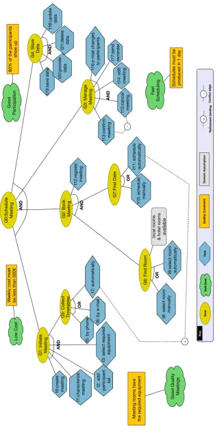
Goal Models. In this thesis we also use goal models for representing stakeholder requirements. A goal model captures both functional and non-functional requirements, referred as hard goals and soft goals respectively. Hard goals areAND/OR-refined until each goal is operationalized by tasks. Along with goals, domain assumptions represent preconditions that must hold for the system to operate properly.
Figure 2.1 captures the requirements of a Meeting-Scheduler system [LDM95] that is meant to facilitate the process of organizing meetings in a large institution. For the system to satisfy its top goal ScheduleMeeting, every time a meeting request arrives, must initiate a meeting by creating a new meeting event, collect the participant list, the meeting’s topic and the required equipment for the meeting. Next, the timetables are collected by each participant either by e-mail, by phone or automatically by the system. In order for the system though to collect the timetables the domain assumption that participants use the system calendar must hold. Then, a date and room must be selected either manually by the meeting organizer or automatically by the system. In addition, the system must allow the meeting organizer to confirm or cancel the occurrence of the meeting, send invitations to the participants and modify the date or the topic if needed. Finally the system must store all the date related to the meeting and make them accessible to the meeting organizer.
G0:Schedule
Meeting
A
ND
G1: Initiate Meeting
t0:cr eate meeting t2: add participant list A ND
t3: select r
equir ed equipment t1:characterize meeting G4: Stor e Data t19:save data t20:pr ovide data t21:delete data A ND t18:update data
G3: Manage Meeting
A
ND
t14: edit meeting
t15:cancel meeting
t13:confirm meeting
t16:e-mail changes
to participants t17:send reminder
G2: Book Meeting
A ND t12:r egister meeting Low Cost W
eekly cost must
be less than 500€
Good
Participation
80% of the participants
show up
Fast
Scheduling
Schedules must be pr
oduced in 1 day
Good Quality Meetings
Meeting r
ooms have
the r
equir
ed equipment
t11: schedule automatically
G7:Find Date
t10: schedule
manually
OR
G6: Find Room
OR
t8: select r
oom manually t9:select r oom automatically local r ooms
& hotel r
ooms
available
G5: Collect Timetables
t7: automatically
t6: by e-mail
t5: by phone
instance, Fast Scheduling may be operationalized by minimizing the time it takes to schedule meetings.
A goal model for a self-adaptive system captures the functional require-ments for the system-to-be. The system at runtime can switch among alternative refinements where this is possible, in order to guarantee the satisfaction of all root goals. However, choices among alternatives can be constrained. For instance, as Figure 2.1 shows, if the timetables are collected automatically then the meeting’s date must be selected automat-ically by the system as well. Such relationships are called goal constraints
[NSGM16a] and capture dependencies among goals.
2.1.3 Requirements monitoring
As explained in the previous Chapter, one of the fundamental components of an adaptation mechanism is monitoring. A system must be aware of its goals and the degree in which they are fulfilled at runtime [SBW+10]. Fickas and Feather in their work [FF95] explore the need of specifications with focus on monitoring requirements of systems that operate in ever-changing environments.
Figure 2.2: States assumed by requirements [SLRM11].
example, the goal CollectTimetables of the Meeting-Scheduler exemplar must be fulfilled every time a new request arrives and therefore, a new instance of this goal is created. Goal instances go through certain states as shown in Figure 2.2. When the goal instance is created its state is Undecided. Eventually as the system pursues to fulfil the goal, the instance will either have Succeeded or Failed. In case the goal is taking too long to be fulfilled, another potential state is Cancelled.
Low Cost
Weekly cost must be less than 500€
(AR1) SuccessRate(85%)
(a)
t11: schedule automatically G7:Find Date
t10: schedule manually
OR
(AR8)
ComparableSuccess (schedule manually, 10)
(AR5) NeverFail
(b)
Figure 2.3: Aggregate Awareness Requirements.
Awareness Requirements (AwReqs) are associated with goals, tasks, do-main assumptions and quality constraints. The monitoring mechanism, every time a new instance of a goal is created records every change in its state. This allows to measure the success of requirements over time. For example, the quality constraint of the soft goal Low Cost prescribes that the weekly cost of meetings must be less than 500e. In Figure 2.3a the
sched-ule manually. Such AwReqs that monitor the states of other requirements over the time are referred as aggregate AwReqs.
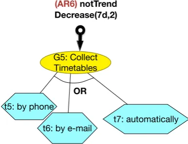
Trend AwReqs is yet another type of AwReq that compares success rates over a number of periods. For example, in Figure 2.4 AR6 prescribes that the success rate of the goal Collect Timetables should not decrease two weeks in a row. This type of AwReqs is used to identify how success/fail rates evolve over time.
(AR6) notTrend Decrease(7d,2)
G5: Collect Timetables
t7: automatically t6: by e-mail
t5: by phone OR
Figure 2.4: Trend Awareness Requirement.
A third type of AwReq are the Delta AwReqs. This type focuses on specifying acceptable thresholds for fulfilling the constrained goals. For in-stance, AR9 in Figure 2.5 specifies that when the meeting’s date is sched-uled manually, the task must be completed within one hour.
(AR9) StateDelta(Undecided,*,1h)
t10: schedule manually
Figure 2.5: Delta Awareness Requirement.
Language (OCL) [Rob07] and the values of their success rates are captured by variables named indicators. For example, indicator I1 = 85% means that the 85% of the times the quality constraint for the goal Low Cost is satisfied and therefore, AR1 succeeds. Listing 2.1 depicts the OCL con-straint for AR1 where Q CostLess500 is the class of the quality attribute of the Low Cost soft goal.
- - AwReq AR1: QC ‘Weekly cost must be lesss than 500e’ should have success
rate 85%.
c o n t e x t Q _ C o s t L e s s 5 0 0
def : all : Set = Q _ C o s t L e s s 5 0 0 . a l l n s t a n c e s ()
def : s u c c e s s : Set = all - > s e l e c t ( x | x . o c l I n S t a t e ( S u c c e e d e d ) ) inv AR1 : a l w a y s ( success - > s i z e () / all - > s i z e () >= 0 . 8 5 )
Listing 2.1: AR1 in OCL
2.1.4 Variability in goal models
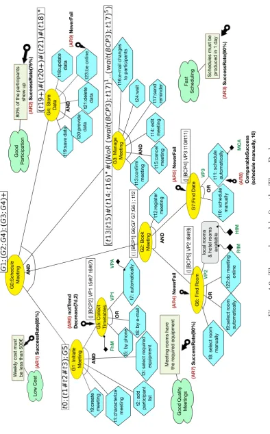
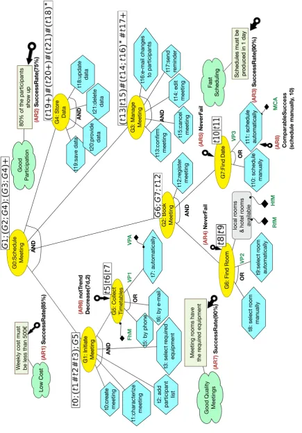
For an adaptive system it is useful to implement all alternatives that are captured as OR-refinements in the goal model because this allows multiple reconfigurations during adaptation. Hence, some (in our example, all) OR refinements can be marked as variation points (see labels VP1–VP3 in Figure 2.6). In this case, all tasks associated with each variation must be implemented and the system can switch from one configuration to another during adaptation [SLM11], as long as it adheres to its behaviour model
(discussed next).
Another source of variability along the requirements dimension consists of control variables. These represent the amount of resources and effort allocated for the system-to-be while it fulfils its requirements. For instance,
FhM representsfrom how many participants the system should collect time tables before goal G5 is considered satisfied (a percentage value). MCA
is another control variable that represents the maximum conflicts allowed
for the timeslot chosen for the meeting and participant time tables. RfM
are reserved for meetings, and finally VPA indicates whether the system has authorization to access personal time tables.
Control variables and variation points, hereafter requirement control pa-rameters (ReqCPs), can be adjusted at runtime by the adaptation mech-anism, to fix failing AwReqs. The qualitative relation between AwReqs
and parameters is captured through a systematic process called qualitative system identification1. During this process the domain expert captures the positive or negative influence that a parameter change can have on an
AwReq. More specifically, the differential relationship ∆(I2/M CA) < 0 means that by increasing MCA by one unit the success rate of AR2 will decrease. Similarly, ∆(I5/M CA) > 0 means that by increasing MCA the success rate of AR5 will increase. Differential relations are symmetric with respect to increases/decreases, meaning that if MCA is decreased the success rate of AR5 will also decrease.
2.1.5 Requirements Evolution
Requirements elicitation is not an easy task and stakeholders often change their minds during the development of the system-to-be or after the system is delivered. Moreover, setting thresholds for soft goals and constraints is not easy either, especially because some of these goals are conflicting and estimating an equilibrium is almost impossible until the system is deployed. In other cases, stakeholders have very high expectations from the system that cannot be always met due to external disturbances which are not captured during the design phase.
In order to cope with these challenges we use a new kind requirements, named Evolution Requirements (EvoReqs) [SLAM13]. This type of re-quirements specifies required changes to other rere-quirements when certain
1In the original work presented in [SLM11] the process is referred simply as system identification. To
G0:Schedule
Meeting
A
ND
G1: Initiate Meeting
t0:cr eate meeting t2: add participant list A ND
t3: select r
equir ed equipment t1:characterize meeting G4: Stor e Data t19:save data t20:pr ovide data t21:delete data A ND t18:update data
G3: Manage Meeting
A
ND
t14: edit meeting
t15:cancel meeting
t13:confirm meeting
t16:e-mail changes
to participants t17:send reminder
G2: Book Meeting
A ND t12:r egister meeting Low Cost W
eekly cost must
be less than 500€
(A R1 ) SuccessRate(85% ) Good Participation
80% of the participants
show up (A R2 ) SuccessRate(75% ) Fast Scheduling
Schedules must be pr
oduced in 1 day
(A
R3
)
SuccessRate(90%
)
Good Quality Meetings
Meeting r ooms have the r equir ed equipment (A R7 ) SuccessRate(90% ) (A R6 ) notT rend Decr ease(7d,2 ) (A R4 ) NeverFail (A R5 ) NeverFail MC A
t11: schedule automatically
G7:Find Date t10: schedule manually OR (A R8 )
ComparableSuccess (schedule manuall
y, 10
)
G6: Find Room
OR
t8: select r
oom manually t9:select r oom automatically HfM local r ooms
& hotel r
ooms
available RfM
G5: Collect Timetables
t7: automatically
t6: by e-mail
t5: by phone
conditions apply (e.g., the failure of an AwReq). For example, If require-ment R fails three times in a row, replace it with requirerequire-ment R0, where R is a weaker (i.e., easier to fulfil) requirement. Such requirements are use-ful to evolve unfeasible requirements that were initially elicited from the stakeholders.
EvoReqs are applied by operations that are triggered by preconditions specified by stakeholders and designers. The triggering events can be a re-quirement failure of a scheduled event. Furthermore, the changes applied can either be permanent or temporary. Table 2.1 presents EvoReqs oper-ations specified for the Meeting-Scheduler system. For example, when the system receives large amount of requests because a special event is taking place, or when the prices of the hotel rooms rise, the 85% threshold set by AR1 becomes infeasible. Therefore, when one of the aforementioned events takes place, the threshold is relaxed to 75% by the EvoReq opera-tion Relax(AR1,AR10 75). When the environment returns to its previous state, meaning that the meeting requests are reduced, or the prices are decreased the threshold can be restored to the values by the EvoReq oper-ation Strengthen(AR1,AR10 85). Other EvoReq operation might indicate that the system should wait for a certain amount of time before evaluating again the success of an AwReq as in the case of AR6 and AR7 or replace it permanently with another one such AR5.
2.1.6 Software Architecture Modelling
fulfil-Table 2.1: EvoReqs operations
AwReq EvoReq operation
AR1 1. Relax(AR1,AR1
0 75)
2. Strengthen(AR1,AR10 85)
AR2 Relax(AR2,AR20 90)
AR3 Relax(AR3,AR30 90)
AR4 1. wait(3 days)
2. Relax(AR4,AR40 75)
AR5 Replace(AR5,AR50 3)
AR6 wait(3 days)
AR7 wait(2 days)
ment is achieved.
More specifically, David Garlan in [Gar14] illustrates six aspects that software architecture contribute to software development. First, software architecture allows a better understanding of large and complex systems, since a high-level design is more comprehensible. Next, architecture design allows designers to reuse solutions to similar problems and facilitates the construction of the system-to-be. Moreover, when new components must be added or older ones are modified, the designers can reason about the impact on the system’s integrity.
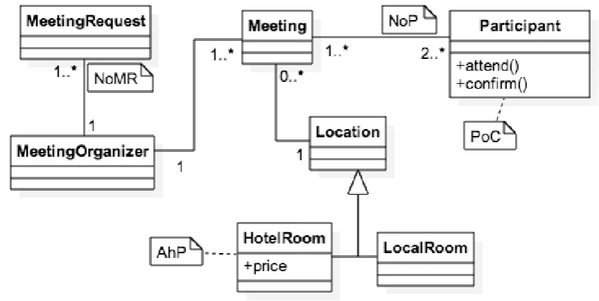
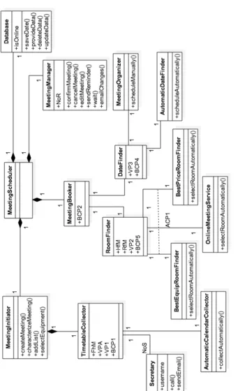
Figure 2.7: Architectural diagram for the Meeting-Scheduler
have been neglected by the software industry. Therefore, for our purposes, we use class diagrams to represent an architecture [ICG+04], where classes model components, while associations model connectors. Other types of re-lations between classes (e.g. composition) capture the structural rere-lations of the system. For example, the class diagram in Figure 2.7 shows the architecture of the meeting scheduler system, where the TimetableCollec-tor component is part of the MeetingInitiaTimetableCollec-tor component and can interact with one or more Secretary components.
2.1.7 Software Behaviour Modelling
Another aspect of software systems is their behaviour and by that we mean the sequence in which the components execute their assigned tasks. There is rich literature on languages that describe software behaviour, such as Petrinets [Mur89], Statecharts [Har87], and BPMN [Whi04]. In this work, we represent the behaviour of the system using flow expressions [PCM+14, DBHM13] as attachments to each goal (in Figure 2.6, goals G0–G7). These are extended regular expressions that describe the flow of system behaviour, with each atomic component of allowed sequences of fulfilment of sub-goals that lead to the fulfilment of a parent goal.
The operators ; (sequential), | (alternative), opt() (optional), * (zero or more), + (one or more), # (shuffle) allow us to specify sequences of system actions that constitute a valid behaviour. Shuffle specifies that its operands are to be fulfilled concurrently. For example, G0 # G1 means that goals G0 and G1 are to be fulfilled in parallel. Of course, each of these goals has its own flow expression to describe in what order its own subgoals and tasks are to be fulfilled/executed.
Behavioural models contribute to disambiguating certain refinements of the goal models. For instance in Figure 2.6, Manage Meeting is AND-refined to five tasks. From a design point of view, this means that all the five functionalities must be supported by the system-to-be. However, at runtime, it is not an acceptable behaviour to cancel and confirm the same meeting.
2.2
Dynamic System Modelling
quanti-tative models for software systems. However, in many cases, a sufficiently accurate analytical model, can be obtained through system identification techniques [Lju99], and can be used for control design. Letting u(t) ∈ Rm be the vector of m control parameter values at time t, andy(t) ∈ Rp be the vector of p indicators, their respective dynamic relation is described as:
yi(t) = p
X
j=1
ny X
k=1
αijkyj(t−k) + m
X
j=1
nu X
k=1
βijkuj(t−k) (2.1)
for all i = 1, . . . , p, and with αijk ∈ R, βijk ∈ R. The quantitative dy-namic model (2.1) relates the values of the indicator yi at time t with past values of all the indicators – accounting for possible mutual influences of the indicators – and with past values of control parameters. For ex-ample, I1, that measures the success rated of the Low Cost goal in the Meeting-Scheduler exemplar, might achieve a high value because of good management of hotel room assignments or because of the constant failure of I4, the success rate of Find Room. The reason is that if meetings fail to be scheduled, no rooms are reserved and consequently the cost of meetings remains low. Such implicit relationships among indicators can be cap-tured by model (2.1) to guide the adaptation process. Notice that if some of the mentioned variables are not influencing the value of the indicator
yi(t), then the corresponding parameters are simply zero. An equivalent and more compact representation of this relation is the discrete-time state-space dynamic model:
x(t+ 1) = Ax(t) + Bu(t)
y(t) =Cx(t),
(2.2)
the system, and it is not necessarily measurable. The values of the matrices (A, B, C) fully describe how the inputs dynamically affect the outputs of the system, and these matrices are the outcome of the System Identification process.
The analytical model of Equation (2.1) shows that the system’s output might be related to past outputs and control inputs. Indicators related to aggregate AwReqs [SLRM11] express success rates over time about the satisfaction of an associated goal and, therefore, their current values are naturally bound to their past values and to the values of AwReqs that produced them. These are dynamic systems in Control Theory. In case no relation with past behaviour of the indicators and of the control inputs is present, A is a matrix with all zero elements, and the system is just mapping inputs to outputs with the static relation:
y(t) =CBu(t−1).
Therefore, the model of Equation (2.2) accounts for both dynamic and static systems.
Equation (2.2) can be used to design a control system able to adjust the values of every control parameter, in order to make each indicator converge to the value prescribed by an AwReq threshold — under the assumption that the set of chosen control parameters is able to drive the system to the prescribed goals. In contrast to qualitative adaptation, such quanti-tative models allow one to handle conflicts with precision. For example, an increase of the control parameter M CA results in an increase of I5, the success rate of Find Date, as it becomes easier to find a commonly agreed timeslot for the meeting, but the participation might drop and con-sequently I2, the success rated of High Participation, is decreased. The analytical model can prevent the adaptation mechanism from decreasing
account priorities among indicators based on their business value (higher priority indicators should converge faster than less important ones), and preferences among control parameters (e.g. increasing Rf M is preferred to increasing Hf M) is a complex process. In chapters 7 and 8 we present a control-theoretic approach in order to efficiently implement this process and maintain an equilibrium among conflicting goals.
2.3
Related Work
In the past decade the literature in the area of self-adaptive systems has been enriched with multiple proposed frameworks, languages and tech-niques. In this section we present the state-of-the art of such approaches dividing them in four categories. First, we present approaches for software adaptation that use requirements, architectural and behavioural concep-tual models or combinations of them. Finally, we conclude this Section with approaches that apply control theoretic techniques.
2.3.1 Requirements-based Adaptation
A well-known Requirements-based approach is RELAX [WSB+10], which aims at capturing uncertainty declaratively with modal, temporal and or-dinal operators applied over SHALL statements (e.g., “the system SHALL ... AS CLOSE AS POSSIBLE to ...”). A recent extension of this work, AutoRELAX [FDC14], uses genetic algorithms in order to produce RE-LAXed goal models to change system requirements for avoiding failures caused by environmental uncertainty.
ex-actly equal to the desired ones. FLAGS also proposes an operationalization of its models in a service-oriented infrastructure.
The LoREM approach [GSB+08], also based on KAOS, uses an exten-sion of LTL that includes an Adapt operator and defines a systematic pro-cess for performing goal-oriented RE for adaptive systems. Later, Cheng et al. [CSBW09] integrated this approach with the RELAX language in order to explore environmental uncertainty using threat modelling.
In [ZSL14] the authors propose the use of a cost-function for optimizing the non-functional requirements of the target system, captured by goal models, while minimizing the number the penalties taken for violating Service Level Objectives. The available adaptations are ranked with the use of the Analytic Hierarchy Process (AHP) [Saa80] by the designers before the system’s deployment. Then, by applying a search-based method the adaptation which would optimize the cost-function is selected.
Another requirements-based and control theoretic approach is presented in [PCYZ10]. In this work the authors propose the use of a PID controller that finds a different configuration over a goal model that captures the system requirements. A SAT-solver is used to find the best configuration based on goal preferences. When soft-goals are not met, the controller tunes the values of the assigned preferences in order fors the SAT-solver to find a better configuration.
There are also a few RE-based approaches for the design of adaptive sys-tems based on i∗ [YGMM11] and Tropos [BPG+04]. Tropos4AS [MPP09] is a methodology for the design of agent-based adaptive systems founded on the Belief-Desire-Intention (BDI) model. As run-time infrastructure, Tropos4AS proposes the mapping of goal models to Jadex.2 The CARE method [QP10] also bases itself on Tropos, but focuses on service-based applications. Adaptive requirements are specified at design time and a
run-time infrastructure based on environment monitoring, service selec-tion and customizaselec-tion is provided. Dalpiaz et al. [DGM12] propose an architecture that adds self-reconfiguring capabilities to a system using a Monitor-Diagnose-Compensate (MDC) loop based on the system’s require-ments models in i∗. Different reconfiguration algorithms are proposed on top of this architecture.
2.3.2 Architecture-based Adaptation
In [OGT+99] Oreizy et al. propose one of the first reference frameworks for architecture-based adaptation. On the foundations of this approach there is an architectural model constructed using C2 [MTWJ96] which captures the properties and the component structure of the system. The purpose of the architectural model is twofold. First, it allows to maintain the integrity of the system as the system evolves by adding and removing components. Next, the proposed reference framework includes a planning mechanism that produces adaptation plans on the fly to cope with the environment’s uncertainty, The architecture model facilitates the planning process by giving an overview of the systems status and hence locating where changes are required.
failure. In the same research line, in [CGSP15] the authors propose the use of probabilistic model checking techniques to compose dynamically adap-tation strategies taking also into account latencies about when the impact of a change in a control parameter will appear to the system’s output.
Sykes et al. in their work [SHMK10] assign utility properties to all components of the system. Dependency graphs are used to capture com-ponent constraints and each comcom-ponent is annotated with utilities that indicate how it will improve or harm the non-functional requirements of the system. When one or more requirements fail the proposed adaptation mechanism finds a new component composition that maximizes the the overall utility and at the same time respects the architectural dependen-cies and constraints. Similar to this approach, the SASSY framework uses optimization as a decision-making mechanism to decide alternative service compositions for Service Oriented Architectures (SOA) [MGMS11]. In the same context Foster et al. propose an online reconfiguration process for SOA, that exploits prediction models in order to anticipate environmental changes such as workload peaks.
Another architecture-based approach is presented in [SBP+08]. In this work, the authors propose a resource provisioning system that allows the users to state their preferences about the quality of service of the system. For instance, the users have to choose if latency or accuracy is more im-portant for them and as well as they expected thresholds they expect the system to comply with. Therefore, the adaptation framework will perform trade-offs based on the user preferences producing adaptation plans that include resource provisioning and forecasting.
communica-tion protocol gossip which is used by the system’s components in order to inform each other about their status. When a requirement fails or a com-ponent is malfunctioning, the healthy comcom-ponents which are individually aware of the system’s architecture and goals, coordinate in order to deploy new components or assign tasks to existing ones in order for the system to recover.
2.3.3 Behaviour-based Adaptation
In [LYM07], Lapouchnian et al. describe how to derive high variability business process models that capture the system’s behaviour from goal models. The behaviour derivation process is carried out by annotating flow expressions to goal models as it is demonstrated in Section 2.1.7. Then, these expressions are converted to BPEL [Jur06] processes. Finally, using the contributions of the hard goals to the soft goals specified by the stakeholders and the system designers a configuration is decided. The contribution of this proposal is the construction of high variability business processes that can adapt to changes of stakeholder preferences.
Another behaviour-based approach is the CEVICHE framework [HSD10] which uses a Complex Event Processing engine to identify exception to the regular business process. These exceptions are handled with predefined adaptation that are encoded in a BPEL variation, namely SBPEL. This case-based adaptation mechanism allows to maintain a specific level of Quality of Service (QoS) without having to implement all the potential variations of the business process since the system can reconfigure dynam-ically.
select-ing values for the variation points of the workflow, based on the input of the adaptation process.
2.3.4 Combined Model-based Adaptation
Having as a starting point a goal model, Yu et al. [YLL+08] propose heuristics to derive other models such as feature models, statecharts and component-connector models. Their purpose is to express the same level of variability in different dimensions of the system.
The STREAM-A approach presented in [PLC+12] derives ACME ar-chitectural models from goal models using model transformations. The environment’s influence on the requirements is captured in terms of con-text. The main purpose of this work is to relate the requirements to compo-nents and place accordingly the actuators and the sensors of the adaptation mechanism.
In [SHMK08] goals and components are related with reactive plans. When a failure takes place or a goal is changing, the proposed adaptation mechanism generates a new plan of actions that needs to be carried out and the available components that are required are reconfigured to the current architecture. This approach demonstrates the advantages of architectural variability, by assigning goals to multiple components.
2.3.5 Control-based Adaptation
Most approaches that have been proposed have in common the adoption of the concept of feedback loop from Control Theory. As we mentioned earlier Control Theory has solved in multiple domains of other engineering disciples adaptation problems, where a quantitative goal and one or more control parameters are available. Recently, there has been some significant effort on introducing control engineering approaches in the development process of self-adaptive software systems [FMA+15]. Hereby, we present approaches that have applied formal control theoretic techniques in order to develop adaptive software systems.
One of the first proposals that builds a controller as an adaptation mechanism is presented in [PGH+01]. In this work the authors use an ana-lytical model to capture how the allowed number of remote procedure calls to an IBM Lotus Domino server affect its response time. Therefore, the analytical model captures the relationship of these two variables through time. Then this information is used in order to build an integral controller that can stabilize the response time to the given reference input. In addi-tion to this work, building various kinds for controlling computing systems [HDPT04] and resources in operating systems [LMPT13] are present in literature.
extended their approach in order to deal with MIMO systems [FHM15] where the MIMO control is obtained as an automated synthesis by com-posing SISO controllers in a hierarchical way.
Finally, in the domain of Cloud Computing variations of Model Pre-dictive Control (MPC), which we discuss in detail in chapter 7 have been applied extensively. In [GC15, KKH+09] the authors apply look-ahead con-trol to improve the energy consumption and the performance of the cloud. Similarly, in [GLPB14] MPC is applied to improve the replica placement mechanism and deal with multiple SLOs.
All these approaches offer significant improvements to their respective applications, although are highly customized to the specific problem they are solving. On the other hand, our approach is more generic and therefore easier for software engineers that have no expertise on Control Theory to use it. Moreover, in our work we integrate control design and requirements engineering in order to provide a guideline about to how to integrate MPC with the development of self-adaptive software.
2.4
Chapter Summary
EvoReqs that prescribe how other requirements should change over time. The last piece of our baseline describes how a system can be described using analytic models and how the latter are related to the system’s goals and variables.
Requirements and Architecture
Approaches: A Comparison
Computer Science is a science of abstraction -creating the right model for a problem and devising the appropriate mechanizable techniques to solve it.
A. Aho and J. Ullman
In Section 2.3 we presented various proposals, intended to guide develop-ers in the development of self-adaptive systems, some focus on architecture models that capture architectural variability and support reconfigurations in the system’s structure, propagating the effects to the actual system, in response to certain situations. Instead, other approaches, advocate the use of requirements models to capture variability and support adaptation.
This dichotomy has motivated us to investigate whether these two types of approaches can produce the same results, what are their respective ad-vantages and drawbacks, and study whether they are complementary, pro-viding answers to RQ1.
both frameworks to the same exemplar: the ZNN.com case study presented in [CGS09] for the Rainbow framework. Models of the system’s adaptation rules were produced for each framework and adaptation scenarios based on an implementation of ZNN.com were executed.
3.1
Selected Adaptation Approaches
In the previous chapter we overviewed several approaches that use various kinds of models in order to adapt when they fail to fulfil their mandate. In the literature the two most common models used for software adaptation capture either the requirements or the architecture of the target system. Therefore, we selected a representative framework for each category to analyze the characteristics of both kinds of models and their role in the adaptation process.
• Requirements-based (henceforth RE-based) approaches: extend
Requirements Engineering techniques in order to represent the re-quirements of adaptation and/or the inherent uncertainty of the en-vironment in which the system operates. These approaches may or may not include mechanisms for runtime reasoning and frameworks that operationalize the adaptation requirements, since they focus on capturing and analyzing the problem rather than implementing solu-tions.
• Architecture-based approaches: concentrate on helping designers
As we mentioned earlier, for our comparative study, we selected the Zan-shin and Rainbow to represent requirement and architecture-based adapta-tion frameworks respectively. These frameworks were chosen for a number of reasons. Firstly, they are good representatives of their respective schools of thought on building adaptive software systems. Secondly, they are fairly comprehensive and quite well documented in guiding the design of adap-tive systems. Thirdly, there was code readily available for running our experiments. We summarize both approaches next.
3.1.1 Rainbow
The Rainbow framework [GCH+04] is a prominent architecture-based ap-proach for the design of self-adaptive systems. According to the proposal, adaptation rules are used to monitor the operational conditions of the sys-tem and define actions to be taken if the conditions are unfavourable. For example, given a news website (which we will detail in Section 3.2), if mea-sured response times are too long, actions such as enlisting more servers or switching from multimedia to textual mode can be executed to try and improve response time.
The framework prescribes the use of the ACME architecture description language [GMW10], which extends the usual component-connector repre-sentation with the concept offamilies, allowing designers to define different architectural variants and styles [SG02]. This allows for the specialization of the framework to specific application domains, defining style-specific architectural operators and repair strategies [GCS03].
Figure 3.1, adopted from [Che08], shows the elements that compose the
Rainbow framework. Monitoring is done with a set of Probes deployed in the target system, which send observations to Gauges that interpret the probe measurements in terms of higher-level models. The Model Manager
Figure 3.1: The components of theRainbow framework [Che08].
consistent with the target system. Moreover, other components query the Model Manager for information about the current state of the model.
One of these components is the Architecture Evaluator, which detects changes in the status of the properties of the system’s architecture and en-vironment, validating such changes with respect to the constraints stated in the model. In case of a violation, it triggers the Adaptation Manager in order for it to select the most appropriate strategy, using Utility Theory (details in [Che08]) for the decision. Finally, the Strategy Executor coordi-nates the execution process, deciding the operators that should be applied through the Effectors at the System Layer.
Figure 3.2: An overview of the Zanshin approach [SS12].
what, when and how to adapt, thus automating the adaptation process. In Section 3.2 we will see some examples of Stitch applied to the exemplar chosen for our experiments, the news website ZNN.com [Che08].
3.1.2 Zanshin
Zanshin, is an RE-based framework for the design of adaptive systems that exploits concepts presented in the previous section such as AwReqs,
EvoReqs and feedback loops to design adaptive software systems [SS12]. The core idea of the approach is to make the elements of the feedback loops that provide adaptivity first class citizens in the requirements models. An overview of the approach is shown in Figure 3.2. In particular, Zanshin
uses AwReqs is its monitoring mechanism and differential relations as a basis of its adaptation.
loop. Its objective is to associate one or more adaptation s
![Figure 3.1: The components of the Rainbow framework [Che08].](https://thumb-us.123doks.com/thumbv2/123dok_us/533502.2053185/64.595.80.486.138.443/figure-components-rainbow-framework-che.webp)
![Figure 3.2: An overview of the Zanshin approach [SS12].](https://thumb-us.123doks.com/thumbv2/123dok_us/533502.2053185/65.595.102.540.152.399/figure-overview-zanshin-approach-ss.webp)