http://www.sciencepublishinggroup.com/j/ijamtp doi: 10.11648/j.ijamtp.20180402.15
ISSN: 2575-5919 (Print); ISSN: 2575-5927 (Online)
The Solution of the Wave Equation in the Class of Complex
Numbers by Introducing Hyperbolic Coordinates
Khoroshavtsev Y. E.
Faculty of Automatic Control Systems, State University of Civil Aviation, St. Petersburg, Russia
Email address:
To cite this article:
Khoroshavtsev Y. E. The Solution of the Wave Equation in the Class of Complex Numbers by Introducing Hyperbolic Coordinates. International Journal of Applied Mathematics and Theoretical Physics. Vol. 4, No. 2, 2018, pp. 61-66. doi: 10.11648/j.ijamtp.20180402.15 Received: May 13, 2018; Accepted: August 19, 2018; Published: September 17, 2018
Abstract:
The finding of the solution of the wave equation, formulated as the Cauchy problem, does not exhaust all possibilities of the theory. The attempt to examine that one by admitting that the time is an imaginary value is made. So the new curvilinear coordinates, named hyperbolic, are introduced in consideration. They allow for hyperbolic equations to extend a field of searching of solutions to the complex plan and give the possibility to apply powerful Fourier’s method. Due to that, the wave equation takes a form of Laplace’s one in polar coordinates. However, the boundary condition differs from well known Dirichlet problem that in this case looses the sence. The new condition is admitted and it is physically formulated as the description of wave from various inertial systems of coordinates. So the result is obtaining proceeding either of the momentum picture of a wave, made from the moving system of coordinates, or on the oscillogram, developed in time The analytic solution that differs from Poisson integral is deduced and gives the formulas of relativistic addition of velocities for points of wave, observing from different inertial systems. That integral was also formally yielded by using the conform translation. Additionally, in the frequencies field those formulas describe the relativistic Doppler’s effect and the red shift in the wave spectrum. For oscillatory boundary condition the solution of the obtained integral gives a description of the shock waves. The fact, that some formulas of Relativity may be deduced by new way, gives the possibility to explain the relativistic theory proceeding from supposition of waving nature of quantum objects.Keywords:
Wave, Equation, Fourier Transformation, Boundary Condition1. Introduction
The wave equation has a key matter to understand the laws of the nature. Maxwell one with Lorentz calibration can be led to it [2]. These equations are Lorentz invariant and give the theoretical argument for the creation of the Relativity [2, 13] that stresses there importance.
There are a lot of works dedicated to the solutions of the wave equation. They can be represented as a non-homogeneous or non-linear ones in different dimensions with appropriated results [11, 12]. Non-stationary equation with blowup is studied in [15]. The methods of solutions differ also, so in [16] the solving is based on the mathematical symmetry of the equation, digital methods are applied in [11, 14].
However, nearly all solutions lay in the class of real numbers that diminishes the field of a search. On the other hand, it is known that in electromagnetic theory or in the
quantum mechanics the complex solutions are largely applied. So it is interesting to examine the wave equation in the class of complex values. In order to achieve that it is necessary to look at the description of fundamental physical expressions. Such Schrödinger equation or Minkowski metric suppose that the time is an imagine value. In the further investigation that meaning will lead to the definition of the hyperbolic coordinates.
2. New Solution of the Wave Equation
2.1. Hyperbolic Equations in Hyperbolic Coordinates
Let there is a simplest hyperbolic equation
1 0
u u
x c t ∂ + ∂ =
∂ ∂ . (1)
It is known, that any smooth and differentiable function u
(ct-x) satisfies it [1, 3, 5].
Let's pass to new curvilinear coordinates r and φ, which will be named hyperbolic
2 2 2 , 0 ,
arth , 1 .
r c t x r
x
i i
ct
φ
= − ≥
= = − (2)
The physical sense of new variables will be done later. Changing independent variables x and t on r andφ, yields the function u (r, φ) [6].
Into new coordinates (1) can be rewritten as
0 .
u u
r i
r φ
∂ + ∂ =
∂ ∂ (3)
Though apparently the equation became complicated, the powerful Fourier method of separation of variables can be applied. So the solution of (3) is determined as
)
(
( , ) ( ) ( ) ,
u r φ =u L r Φ φ (4)
where u, L, Φ, - differentiable functions. Substitution (4) in (3) gives
( ) ( ) ( ) ( ) .
rΦφ L r′ = − Φi ′φ L r
That is the equation with separable variables
( ) ( )
,
( ) ( )
L r
r i
L r
φ λ
φ ′ = − Φ′ =
Φ
where λ ≠ 0 - a real number. From that two expressions issue
( ) ( ) 0 ,
( ) ( ) 0 ,
r L r L r i
λ
φ λ φ
′ − =
′
Φ + Φ =
with solutions
( ) ,
( ) ei .
L r rλ
λφ
φ =
Φ =
According (4) the required function is
( , ) ( i )
u r φ =u r eλ λφ (5)
with the parameter λ (proper number).
Admitting in (5) λ = 1, and returning to the ordinary x and t
variables, the well known function u (x, t) = u (ct – x) is obtained.
2.2. Wave Equation in Hyperbolic Coordinates
Let there is a homogeneous wave equation [3, 4]
2 2
2 2 2
1
0 .
u u
c t x
∂ −∂ =
∂ ∂ (6)
After introduction of the new coordinates r and φ according (2) in (6) and some rearrangements, the wave equation about required function u (r, φ) can be rewritten as
2 2
2 2 2
1 1
0 .
u u u
r r
r r φ
∂ + ∂ + ∂ =
∂
∂ ∂ (7)
It coincides with Laplace’s equation in polar coordinates. It seems that the well known solutions of Laplace’s equation can be borrowed if only the boundary conditions conserve a physical interpretation. However, there are difficulties in this way, which overcoming bear a supplementary investigation.
Certainly, it is not casually that the wave equation takes the form of Laplace’s one because of the fundamental link between trigonometric and hyperbolic functions in the domain of complex numbers.
First of all, to solve (7) it is necessary to formulate a boundary condition. In view of analogy with Laplace’s equation, it seems to be natural to admit external Dirichlet’s problem in which the boundary condition is set on a circle of radius r. However as against it, the physical sense is the other:
0 ( ) .
uφ φ= =f r (8)
It sets a shape of wave, which is observed from the inertial system of coordinates moving with speed v0=x t0 0 with respect to the laboratory one, so that φ =0 iarthv0 c.
Conditions of a problem are those. In the laboratory system of coordinates the source of oscillations which creates a wave is stiff. The moving observer in each j - time turns out in a point x0j=v t0 0j and registers amplitude of a wave fj. The
function
(
)
0
2 2
0 0
( ) 1
u φ = f r = f ct −v c sets a boundary
condition of a problem. The index 0 at x and t means that is not a concrete value, but the multitude of them, on which f (r)is defined.
Physically, the solution of equation must be obtained proceeding either of the momentum picture of a wave, made from the moving system of coordinates, or on the oscillogram, developed in time, of the oscillation of a point, moving with the velocity v0.
It depends on how to write the coordinate r (ct ≥ r):
2 2
2 2 2 0
2 2
0
1 1 v ,
c
r c t x x ct
v c
= − = − = −
The tasks with moving boundary are known in the theory of differential equations [7, 8], but they were solved on the basis of Dirichlet’s problem and differs from (8).
If φ0=0, i.e. v0=0 , that means that the observation is conducted from the Laboratory system of coordinates and the oscillations are described by f ct( 0).
It is possible to give to coordinate r such a physical sense. Admitting c=ω k, where ω - frequency of oscillation, and k - wave number, r can be written
(
)(
)
1
.
r t kx t kx
k ω ω
= + − (9)
i.e. r is equal to average geometrical phases of direct and return waves in scale k.
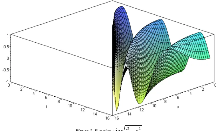
The shape of the wave with that phase differs from ordinary symmetric Sine wave (Figure1) that complicates the problem.
Figure 1. Function sin t2−x2 .
The required solution of the equation (7) might be obtained by means of Fourier’s method of separation of variables [6]
( ) ( ) .
u=Φφ L r (10)
Substituting this expression in (7) leads to
2
2
( ) ( ) ( )
, 0.
( ) ( )
r L r rL r
L r
φ λ λ
φ
′′ ′′ ′
Φ = − + = ≥
Φ (11)
Necessity of a positive sign before λ will be evident further: it follows from the requirement of periodicity of the solution on r.
The condition (11) breaks up to two equations:
2
( )φ λ ( )φ 0 ,
′′
Φ − Φ = (12)
2 ( ) ( ) 2 ( ) 0 .
r L r′′ +r L r′ +λ L r = (13)
Solving (12) it is obtained
. P eλφ Q e−λφ
Φ = + (14)
The solution of the equation (13) is searched as function
m
L r= . After its substitution in (13), m= ±iλ and
ln ,
i i r
L r= ±λ =e±λ
cos ( ln ) sin ( ln ) .
L A= λ r +B λ r (15)
By substituting (14) and (15) in (10) a particular solution becomes
[
cos ( ln ) sin ( ln )]
(
)
.uλ= A λ r +B λ r P eλφ +Q e−λφ
Arbitrarily it is admitted P=0, being confined with φ ≥0, where the sign before φ determines a sense of motion with respect to the motionless system of coordinates. Then
cos ( ln ) sin ( ln ) .
uλ=Aλ
λ
r +Bλλ
r e −λφHere A, B, P, Q, Aλ = AQ B, λ =BQ - constants of integration.
As λ - the continuous value, the general solution will be as follows
0
cos ( ln ) sin ( ln )
u e λφ Aλ λ r Bλ λ r dλ
∞ −
=
∫
+ (16)From the boundary condition (8) it leads to
0
0
( ) cos ( ln ) sin ( ln ) .
f r e λφ Aλ λ r Bλ λ r dλ
∞ −
Let's pass to a new variable α=lnr and, using the identity exp (ln )
r= r , rewrite a boundary condition f (r) as function
(ln ) ( )
fα r ≡ f α . It is obvious that −∞ < < ∞α . It is assumed that the function f (α) can be expressed by Fourier’s integral. Then
0
( ) cos ( ) ,
e
A f d
λφ
λ π α λα α
∞
−∞
=
∫
0
( ) sin ( ) .
e
B f d
λφ
λ π α λα α
∞
−∞
=
∫
By substituting these AλandBλ in (16) and following the
usual transformations, the required u can be written as
[
]
0 ( )
0 1
( ) cos ( ln ) .
u e λ φ φ f α λ α r dα dλ
π
∞ ∞
− − −∞
= −
∫
∫
Changing the order of integration gives
[
]
0 ( )
0 1
( ) cos ( ln .
u f α e λ φ φ λ α r dλ dα
π
∞ ∞
− − −∞
= −
∫
∫
(17)Integral in parentheses is tabular, its value is equal
0
( ) 0 0
2 2 2 2
0 0 0
( ) cos ( ln ) ( ln ) sin ( ln )
.
( ) ( ln ) ( ) ( ln )
r r r
e
r r
λ φ φ φ φ λ α α λ α φ φ
φ φ α φ φ α
∞
− − − − + − − = −
− + − − + − (18)
Substitution (18) in (17) leads finally to
0
2 2
0 ( )
( , ) .
( ) ( ln )
f d
u r
r
φ φ α α
φ
π φ φ α
∞
−∞
− =
− + −
∫
(19)The found integral gives the required solution of the wave equation in hyperbolic coordinates.
Let's examine its consequences. First of all it is interesting to investigate a simplest case r=1, i.e.exp (ln1)=1 or f (α)=1. Physically it means a constant phase of a wave. It is obvious that all points of a wave having the identical phase should have identical amplitude (the equation (6) does not describe a dispersion of energy). Really, the substitution the value f (α)=1 in (19) yields the tabular integral
0
0 0
1 ln 1
arctg 1
2 2
r
u φ φ α π π
π φ φ φ φ π
∞
−∞
− −
= = − − =
− −
A particular interest represents an oscillatory boundary condition. Let ln
( ) ein r , 0
f r = n> . Then f( )α =einα, and
ln ( ln )
ln
0 0
2 2 2 2 2 2
0 0 0
cos ( ln ) sin ( ln )
.
( ) ( ln ) ( ) ( ln ) ( ) ( ln )
in r in r
in r
e e n r d n r d
u d e i
r r r
α
φ φ α φ φ α α α α
π φ φ α π φ φ α φ φ α
∞ − ∞ ∞
−∞ −∞ −∞
− − − −
= = +
− + − − + − − + −
∫
∫
∫
The second integral by virtue of oddness of sub integral function equals zero, and the first one is tabular. The result is
0
( ) ln .
n in r
u e= φ φ− e (20)
For f( )α =exp (−inα) by analogy the similar function is
0
( ) ln .
n in r
u e= φ φ− e− (21)
Laplace’s equation is linear, therefore the superposition of solutions (20) and (21) results to
( ) cos
2
in in
e e
f n
α α
α = + − = α
0
( )
and u e= nφ φ− cos ( ln ).n r (22)
If φ=φ0 (22) satisfies to a boundary condition. It satisfies
also to the wave equation. That can be easily demonstrated by direct substitution (22) in (7).
The expression (22) has a singularity r =0, where lnr→ ∞. That takes place when x/t=c. When r→0 the function cos (lnr) describes the oscillations with increasing frequencies and in the limit the spectrum of the wave becomes like δ – Dirac function. That means, that the most part of energy is concentrated in the point, moving with constant speed v = c. That occurs in the shock waves.
relative speed, because the multitude of mutual - independent values x and t sets the choice of coordinates to describe the wave. But in case x/t=const (only) for all pairs of x, t, this ratio could be considered as a speed of the point in a space, in which the amplitude of a wave is registered. According to the definition of φ, this speed can be found by taking the modulus of the right side in (2). Then obviously,
th .
v x t c= = φ (23)
If boundary conditions are defined as in this case, in moving with a velocity v0 system of coordinates, and the wave is observed from the motionless system in a point which itself moves with velocity v with respect to a motionless system, then to find the relative speed of this point (from moving system), (23) takes the view
0 0
0
th th arth x arth x
v c c
ct ct
φ φ
′ = − = − =
0
0 0
0 0
2 0
. 1
1
x x
ct ct v v
c
x x v v
c ct ct
−
−
= =
− −
(24)
If c – a velocity of light, this is the formula of relativistic addition of speeds which they usually write down as
0 2 0
. 1
v v
v
v v c
′ + =
+ (25)
Here the ratio x0/t0 gives the same (boundary) value v0 to any pair from multitude {x0, t0}. Certainly, the concept of speed of a wave points is not universal and at arbitrary choice of x and t loses sense.
Let's return to initial variables. Assuming for simplicity
c2t2- x2>0 and using relationship
1 1
arth ln ,
2 1
z z
z + =
−
the formula (22) can be represented in a kind
(
2 2 2)
0 0
n
exp ln ln cos ln c .
2 2
c v
n ct x
u i t x
c v ct x
+ +
= − −
− −
(26)
If the boundary condition is given in motionless system of coordinates, then φ0=0, i.e. v0=0. For x/t=v=const, the formula (26) might be rewritten in more simple form:
1
2 ln
1
2
cos ln 1 , 0.
v c i
v c c
u e x v
v
−
+
= − ≠
(27)
From (27) it obviously follows that with distance from a source (with growth x) the wave is lengthened due to logarithmic smoothing. For light waves it should result to the red frequency shift in a spectrum.
In usual coordinates the formula (20) has the most compact view:
(
)
0 0 1
exp ln , 1.
1
v c
u i ct x n
v c
+
= − =
−
If in a boundary condition instead of r to put a dimensionless value kr, then the formula (26) appears in the more habitual form
2 2 2 2 0
0 1
exp ln cos ln .
1
v c t kx
u i t k x
v c t kx
ω ω
ω
+ −
= −
− +
(28)
The first radical in an exponent coincides with the expression of relativistic Doppler effect, that in general corresponds to earlier considered interpretation of a difference φ0-φ: for dot objects it yields a relativistic rule of addition of speeds; in frequency field - relativistic Doppler effect.
The solution (28) describes any (not only electromagnetic) waves, so relativistic formulas (25) - (28.) can be spread to them as well. Whether that is true or a mathematical trick can be proved only by an experiment. The term "relativistic" is certainly conditional because generally c is the phase’s velocity of diffusion of various waves (for example, acoustic). By decaying ln
(
ω2 2t −k x2 2)
=ln(
ωt−kx)
+ln(
ωt+kx)
, the solution (28) leads to both direct and return waves.The functions (26) - (28) describe the wave process in
motionless system of coordinates if the boundary condition is given in moving one with speed v0.
The obtained solutions can be applied to three-dimensional space. In this case, instead of x it is needed to put
2 2 2
x +y +z .
It is necessary to stress that the obtained formulas are true only in case of inertial systems. In general case it will be other solutions according to the new boundary conditions.
2.3. The Solution of the Wave Equation with Using the Conform Translation
{
r (0, ); φ φ( , )0}
,Ω = ∈ ∞ ∈ ∞
with polar coordinates r, φ.
Reflection of this field on the Cartesian semi plane y >0 in the domain of complex numbers with help of function
0 ln
z= ω φ−i , where ω=rexp ( )iφ , allows to use the general solution given by Dirichlet’s formula [9]
2 2
( )
( , ) .
( )
y f
u x y d
x y
α α
π α
∞
−∞
=
− +
∫
Here the components of z=x+iy are defined as x = ln r and
y=φ-φ0.
3. Result
The curvilinear coordinates named hyperbolic are introduced in consideration and the new solution of the wave equation in form of integral (19) is obtained. The examination of its particular consequences shows the link with the formulas of Relativity, namely, with the rule of relativistic addition of velocities and the formula of relativistic Doppler’s effect.
The using of the hyperbolic coordinates in hyperbolic equations gives the possibility to apply powerful Fourier’s method to obtain their new solutions.
The analysis of the wave equation with new coordinates can mathematically explain the nature of the shock waves, earlier not described.
4. Discussion
The fact, that some formulas of Relativity may be deduced by new way, gives the possibility to explain the relativistic theory proceeding from supposition of waving nature of quantum objects [10]. That concerns the fundamental basis of the contemporaneous physics and should be checked by the experiment, for example with the acoustic waves at the velocities approximately equal to sound. At first sight, the crazy idea can occur brainwave.
5. Conclusion
The extension of application of complex numbers to the solutions of physical equations leads, at first, to the new mathematical results, and at second, shows new properties of physical objects so that the time in many fundamental cases should be described in the form of imaginary value as in our solving.
References
[1] Godunov S. K. Equations of mathematical physics. Moscow, Science Publ., 1971, 416p. (In Russian).
[2] Richard P. Feynman, Robert B. Leighton, Matthew Sands. Feynman lectures on physics. Volume 1. London. 1963, p.196. [3] Morse P. M. Feshbach H. Methods of theoretical physics. Part
1. New York. McGraw-Hill, 1953.
[4] Tikhonov A. N., Samarskii A. A. Equations of mathematical physics. Moscow, Pergamon, 1963. (Translated from Russian). [5] Sobolev S. L. Partial differential equations of mathematical
physics. Pergamon. 1964. (Translated from Russian).
[6] Yu. E. Khoroshavtsev. Hyperbolic equations in hyperbolic coordinates. Bulletin of Civil Engineers. ISSN 1999-5571. St. Petersburg. April, 2014/2 (43), pp. 152-157. (In Russian). [7] N. Gonzalez. An example of pure stability for the wave
equation with moving boundary. Journal of mathematical analysis and applications. ISSN 0022-247x. vol. 228, Issue 1, December 1998, pp. 51-59.
[8] N. Balazs. On solution of the wave equation with moving boundaries. Journal of mathematical analysis and applications. ISSN 0022-247x. Vol. 3, 1961, pp. 472-484.
[9] Smirnoff V. I. Superior mathematics course. vol. 2. Moscow, Science, Publ., 1974, 656p. (In Russian).
[10] Yu. E. Khoroshavtsev. The wave interpretation of equations of relativistic dynamics. University Press. St. Petersburg. Mathematical Modeling, Digital Methods and Complexes of Programs. Vol. 10, 2004, pp. 164 – 172. (In Russian).
[11] B. Forneberg, G. B. Whitham. A numerical and theoretical study of certain nonlinear wave phenomena. Proc. R. Soc. Lond. 1978, pp 373-403.
[12] Dongbing Zha. Some remarks on quasilinear wave equation in 3-D. Mathematical methods in the applied sciences. Vol. 39, Issue 15, 2016, pp. 4484-4495.
[13] Ricardo Heras. Lorentz transformations and the wave equation. European journal of physics. Vol. 37, №2, 2016.
[14] G. M. Muslu, H. Borluk. Numerical solution for a general class nonlocal nonlinear wave equations arising in elasticity. ZAMM. Journal of applied mathematics and mechanics. Vol. 97, Issue 12, 2017, pp. 1600-1610.
[15] A. Y. Burtscher, R. Donninger. Hyperboloidal evolution and global dynamics for the focusing cubic wave equation. Communications in mathematical physics. Vol. 353, Issue 2, 2017, pp. 549-596.