ISSN: 2008-6822 (electronic)
http://dx.doi.org/10.22075/ijnaa.2017.1653.1436
A spline collocation method for integrating a class
of chemical reactor equations
Abdelmajid El hajajia,∗, Nadia Barjeb, Abdelhafid Serghinic, Khalid Hilalb, El Bekkaye Mermrid
aLERSEM Laboratory, ENCGJ, University of Choua¨ıb Doukkali, El jadida, Morocco bLMC Laboratory, FST, University of Sultan Moulay Slimane, Beni-Mellal, Morocco cMATSI Laboratory, ESTO, University Mohammed Premier, Oujda, Morocco
dDepartment of Mathematics and Computer Science, FS, University Mohammed Premier, Oujda, Morocco
(Communicated by S. Abbasbandy)
Abstract
In this paper, we develop a quadratic spline collocation method for integrating the nonlinear partial differential equations PDEs of a plug flow reactor model. The method is proposed in order to be used for the operation of control design and/or numerical simulations. We first present the Crank-Nicolson method to temporally discretize the state variable. Then, we develop and analyze the proposed spline collocation method for the spatial discretization. The design of the collocation method is interpreted as one order error convergent. This scheme is applied on some test examples, the numerical results illustrate the efficiency of the method and confirm the theoretical behavior of the rates of convergence.
Keywords: Partial differential equations; Distributed parameter systems; Plus flow reactors; Perturbed systems; Spline collocation method.
2010 MSC: Primary 58J10; Secondary 65D07.
1. Introduction and preliminaries
The plug flow reactor models are nowadays a necessity in chemical engineering and different catalytic processes with special needs have been lead to a wide variety of this class of tubular reactor models, since it reveal more informations about the reactor performance, and they can also be used for simulating steady-state and control operations (see eg., [12], [17]).
∗Corresponding author
Email addresses: [email protected](Abdelmajid El hajaji),[email protected](Nadia Barje),
[email protected](Abdelhafid Serghini),[email protected](Khalid Hilal),[email protected](El Bekkaye Mermri)
Usually, a dynamic tubular reactor model consists of PDEs and the practical method to integrate is to reduce them into a set of ordinary differential equations ODEs by spatial discretization, and to use well-known algorithms to solve the time-dependent model. This kind of systems are called distributed parameter systems DPSs and can be found in process control described by PDEs, e.g., robotics, bio-reactors, flexible structures, and vibrations (see e.g.,[1], [14]). These methods and algorithms are well described in several chemical engineering textbooks, (for example in [18, 7, 15]). Various numerical techniques have been developed and compared for solving the ODEs (see [3, 9]). Besides of the lack of knowledge of the connection between the original distributed parameter (infinite dimensional) model and its (finite dimensional) discretised version, the approximation methods may require extensive computation studies in order to try to capture the dynamic behavior of the DPS. For instance, the number of ODEs required in the finite differences method to obtain satisfactory model approximation many becomes excessively high (see [3]). Even when the methods of characteristics is able to provide an exact representation of the original model (see [9]) this attempt requires also a high number of collocation points which is difficult to implement in practical control and monitoring applications. The main objective of this study is to develop a user friendly, economical method which can work for solving a perturbed first-order hyperbolic PDEs model by using a quadratic splines collocation method.
Let us consider a chemical or a biological process taking place in a plug flow reactor whose mathematical model is given by
∂V
∂t (z, t) = −ϑ ∂V
∂z(z, t) +Kf(V(z, t)) +CV(z, t) +u(t), (z, t)∈Ω,
V(z,0) = α(z), z ∈Ωz,
V(0, t) = β(t), t∈Ωt,
(1.1)
In the above equations, V(z, t)∈RH is the state vector, f(V)∈
RS is the nonlinearities vector and Lλ-Lipschitz (Lλ ≥ 0), K ∈ RH×S denotes a matrix of known coefficients (e.g. stoichiometric or
yield coefficients), C ∈ RH×H is the state matrix whose elements are known, u(t) ∈
RH is a vector
gathering the process inputs (e.g. mass and/or energy feeding rate vector) and/or other time-varying functions (e.g. gaseous outflow rate). Besides, trepresents the time variable whereas z (z ∈[0, L]) is the axial position,Lis the reactor length,ϑis considered as a positive and known constant describing the velocity of the inlet stream,β(t) is a column vector which is a sufficiently smooth function of time and α(z) ∈ H[(0, L),RH] where HH[(0, L,
RH) being the infinite dimensional Hilbert Space of H
-dimensional-like vector functions defined on the interval [0, L]. The problem (1.1) can be formulated as the following problem
∂V ∂t +P
∂V
∂z −CV = I(V(z, t)), (z, t)∈Ω, V(z,0) = α(z), z ∈Ωz,
V(0, t) = β(t), t∈Ωt,
(1.2)
where
P = (diag(υ.Ij,j))j=1,...,H,
I(V) = Kf(V) +u(t)∈RH,
with Ci,j ≤eγ <0 on Ω and f,u, α, β are sufficiently smooth functions.
Here we assume that the problem satisfies sufficient regularity and compatibility conditions which guarantee that the problem has a unique solutionu∈C(Ω)T
C2,1(Ω) satisfying (see, [10, 8, 11]):
∂i+jV(x, t) ∂xi∂tj
where k is a constant in RH.
In the present work, we present a numerical method for solving the general dynamical model for a class of plug flow reactors. The method is based on Crank-Nicolson scheme to discretize the temporal variable and a quadratic spline collocation method for the spatial discretization. The scheme is one-order convergent with respect to the spatial variable.
The organization of the paper is as follows. In Section 2, we discuss time semi-discretization. Section 3 is devoted to the spline collocation method for solving the general dynamical model for a class of plug flow reactors using a quadratic spline collocation method. Next, the error bound of the spline solution is analyzed. In order to validate the theoretical results presented in this paper, we present numerical tests on two known examples in Section 4. Finally, a conclusion is given in Section 5.
2. Time discretization and description of the Crank-Nicolson scheme
Discretize the time variable by setting tm = m∆t for m = 0,1, ..., M, in which ∆t = T
M and then define
Vm(z) = V(z, tm), m= 0,1, ..., M.
Now by applying the Crank-Nicolson scheme on (1.2), we arrive at the following equation
Vm+1−Vm
∆t −
1 2L(V
m+1+Vm) = 1 2 I(V
m+1) +I(Vm) .
One way is to replaceVm+1 with Vm in the nonlinear terms. This leads to the following modified system:
Vm+1−∆t
2 LV
m+1 = ∆t
2 LV
m+Vm+ ∆tI(Vm). (2.1)
Form = 0,1, ..., M. The value of V at time levelm will be of the form:
P∂V m+1
∂z +RV m+1
= J(Vm), ∀z ∈[0, L],
V0(z) = α(z), ∀z ∈[0, L],
Vm+1(0) = βm+1, 0≤m < M.
(2.2)
where, for anym ≥0 and for anyz ∈[0, L], we have
R =
2
∆tI −C
,
J(Vm) = LVm+ 2 ∆tV
m
+ 2I(Vm),
L = −P ∂
∂z +CI,
Vm+1 is solution of (2.2), at the (m+ 1) th-time level.
The following theorem proves the order of convergence of the solution Vm toV(z, t).
Theorem 2.1. problem (2.2) is second order convergent, i.e.
Proof . We introduce the notation em =V(z, tm)−Vm the error at step m and
kemkH = sup z∈[0,L]
max
1≤i≤H|e i m(z)|.
By Taylor series expansion of V, we have
V(z, tm+1) = V(z, tm+12) +
∆t 2
∂V
∂t(z, tm+12) +
(∆t)2 8
∂2V
∂t2 (z, tm+12) +O((∆t) 3).I
H,
V(z, tm) = V(z, tm+12)−
∆t 2
∂V
∂t(z, tm+12) +
(∆t)2
8 ∂2V
∂t2 (z, tm+12) +O((∆t) 3).I
H.
By using these expansions, we get
V(z, tm+1)−V(z, tm)
∆t =
∂V
∂t(z, tm+12) +O((∆t)
2
).IH, (2.3)
and by Taylor series expansion of ∂V
∂t, we have ∂V
∂t (z, tm+1) = ∂V
∂t(z, tm+12) +
∆t 2
∂2V
∂t2 (z, tm+12) +
(∆t)2
8 ∂3V
∂t3 (z, tm+12) +O((∆t)
3).I
H,
∂V
∂t (z, tm) = ∂V
∂t(z, tm+12)−
∆t 2
∂2V
∂t2 (z, tm+12) +
(∆t)2
8 ∂3V
∂t3 (z, tm+12) +O((∆t)
3
).IH.
By using these expansions, and
∂3V
∂t3
≤c.IH on Ω (see relation (1.3)), we have
1 2
∂
∂t[V(z, tm+1) +V(z, tm)] = ∂
∂tV(z, tm+12) +O((∆t)
2
).IH.
This implies
∂V
∂t (z, tm+12) =
1 2
∂
∂t[V(z, tm+1) +V(z, tm)] +O((∆t)
2).I
H
= 1
2[LV(z, tm+1) +I(V(z, tm+1)) +LV(z, tm) +I(V(z, tm))] +O((∆t)
2).I
H.
By using this relation in (2.3) we get
(1− ∆t
2 L)V(z, tm+1) = (1 + ∆t
2 L)V(z, tm) + ∆t
2 [I(V(z, tm+1)) +I(V(z, tm))] +O((∆t)
3
).IH,
by (2.1). Then, we obtain
(1− ∆t
2 L)em+1 = (1 + ∆t
2 L)em+ ∆t
2 [I(em+1) +I(em)] +O((∆t)
3).I
H.
We may bound the termO((∆t)3) by c(∆t)3 for some c >0,and this upper bound is valid uniformly
throughout [0, T]. Therefore, it follows from the triangle inequality that
(I− ∆t
2 L)em+1 H ≤
(I+ ∆t 2 L)em
H
+∆t
2 (kI(em)kH +kI(em+1)kH) +c(∆t)
3
It follows from the Lipschitz condition we have
k(I −∆t
2 L)em+1kH ≤ k(I+ ∆t
2 L)emkH + ∆t
2 (kI(em)kH +kI(em+1)kH) +c(∆t)
3,
≤ k(I+ ∆t
2 L)kHkemkH + ∆t
2 kKkHkfkH(kemkH +kem+1kH) +c(∆t)
3
.
Clearly, the operator
IH ± ∆t
2 L
satisfies a maximum principle (see, [4, 5]) and consequently
IH ± ∆t 2 L −1 H ≤ 1
1 + ∆t 2 eγ
.
Since we are ultimately interested in letting ∆t → 0, there is no harm in assuming that ∆t.η < 2, with η= (kLkH +kKkHkfkH). We can thus deduce that
kem+1kH ≤
1 + 1 2∆t.η
1− 1
2∆t.η
kemkH +
c
1− 1
2∆t.η
(∆t)
3
. (2.4)
We now claim that
kemkH ≤ c η
1 + 1 2∆t.η
1− 1
2∆t.η m −1 (∆t)
2. (2.5)
The proof is by induction on m. When m = 0 we need to prove that ke0kH ≤ 0 and hence that e0 = 0. This is certainly true, since at t0 = 0 the numerical solution matches the initial condition
and the error is zero.
For general m≥0, we assume that (2.5) is true up to m and use (2.4) to argue that
kem+1kH ≤ c η
1 + 1 2∆t.η
1− 1
2∆t.η
1 + 1 2∆t.η
1− 1
2∆t.η m −1 (∆t)
2+
c
1− 1
2∆t.η
(∆t)
3, ≤ c η
1 + 1 2∆t.η
1− 1
2∆t.η m+1 −1
(∆t)2.
This advances the inductive argument from m to m+ 1 and proves that (2.5) is true. Since 0 < ∆t.η < 2, it is true that
1 + 1 2∆t.η
1− 1
2∆t.η
= 1 +
∆t.η
1−1
2∆t.η ≤ ∞ X l=0 1 l! ∆t.η
1−1
2∆t.η l =exp ∆t.η
1− 1
2∆t.η
.
Consequently, relation (2.5) yields
kemkH ≤
c(∆t)2
η
1 + 1 2∆t.η
1− 1
2∆t.η
m
≤ c(∆t) 2
η exp
m∆t.η
1− 1
2∆t.η
This bound is true for every nonnegative integerm such thatm∆t < T. Therefore
kemkH ≤
c(∆t)2 η exp
T.η
1−1
2∆t.η
.
We deduce that
kV(x, tm)−VmkH ≤Cte(∆t)2.
In other words, problem (2.2) is second order convergent.
For any m≥0, problem (2.2) has a unique solution and can be written on the following form:
P V0(z) +RV(z) = fb(z)∈RH, ∀z ∈[0, L], V(0) = β.IH,
(2.6)
In the sequel of this paper, we will focus on the solution of problem (2.6).
3. Spatial discretization and quadratic spline collocation method
Let⊗ denotes the notation of Kronecker product, k.kthe Euclidean norm on Rn+1+H and S(k) the kth derivative of a function S.
In this section we construct a quadratic spline which approximates the solution V of problem (2.6), in the interval [0, L]⊂R.
Let Θ = {0 = z−2 =z−1 =z0 < z1 <· · ·< zn−1 < zn =zn+1 =zn+2 =L} be a subdivision of the
interval [0, L]. Without loss of generality, we putzi =a+ih, where 0≤i≤nand h= L
n. Denote by S3([0, L],Θ) :=P12([0, L],Θ) the space of piecewise polynomials of degree less than or equal to 2 over
the subdivision Θ and of classC1 everywhere on [0, L]. LetBi,i=−2,· · · , n−1, be the B-splines of degree 2 associated with Θ. These B-splines are positives and form a basis of the spaceS3([0, L],Θ).
Consider the local linear operator Q2 which maps the function V onto a quadratic spline space
S3([0, L],Θ) and which has an optimal approximation order. This operator is the discrete C1
quadratic quasi-interpolant (see [16]) defined by
Q2V =
n−1
X
i=−2
µi(V)Bi,
where the coefficients µj(V) are determined by solving a linear system of equations given by the exactness ofQ2 on the space of quadratic polynomial functionsP2([0, L]). Precisely, these coefficients
are defined as follows:
µ−2(V) =V(z0) = V(0),
µ−1(V) = 16(−2V(z0) + 9V(z1)−V(z2)),
µj(V) = 18(−V(zj−1) + 10V(zj)−V(zj+1)), for j = 0, ..., n−3,
µn−2(V) = 16(−V(zn−2) + 9V(zn−1)−2V(zn)),
µn−1(V) = V(zn) = V(L).
It is well known (see e.g. [6], chapter 5) that there exists constantsCk,k = 0,1,2,such that, for any function V ∈C3([0, L]),
By using the boundary conditions of problem (2.6), we obtainµ−2(V) =Q2V(0) =V(0) =β.IH. Hence
Q2V =βB−2IH +S,
where
S= "n−1
X
j=−1
µj(V1)Bj,· · · , n−1
X
j=−1
µj(VH)Bj #T
.
From equation: (3.1), we can easily see that the splineS satisfies the following equation
P S(1)(zj) +RS(0)(zj) = g(zj) +O(h).IH, j = 0, ..., n (3.2)
with
g(zj) =fb(zj)−(P βB
(1)
−2(zj) +RβB
(0)
−2(zj))∈RH, j = 0, ..., n.
The goal of this section is to compute a quadratic spline collocation Spfi = n−1
X
j=−2
ecj,iBj, i = 1, ..., H
which satisfies the equation (2.6) at the points τj, j = 0, ..., n+ 2 with τ0 = z0, τj =
zj−1+zj 2 , j = 1,· · · , n,τn+1 =zn−1 and τn+2 =zn.
Then, it is easy to see that
e
c−2,i =β, for i= 1, ..., H
Hence
f
Spi =βB−2IH +Sei, where Sei = n−1
X
j=−1
e
cj,iBj, for i= 1, ..., H
and the coefficientsecj,i,j =−1, ..., n−1 and i= 1, ..., H satisfy the following collocation conditions :
PSe(1)(τj) +RSe(0)(τj) = g(τj), j= 1, ..., n+ 1, (3.3)
where
e
S = [Se1, ...,SeH]T,
g(τj) = fb(τj)−(P βB
(1)
−2(τj) +RβB
(0)
−2(τj))∈RH, j = 1, ..., n+ 1. Taking
C = [µ−1(V1), ..., µn−1(V1), ..., µ−1(VH), ..., µn−1(VH)]T ∈Rn+1+H,
e
C = [ec−1,1, ...,ecn−1,1, ...,ec−1,H, ...,ecn−1,H] T
∈Rn+1+H,
and using equations (3.2) and (3.3), we get:
P ⊗A(1)h +R⊗A(0)h C =F +E, (3.4)
and
P ⊗A(1)h +R⊗A(0)h
e
C=F, (3.5)
with
F = [g1, ..., gn+1]T and gj = 1
∆tg(τj)∈R H
,
E = [O( h
∆t), ..., O( h ∆t)]
T ∈
Rn+1+H,
It is well known thatA(hk) = 1
hkAk for k= 0,1 where matricesA0 and A1 are independent ofh, with the matrix A1 is invertible [13].
Then, relations (3.4) and (3.5) can be written in the following form
(P ⊗A1) (I+U)C =hF +hE, (3.6)
(P ⊗A1) (I+U)Ce=hF, (3.7)
with
U =h(P ⊗A1)−1(R⊗A0). (3.8)
In order to determine the bounded of kC−Cek∞, we need the following Lemma.
Lemma 3.1. If h2ρ < ∆t
4 , then I+U is invertible, where ρ=k(P ⊗A1) −1k
∞.
Proof . From the relation (3.8) and kA0k∞≤1, We have
kUk∞ ≤ hk(P ⊗A1)
−1k
∞k(R⊗A0)k∞,
≤ hρk(R⊗A0)k∞,
≤ hρkRk∞.
For h sufficiently small, we conclude
kUk∞<1. (3.9)
ThereforeI+U is invertible.
From (3.7), we get Ce=h(I+U)−1(P ⊗A1)−1F.
Proposition 3.2. If h≤ 4t
ρ , then there exists a constant K1 which depends only on the functions p, q, l and g such that
kC−Cek ≤cte h. (3.10)
Proof . Assume that h ≤ 4t
ρ . According to Lemma 3.1 and relations (3.6) and (3.7), we have
C−Ce = h(I +U)−1(P ⊗A1)−1E. Since E = O( h
4t), then there exists a constant K1 such that
kEk ≤K1
h
4t. This implies that
kC−Cek ≤ hk(I+U)−1k∞k(P ⊗A1)−1k∞kEk,
≤ hρ
4tk(I+U) −1k
∞K1h,
≤ k(I+U)−1k∞K1h,
≤ 1
1− kUk∞ K1h,
≤ cte h.
Finally, we deduce that
kC−Cek ≤cte h.
Proposition 3.3. The quadratic-spline approximation Spf converges to the exact solution V of the boundary value problem (2.6) with order one by the k.kH norm, i.e., kV −SpfkH =O(h).
Proof . From the relation (3.1), we have
kV −Q2(V)kH =O(h), sokV −Q2(V)kH ≤Kh, where K is a positive constant. On the other hand we have
Q2(Vi(x))−Spfi(x) = n−1
X
j=−1
(µj(Vi)−ecj,i)Bj(x), for i= 1, ..., H.
Therefore, by using (3.10) and n−1
X
j=−1
Bj(x)≤1, we get
|Q2(Vi(x))−Spfi(x)| ≤ kC−Cek n−1
X
j=−1
Bj(x)≤ kC−Cek ≤K1h, for i= 1, ..., H.
Since kQ2(V)−SpfkH ≤ kV −Q2(V)kH +kQ2(V)−SpfkH, we deduce the stated result.
Theorem 3.4. If we assume that the discretization parameters h and ∆t satisfy the following rela-tion
h≤ 4t
ρ , (3.11)
and we suppose that V(z, t) is the solution of (1.1) and Vc(z, t) is the approximate solution by our presented method, then we have,
kV(z, tm)−Vc(z, tm)k∞≤cte(4t2 +h),
where cte, is finite constant. Therefore for sufficiently small 4t and h, the solution of presented scheme (3.4-3.5) converges to the solution of initial boundary value problem (1.1) in the discrete L∞-norm and the rates of convergence are O(4t2+h).
4. Numerical examples
In this section we verify experimentally theoretical results obtained in the previous section. If the exact solution is known, then at timet≤T the maximum error Emax can be calculated as:
Emax= max
z∈[0,L],t∈[0,T],1≤i≤H |S M,N
i (z, t)−Vi(z, t)|.
Otherwise it can be estimated by the following double mesh principle:
EM,Nmax = max
z∈[0,L],t∈[0,T],1≤i≤H |S M,N
i (z, t)−S
2M,2N
i (z, t)|,
whereSiM,N(z, t) is the numerical solution on the M+ 1 grids in space and N + 1 grids in time, and Si2M,2N(z, t) is the numerical solution on the 2M + 1 grids in space and 2N + 1 grids in time, for 1≤i≤H.
4.1. Example 1: isothermal plug flow reactor
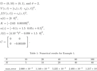
Consider the model state equations representing material balances in the reactor (see [19]) exactly match the mathematical model (1.1) with:
Ω = (0,10)×(0,1),and ϑ = 2,
V(z, t) = [cx(z, t) cy(z, t)]T,
f(V(z, t)) =cx(z, t)2,
u(t) = [0 0]T,
K = [−2.63 0.00109]T,
α(z) = [−0.1z+ 1.5 0.05z+ 0.5]T,
β(t) = [4.10−3t2−0.09t+ 1.5 0]T,
C =
0 0
0 −0.00109
.
Table 1: Numerical results for Example 1.
N 10 20 40 80 160
M 5 10 20 40 80
max error 2.660×10⁻² 1.140×10⁻² 5.225×10⁻³ 2.493×10⁻³ 1.217×10⁻³
Table 1 shows values of the maximum error (max error) obtained in our numerical experiments for different values ofN, andM, we note the convergence of the solutionSto the functionV depends on the discretization parameters h, and ∆t. Theorem 3.4 is shown the convergence of the method provided that the parameters h and ∆t satisfy the relation (3.11). Moreover, the numerical error estimates behave like which confirms what we are expecting.
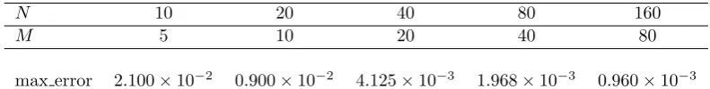
4.2. Example 2: nonisothermal plug flow reactor
Consider the mathematical model of the plug flow reactor (see [2]) exactly matches the mathematical model (1.1) with:
Ω = (0,10)×(0,1) and ϑ= 2,
V(z, t) = [cx(z, t) T(z, t)]T,
f(V(z, t)) = 5.1012c
x(z, t),
u(t) = [0.01 74585.07455507456]T,
K = [−1 −17065.897]T,
α(z) = [0.5 300]T,
β(t) = [0.5 sin(0.1t+ 2000) + 2 0.1625t+ 300]T,
C =
−0.1 0
0 −240.6002405002405
Table 2: Numerical results for Example 2.
N 10 20 40 80 160
M 5 10 20 40 80
max error 2.100×10⁻² 0.900×10⁻² 4.125×10⁻³ 1.968×10⁻³ 0.960×10⁻³
Table 2 shows values of the maximum error (max error) obtained in our numerical experiments for different values ofN andM, we note the convergence of the solution Sto the functionV depends on the discretization parameters h and ∆t. Theorem 3.4 is shown the convergence of the method provided that the parameters h and ∆t satisfy the relation (3.11). Moreover, the numerical error estimates behave like which confirms what we are expecting.
5. Conclusion
In this paper, a quadratic spline collocation approach is prosed in the context to be used for reducing a nonlinear PDEs plug flow reactors models for numerical simulation and/or control design. After a brief review of the nonlinear tubular reactor model in consideration, we present the details of our methodology which consists of first discretizing in time (by Crank-Nicolson scheme) and then collocating in space (by a quadratic spline collocation method). The two test problems which are studied in this paper demonstrate that this approach is an efficient alternative and confirm the theoretical behavior of the rates of convergence.
References
[1] N. Barje, M.E. Achhab and V. Wertz, Observer Design for a class of Exothermal Pug-Flow Tubular Reactors, Int. J. Appl. Math. Research 2 (2013) 273–282.
[2] P.D. Christofides and P. Daoutidis,Robust control of hyperbolic PDE systems. Chem. Engin. Sci. 53 (1998) 85–105. [3] P.D. Christofides,Nonlinear and robust control of the PDE systems: Methods and application to transport-reactor
processs. Boston: Birkh¨auser, 2001.
[4] C.Clavero, J.C. Jorge and F. Lisbona,Uniformly convergent schemes for singular perturbation problems combin-ing alternatcombin-ing directions and exponential fittcombin-ing techniques, in: J.J.H. Miller (Ed.), Applications of Advanced Computational Methods for Boundary and Interior Layers, Boole, Dublin, (1993) pp. 33–52.
[5] C.Clavero, J.C. Jorge, F,Lisbona,A uniformly convergent scheme on a nonuniform mesh for convection-diffusion parabolic problems, J. Comput. Appl. Math. 154 (2003) 415–429.
[6] R.A. DeVore and G.G. Lorentz,Constructive approximation, Springer-Verlag, Berlin, 1993. [7] B.A. Finlayson,Nonlinear Analysis in Chemical Engineering, New York: McGraw-Hill, 1980.
[8] A. Friedman, Partial Differential Equation of Parabolic Type, Robert E. Krieger Publiching Co., Huntington, NY, 1983.
[9] E.A. Garnica, J.P.G. Sandoval and C. Gonzalez-Figueredo, A robust monitoring tool for distributed parameter plug flow reactos, Comput. Chem. Engin. 35 (2011) 510–518.
[10] M. . Kadalbajoo, L.P. Tripathi and A. Kumar,A cubic B-spline collocation method for a numerical solution of the generalized Black-Scholes equation, Math. Comput. Model. 55 (2012) 1483–1505.
[11] O.A. Ladyzenskaja, V.A, Solonnikov and N.N. Ural’ceva, Linear and Quasilinear Equations of Parabolic Type, In: Amer. Math. Soc. Transl., Vol. 23 (1968) Providence, RI.
[12] H.H. Lou, J. Chandrasekaran and R.A. Smith, Large-scale dynamic simulation for security assessment of an ethylene oxide manufacturing process, Comput. Chem. Engin. 30 (2006) 1102–1118.
[13] E. Mermri, A. Serghini, A. El hajaji and K. Hilal, A Cubic Spline Method for Solving a Unilateral Obstacle Problem, Amer. J. Comput. Math. 2 (2012) 217–222.
[15] R.G., Rice and D.D. Do,Applied mathematics and modeling for chemical engineers, New York: John Wiley and Sons Inc., 1995.
[16] P. Sablonnire,Univariate spline quasi-interpolants and applications to numerical analysis, Rend. Sem. Mat. Univ. Pol. Torino 63 (2005) 211–222.
[17] F. Sandelin, P. Oinas, T. Salmi, J. Paloniemi and H. Haario,Dynamic modelling of catalytic liquid-phase reactions in fixed beds-kinetics and catalyst deactivation in the recovery of anthraquinones, Chem. Engin. Sci. 61 (2006) 4528–4539.
[18] J. Villadsen, and M.L. Michelsen,Solution of differential equation models by polynomial approximation. Englewood Cliffs, NJ: Prentice-Hall, 1987.