TDARMA Model Estimation Using the MLS
and the TF Distribution
Abdullah I. Al-Shoshan
Computer Engineering Dept., Qassim University P.O. Box 6688, Qassim 51452, Saudi Arabia
Abstract
An approach for modeling linear time-dependent auto-regressive moving-average (TDARMA) systems using the time-frequency (TF) distribution is presented. The proposed method leads to an extension of several well-known techniques of linear time-invariant (LTI) systems to process the linear, time-varying (LTV) case. It can also be applied in the modeling of non-stationary signals. In this paper, the well-known modified least square (MLS) and the Durbin's approximation methods are adapted to this non-stationary context. A simple relationship between the generalized transfer function and the time-dependent parameters of the LTV system is derived and computer simulation illustrating the effectiveness of our method is presented, considering that the output of the LTV system is corrupted by additive noise.
1
Introduction
Linear systems (Mullis, 1976) serve as basic tools in various fundamental areas and the problems of system identification and signal modeling have attracted considerable attention due to their large number of applications in diverse fields(Astrom, 1971)(Al-Shoshan, 1996), (Broersen, 2000), (Choi, 1992),(Lobato, 2018), (Diggle, P. J., 1990), (Grenier, 1983), (Wood, 1992). The time-invariant case, where the signals are stationary and the system's operations are steady, is well established. In this case, the representation of the signals and the characterization and design of the systems are conducted in either the time or the frequency domain (Haykin, 1991), (Huang, 1980), (Ding F. X., 2016). Whenever the signal of interest or the desired system operations are non-stationary, such approaches are quite limited, see for example (Kayhan, 1994), (Kenny, 1993), as they do not often express explicitly the signal or system non-stationarity. Whenever slow temporal variations are presumed, the problem is resolvable by partitioning the signal into time sections that are sufficiently small to be considered locally time-invariant and sufficiently long to yield the desired frequency resolution. In this paper, we will develop some tools for dealing with LTV systems and non-stationary signals without the above assumptions.
Volume 58, 2019, Pages 282–291
1.1
Time-Frequency Distributions
An accurate spectral analysis of nonstationary signals cannot be accomplished by the simple use of classical time-domain or frequency-domain representation. To deal with time-dependent spectrum, the concept of time-frequency distributions has been introduced. These methods represent an attempt to provide a general solution to the problem of representing non-stationary signals. In order to develop a useful theory we need to replace stationarity by a more general notion, which still allows us to carry out meaningful statistical analysis and to develop a form of time-dependent spectral analysis, which shares many of the features of the spectral analysis of stationary processes (Priestley, 1988). The Short-Time Fourier Transform (STFT) (Portnoff, 1980), the Wigner Distribution (WD) (Haykin, 1991), the Wavelet Transform (WT) (Rioul, 1991), the Evolutionary Periodogram (EP) (Kayhan, 1994), and the Minimum-Cross Entropy (MCE) (Loughlin, 1994) are some fundamental examples of estimators using the concept of Time-Frequency Distributions (TFD) (Pincinbono, 1989). In this paper, we have used the evolutionary periodogram (EP), developed by (Kayhan, 1994). For a nonstationary signal x(n), the EP is expressed as follows:
jwm n
N
m
e
m
x
m
w
w
n
H
(
)
(
)
=
)
,
(
ˆ
10 =
(1)
where
)
(
)
(
=
)
(
*1
0 =
m
n
m
w
i iM
i
n
(2)
is a time-varying window and {βi(n)} is a set of orthonormal polynomials on nϵ[0, N-1].
1.2
LTV Systems
A simple remedy for dealing with LTV system is to write the model parameters in each effective data window as a linear sum of some known time functions. In this case, each time-dependent model parameter (Rao, 1970) is replaced with a constant parameter vector that is made up of the constant parameters in the linear sum of the known time functions. In this paper, we will consider a more general case. In the time domain, the input/output behavior of an LTV system can be characterized by a weighting pattern, or Green’sfunction, g(n,m), which represents the response of the system at discrete-time n to a unit-impulse applied at discrete-time m. Equivalently, the same system can be described by a time-varying unit-impulse response ζ(n,m) defined as the response of the system at time n to a unit-impulse applied m samples earlier, i.e., at time (n-m). Furthermore, the time-varying unit-impulse response ζ(n,m) and the Green’sfunctiong(n,m) are related by , (Broersen, 2000) ζ(n,m)=g(n,n-m) or equivalently, g(n,m)=ζ(n,n-m). If y(n) is the response of a causal LTV rational system with impulse response ζ(n,m) to an input x(n), then y(n) is given by the superposition sum
) ( ) ( ) ( ) ( ) ( =
) ( ) ( ) , ( = ) (
1 = 0
= =
n k n y n a k n x n b
n m n x m n n
y
k p
k k
q
k n
m
where η(n) is a white noise at the system output, x(n) is a stationary input signal, and {ak(n)} and {bk(n)} are sets of time-dependent parameters, p ≥ q, a0(n)=1. If the system represented by ζ(n,m) is
time-invariant, then ζ(n,m) depends only on the difference (n-m) corresponding to the number of samples between the application of the unit impulse and the observation of the output; thus, ζ(n,m)=g(n,n-m)=g(n-(n-m)=g(m)=ζ(m) and corresponds to the ordinary unit-impulse response of such a system, so equation (3) reduces to
)
(
)
(
)
(
=
)
(
)
(
)
(
=
)
(
1 = 0
= =
n
k
n
y
a
k
n
x
b
n
m
n
x
m
n
y
k p
k k
q
k n
m
(4)
which represents the response and difference equation of an LTI system. Assuming for instance that η(n)=0, from equation (4), we have
0 = ) ( ) ( ) ( ) ( =
) ( ) ( ) , (
0 = 0
= =
k n y n a k n x n b
n y m n x m n
k p
k k
q
k n
m
(5)
which shows a relationship between the system response ζ(n,m) and the time-dependent coefficients {ak(n)} and {bk(n)} of the system difference equation. In section 2, we discuss the identification of the time-dependent parameters of a rational LTV system and propose a relationship between the generalized transfer function Γ(n,z) of the LTV system and the time-dependent coefficients {ak(n)} and {bk(n)} of its difference equation. Also, modifications of the MLS and the Durbin's approximation methods are proposed. Simulation examples showing the performance of the proposed method are presented in Section 3, and we conclude our results in Section 4.
2
TDARMA Modeling Using the TD Parameters and the
Generalized Transfer Function
) ( ] ) ( [
) ( ] ) ( [ = ) ( ) , ( ) (
0 =
0 =
z Y z n a
z X z n b z Y z n z X
k k p
k
k k q
k
(6)
and hence
k k p
k
k k q
k
z
n
a
z
n
b
z
n
A
z
n
B
z
n
)
(
)
(
=
)
,
(
)
,
(
=
)
,
(
0 =
0
= (7)
where Γ(n,z) represents the generalized transfer function of the LTV system (Astrom, 1971), or the z -transform of ζ(n,m) with respect to m. Equation (7) represents a simple relationship between the time-dependent coefficients of the difference equation of the LTV system {ak(n)} and {bk(n)} and its time-varying impulse response ζ(n,m). When x(n) is a non-Gaussian process, but the noise η(n) has still Gaussian distribution, one can reduce the effect of noise by using the method proposed in (Broersen, 2000). The time-varying system impulse response ζ(n,m) can be estimated by first estimating the time-varying frequency response (or the generalized transfer function) Γ(n,ω) using any time-frequency kernel estimator to get Γ(n,ω) and its corresponding inverse Fourier transform ζ(n,m). From
ˆ(n,m), which is the estimate of ζ(n,m), we estimate the time-dependent coefficients of the LTV system.2.1
Estimating the TD-AR Parameters
To solve for the autoregressive parameters (AR) {ak(n)} of the LTV system described by (7), the modified least-square (MLS) method (Broersen, 2000), (Landers, 1977) and (Ding F. M., 2018) is adapted. In the MLS a rational function that approximately has {ζ(n,m)} as its impulse response, using the MLS minimization problem is obtained. The mean square error in the AR model is a quadratic form of the time-dependent parameters and its minimization leads to a set of linear equations, as in the stationary case. From equation (7), we have Γ(n,k)A(n,k)=B(n,k). Therefore, we will try to find the parameters of a rational function that approximates the above equation by minimizing the following quadratic error
2 1
0 = 2
|
)
,
(
)
,
(
)
,
(
|
=
n
k
A
n
k
B
n
k
N
k
n
(8)where N is the number of samples in time-domain. The solution of this problem can be obtained by recursively solving the system of time-dependent linear equations
t p
t p
n
a
n
a
n
n
K
[1,
1(
),...,
(
)]
=
[
(
),0,...,0]
(9)
) , min( 0 *|)
|
,
(
)
,
(
|)
(|
)
,
(
j i p qm y y
n
n
i
j
r
i
j
n
m
n
m
i
j
K
(10)where i, j=0, 1, ..., p, and
p(
n
)
is the time-varying minimization error for A(n,z) of order p. The entries of the(
p
1)
(
p
1)
time-dependent matrix Kn are given by)
,
(
)
,
(
)
(
=
)
,
(
* ) , ( 0 =l
m
n
m
n
l
r
j
i
K
j i min p q m nn
(11)where l=|i-j|, i, j= 0, 1, …, p, ζ(n,m) is the impulse response sequence of the LTV system and rn(m) is the time-varying autocorrelation function (TVACF) of y(n). The TVAR parameters can then be computed from equation (9) as
t p
n t
p
n
K
n
a
n
a
(
),...,
(
)]
=
[
(
),0,...,0]
[1,
1 1
(12)
2.2
Estimating the TDMA Parameters
The identification of the TDMA part is much more difficult because it is a non-linear problem. In this paper, the Durbin's approximation method is modified for the estimation of the TDMA parameters by considering the time-varying autocorrelation function proposed in (Astrom, 1971) and (Liporace, 1975). The TDMA parameters can be obtained by approximating the low-order MA model by a high-order AR model. After obtaining the TDAR parameters, one can form an equivalent TDMA model by removing the TDAR component as follows. Assuming there is no noise in the output, equation (3) can be rewritten as
)
(
)
(
)
(
~
=
)
(
1 =i
n
y
n
a
n
y
n
y
i p i
(13)where
~
y
(
n
)
can be considered as the output of an equivalent TDMA model represented by)
(
)
(
=
)
(
~
0 =i
n
x
i
n
b
n
y
i q i
(14)Taking the autocorrelation of the sequence in equation (10), we have
)}
(
)
(
{
)
(
)
(
=
)}
(
~
)
(
~
{
=
)
(
* * 0 = 0 = * ~j
m
n
x
i
n
x
E
j
m
n
b
i
n
b
m
n
y
n
y
E
m
r
j i q j q i y n
(15))
(
)
(
=
)
(
* 0 = 0 = ~j
m
n
b
i
n
b
m
r
i jq
j q
i y
n
(16)where m=0, 1, …, q. The problem now is to estimate {bi(n)} from the time-varying autocorrelation
function
r
n~y(
m
)
of the MA sequence~
y
(
n
)
. Equation (15) is nonlinear and, in general, does not have a unique solution. However, at each instant of time n, {bi(n)} can be estimated by modifying the Durbin's approximation method for the estimation of the MA parameters of an MA(q) process. Using the data sequence{
~
y
(0),
~
y
(1),...,
~
y
(
N
1)}
, fit a large order AR model using the autocorrelation method. For an AR model order L, where q<<L<<N, the white noise variance estimator
~
n2 is given by)
(
~
)
(
~
(0)
~
=
~
~ 1 = ~ 2k
r
k
a
r
n nyL
k y n
n
(17)and from
{
a
~
n(1),
a
~
n(2),...,
~
a
n(
L
)}
, we use the autocorrelation method with order of q to find )} ( ~ (2),..., ~ (1), ~ { = ~ L b b bbn n n n as b~n=R~n1~rn where
|)
|
(
~
)
(
~
1
1
=
]
~
[
* | | 0 =j
i
k
a
k
a
L
R
n nj i L
k ij
n
(18) and
)
(
~
)
(
~
1
1
=
]
~
[
* | 0 =i
k
a
k
a
L
r
n ni L
k i
n
(19)
{bk(n)} can also be estimated from {aˆk(n)} and the time-varying impulse response
ˆ
(
n
,
m
)
of the time-varying system as)
,
(
)
(
=
)
(
0 =j
k
n
n
a
n
b
j p jk
(20)where k=0, 1, …, q, and the accuracy of the estimated time-dependent coefficients depends on how good is the estimate ˆ(n,) of Γ(n,ω).
3
Simulations and Results
Example 1: Consider a non-stationary signal generated from a second-order TDARMA(p,q) model such that p=2, q=0 in equation (3), i.e., y(n)=x(n)-a1(n)y(n-1)-a2(n)y(n-2), where
N n N
N n N
n
n a
< 2 0.5
2 < 0 = ) ( 1
,
N n N N n
N n n
a
< 2 1
2 < 0 0.5 = ) ( 2
with n=0, 1, …, N-1, and N=64, assuming there is no noise, i.e., η(n)=0 in equation (3) and the input x(n) is a zero-mean, unit-variance stationary white noise. Using 60 Monte-Carlos, the true and the estimated coefficients
a
ˆ
1(
n
)
anda
ˆ
2(
n
)
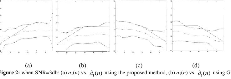
of the LTV system are shown in Figure 1(a) and (c) using the proposed method, compared with Figure 1(b) and (d) using the geometric lattice (GL) method, respectively. We observe from the figures that the estimated coefficients are tracking the actual ones in both methods, however, the proposed one tracks better. Also, the standard deviation is better in the proposed method. Adding a Gaussian noise with SNR=3db to the system output, we get the results shown in Figure 2. Although both methods track the actual parameters, both of them are degraded by noise.(a) (b) (c) (d) Figure 1: (a) a1(n) vs. ˆ( )
1 n
a using the proposed method, (b) a1(n) vs. ˆ( ) 1 n
a using GL method, (c) a2(n) vs.
) ( ˆ2 n
a using the proposed method, (d) a2(n) vs. aˆ2(n) using GL method
(a) (b) (c) (d) Figure 2: when SNR=3db: (a) a1(n) vs. ˆ( )
1n
a using the proposed method, (b) a1(n) vs. ˆ( )
1 n
a using GL method, (c) a2(n) vs. ˆ ( )
2 n
a using the proposed method, (d) a2(n) vs. ˆ ( ) 2 n
a using GL method
Example 2: In this example we consider a TDARMA(p,q) model, with p=2 and q=1. If we let y(n)=b(n)x(n)-a1(n)y(n-1)-a2(n)y(n-2), where a1(n)=sin(3.15n/N), a2(n)=0.5(1-cos(3n/N)), and
Monte-) ( ˆ1 n
a and aˆ2(n) for the proposed method, compared with Figure 3(b) and (d) using the geometric lattice method, respectively. Figure 4 shows the TDMA part of both methods. We also observe here that the estimated coefficients are tracking the actual ones in both methods, however, the proposed one tracks better. Also, the standard deviation is better in the proposed method than that of the geometric lattice one. Adding a Gaussian noise with SNR=3db to the system output, we get the results shown in Figure 5 and Figure 6 for the TDAR and the TDMA parameters, respectively. We observe from the figures that the estimated coefficients are still tracking the actual ones even if the system output is corrupted by noise. We also observe here that although both methods still track the actual parameters, both of them are degraded by noise.
(a) (b) (c) (d) Figure 3: (a) a1(n) vs. ˆ( )
1 n
a using the proposed method, (b) a1(n) vs. ˆ( )
1n
a using GL method, (c) a2(n) vs.
) ( ˆ2 n
a using the proposed method, (d) a2(n) vs. aˆ2(n) using GL method
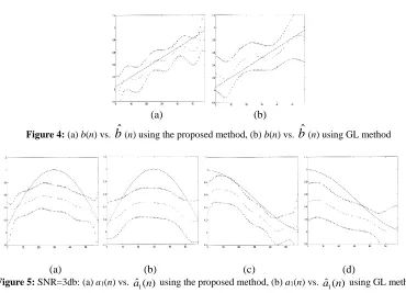
(a) (b)
Figure 4: (a) b(n) vs.
b
ˆ
(n) using the proposed method, (b) b(n) vs.b
ˆ
(n) using GL method(a) (b) (c) (d) Figure 5: SNR=3db: (a) a1(n) vs. ˆ( )
1n
a using the proposed method, (b) a1(n) vs. ˆ( )
1n
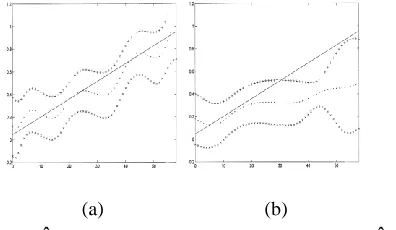
(a) (b)
Figure 6: SNR=3db: (a) b(n) vs.
b
ˆ
(n) using the proposed method, (b) b(n) vs.b
ˆ
(n) using GL method4
Conclusions
In this paper, the problem of identification and modeling of a TDARMA system is addressed. An approach for parameters estimation based on the superposition representation of non-stationary signals is presented. This approach has an advantage that the parameters are computed using a set of linear equations. The MLS and the Durbin's approximation methods were adapted and modified to the non-stationary context using the TF distribution. It has also been demonstrated through computer simulations that when the system output is corrupted by a Gaussian noise, the proposed method performs well in the modeling process.
References
Al-Shoshan, A. I. (1996). Identification of Non-minimum Phase Systems Using the Evolutionary Spectral Theory. Signal Processing Journal, 55, 79-92.
Astrom, K. J. (1971). System Identification - A Survey. Automatica, 7, 123-162.
Broersen, P. M. (2000). Autoregressive Model Orders for Durbin's MA and ARMA Estimators. IEEE Trans. Signal Processing, 48(8), 2454-2457.
Choi, B. S. (1992). ARMA Model Identification. NY: Springer-Verlag.
Diggle, P. J. (1990). Time Series: A Biostatistical Introduction. Oxford: Oxford University Press. Ding, F. M. (2018). Least Squares based Iterative Parameter Estimation Algorithm for Stochastic
Dynamical Systems with ARMA Noise Using the Model Equivalence. Int. J. Control Autom. Syst., 16 (2), 630–639.
Ding, F. X. (2016, December). Performance analysis of the generalised projection identification for time-varying systems. IET Control Theory and Applications, 10(18), 2506–2514.
Grenier, Y. (1983). Time-Dependent ARMA Modeling of Non-stationary Signals. IEEE Trans. on ASSP, 31(4), 899-911.
Haykin, S. (1991). Advances in Spectrum Analysis and Array Processing. Englewood Cliffs, NJ:Prentice-Hall.
Huang, N. C. (1980). On Linear Shift-Variant Digital Filters. IEEE Trans. on Circuits and Systems, 27(8), 672-679.
Kayhan, A. E.-J. (1994, June). Evolutionary Periodogram for Non-Stationary Signals,. IEEE Trans. on Signal Proc., 42, 1527-1536.
Landers, T. E. (1977). Some Geophysical Applications of Autoregressive Spectral Estimates. IEEE Trans. on Geoscience Electronics, 15, 26-32.
Liporace, L. A. (1975, Dec). Linear Estimation of Nonstationary Signals. J. Acoustics Soc. of Am, 58, 1288-1295.
Lobato, I. N. (2018). Efficiency improvements for minimum distance estimation of causal and invertible ARMA models. Economics Letters, 162, 150-152.
Loughlin, P. P. (1994, Oct). Construction of Positive Time-Frequency Distributions. IEEE Trans. Sig. Proc., 42(10), 2697-2705.
Mullis, C. T. (1976, June). The Use of Second-Order Information in the Approximation of Discrete-Time Linear Systems. IEEE Trans. on ASSP, 24(3), 226-238.
Pincinbono, B. (1989). , ed., Time and Frequency Representation of Signals and Systems. NY: Springer:NY.
Portnoff, M. R. (1980, Feb.). , “Time-Frequency Representation of Digital Signals and Systems Based on Short-Time Fourier Analysis. IEEE Trans. Acoustic, Speech, Signal Processing, 28(1), 681-684.
Priestley, M. B. (1988). Non-linear and Non-stationary Time Series Analysis. New York: NY:Academic Press.
Rao, S. T. (1970, Mar). The fitting of Nonstationary Time Series Models with Time-Dependent Parameters. J. Stat. Soc., 32(Ser. B), 312-322.
Rioul, O. a. (1991, October). Wavelets and Signal Processing. IEEE Signal Processing Magazine, 14-38.