OPTIMIZATION OF RENEWAL INPUT (a, c, b) POLICY WORKING VACATION QUEUE WITH CHANGE OVER TIME AND BERNOULLI
SCHEDULE VACATION INTERRUPTION
P. VIJAYA LAXMI1, V. GOSWAMI2, D. SELESHI1,§
Abstract. This paper presents a renewal input single working vacation queue with change over time and Bernoulli schedule vacation interruption under (a, c, b) policy. The service and vacation times are exponentially distributed. The server begins service if there are at least c units in the queue and the service takes place in batches with a minimum of sizeaand a maximum of sizeb(a≤c≤b). The change over period follows if there are (a−1) customers at service completion instants. The steady state queue length distributions at arbitrary and pre-arrival epochs are obtained. An optimal cost policy is presented along with few numerical experiences. The genetic algorithm and quadratic fit search method are employed to search for optimal values of some important parameters of the system.
Keywords: Single working vacation, vacation interruption, cost, queue, genetic algorithm.
AMS Subject Classification: Primary 60K25; Secondary 90B22, 68M20.
1. Introduction
Working vacation (WV) models are widely used to analyze many problems in the area of computer communication, manufacturing, production and transportation systems. In these models service is provided during vacation at a rate usually lower than the regular service rate. The concept was introduced by Servi and Finn [1] while analyzing anM/M/1 queue with multiple working vacation (MWV), which was extended to GI/M/1/M W V
queue by Baba [2]. For single working vacation (SWV) queues, Chae et al. [3] considered theGI/M/1 and GI/Geo/1 queues. The performance analysis of a GI/M/1 queue with SWV has been studied by Li and Tian [4]. Further studies on WV are found in Banik et al. [5], Goswami and Mund [6], Jain and Singh [7], Li et al. [8], Tian and Zhang [9], etc.
Li and Tian [10] first introduced an vacation interruption (VI) in an M/M/1 queue. Later, Li et al. [11] generalized their results to aGI/M/1 queue with WV and VI. Zhao et al. [12] studied aGI/M/1 queue with set-up period, WV and VI. A WV queue with service interruption and multi optional repair was discussed by Jain et al. [13]. Zhang and Hou [14] analyzed aM AP/G/1 queue with WV and VI. For the Bernoulli schedule vacation interruption (BS-VI), Zhang and Shi [15] first studied anM/M/1 queue with VI under the Bernoulli rule. Recently, Li et al. [16] studied a GI/Geo/1 SWV queue with
1 Department of Applied Mathematics, Andhra University, Visakhapatnam 530 003, India.
e-mail: vijaya [email protected]; seleshi [email protected];
2 School of Computer Application, KIIT University, Bhubaneswar 751024, India.
e-mail: veena [email protected]; § Manuscript received: September 12, 2013.
TWMS Journal of Applied and Engineering Mathematics, Vol.4, No.2; c⃝I¸sık University, Department of Mathematics, 2014; all rights reserved.
start-up period and BS-VI using embedded Markov chain technique. Further, see Gao and Liu [17] for a study onM/G/1 queue with SWV and BS-VI.
In many real-life queueing situations jobs are served with a control limit policy. For ex-ample, in some manufacturing systems it is possible to process jobs only when the number of units to be processed exceeds a specified level, and when service starts, it is profitable to continue it even when the queue size is less than the specified level but not less than a secondary limit. Tadj et al. [18] have analyzed an optimal control of batch arrival, bulk service queueing system withN policy. The infinite buffer multiple vacations queue with change over times under (a, c, d) policy has been studied by Baburaj and Surendranath [19], where the arrivals and service times are exponentially distributed. A discrete time bulk service (a, c, d) policy queue has been presented by Baburaj [20].
One of the most fundamental objectives in the performance evaluation of queueing mod-els is to search for an optimal value. Many practical design problems are characterized by mixing continuous and discrete variables, discontinuous and non-convex design spaces. In such cases, the standard non linear optimization techniques will be inefficient, computa-tionally expensive, and in most cases, find relative optimum that is closest to the starting point. Genetic algorithm (GA) is well suited for solving such problems and in most cases it finds the global optimum solution with high probability. More details on GA can be found in Haupt & Haupt [21], Lin and Ke ([22], [23]), Rao [24], etc.
Quadratic fit search method (QFSM) is another optimization technique which can be used when the objective function is highly complex and obtaining its derivative is a diffi-cult task. Given a 3-point pattern, one can fit a quadratic function through corresponding functional values that has a unique optimum for the given objective function. For details of QFSM one may refer Rardin [25].
Motivated by the problem of optimization in an (a, c, b) policy queue with vacations, this paper focuses on an infinite buffer renewal input SWV queue with change over time and BS-VI under (a, c, b) policy. The inter-arrival time of customers and service time of batches are respectively, arbitrarily and exponentially distributed. We provide a recursive method using the supplementary variable technique to develop the steady state queue length distributions. Various performance measures and a cost model are developed to determine the optimum service rates in regular busy period and in working vacation, using GA and QFSM. Numerical results are presented to show the effect of model parameters.
The rest of the paper is organized as follows. Model description is given in Section 2. Section 3 presents the computations of the steady state distributions of the number of customers in the queue at arbitrary and pre-arrival epochs. Section 4 discusses various performance measures and the cost analysis. Section 5 contains numerical results and Section 6 concludes the paper.
2. Description of the model
We consider a SWV GI/M(a,c,b)/1 queueing system with change over time and BS-VI. It is assumed that the inter-arrival times of customers are independent and identically dis-tributed random variables with cumulative distribution functionA(x), probability density function a(x), x ≥ 0, Laplace-Stiltjes transform (L.-S.T.) A∗(θ), Re(θ) ≥ 0 and mean inter-arrival time 1/λ =−A∗(1)(0), where h(1)(x0) denotes the first derivative of h(x) at
x=x0. The service begins only if there are at leastc units in the queue. The customers are served in batches with minimum sizeaand maximum size b(a≤c≤b). The various server states and the activities are given below: At a service completion epoch during regular busy period if the queue size (j) is
• 0≤j≤a−2 : the server goes for WV.
• j = a−1 : server will wait for some time in the system called change over time which is exponentially distributed with rate α. It starts service on finding an arrival during this change over time, otherwise it will go for WV.
On returning from working vacation, if the queue sizej is
• 0 ≤ j ≤ c−1 : the server remains dormant in the system until c customers are available in the queue.
• j≥c: min{j, b} customers are served according to first-come, first-served rule. Service times during regular busy period, during vacation and vacation times are exponen-tially distributed with rateµ,η and ϕ, respectively. During a WV a customer is serviced at a lower rate and at the instants of a service completion, the vacation is interrupted and the server is resumed to a regular busy period with probability ¯q = 1−q (if there are at leastccustomers in the queue), or continues the vacation with probability q. Further, the inter-arrival times, service times, change over times and WV times are mutually indepen-dent of each other. The traffic intensity is given byρ=λ/bµ. The state of the system at timetis described by the following random variables:
• X(t) = number of customers present in the queue, • U(t) = remaining inter-arrival time for the next arrival,
• Y(t) =
0, if the server is in working vacation,
1, if the server is busy,
2, if the server is in change over time,
3, if the server is dormant.
At steady state, let us define
Pn,j(x)dx = lim
t→∞P r
{
X(t) =n, x < U(t)≤x+dx, Y(t) =j }
, j = 0,1,2,3.
LetPn,∗0(θ), Pn,∗1(θ), Pn,∗2(θ) andPn,∗3(θ) be the L.-S.T. of Pn,0(x), Pn,1(x), Pn,2(x) and
Pn,3(x), respectively so that Pn,0 ≡ Pn,∗0(0), n ≥ 0, Pn,1 ≡ Pn,∗1(0), n ≥ 0, Pn,2 ≡
Pn,∗2(0), n = a−1 and Pn,3 ≡ Pn,∗3(0), 0 ≤n ≤ c−1 are the steady state probabilities that n customers are in the queue and the server is in working vacation, regular busy period, in change over time and dormancy, respectively, at an arbitrary epoch.
3. Analysis of the model
In this section, we shall discuss the steady state queue length distributions using the supplementary variable technique and the recursive method. We first establish the math-ematical equations that govern the system by employing the remaining inter-arrival time as the supplementary variable. Relating the states of the system at two consecutive time epochstandt+dt, and using probabilistic arguments, we set up the following differential-difference equations at steady state:
−P0(1),0(x) = µP0,1(x) +qη b
∑
n=c
Pn,0(x)−ϕP0,0(x),
−Pn,(1)0(x) = a(x)Pn−1,0(0) +µPn,1(x) +qηPn+b,0(x)−ϕPn,0(x), 1≤n≤a−2, −Pa(1)−1,0(x) = a(x)Pa−2,0(0) +αPa−1,2(x) +qηPa+b−1,0(x)−ϕPa−1,0(x),
−P0(1),1(x) = a(x)Pa−1,2(0) +a(x)Pc−1,3(0) +µ
b
∑
n=a
Pn,1(x) + (ϕ+ ¯qη)
b
∑
n=c
Pn,0(x) −µP0,1(x),
−Pn,(1)1(x) = a(x)Pn−1,1(0) +µPn+b,1(x) + (ϕ+ ¯qη)Pn+b,0(x)−µPn,1(x), n≥1, −Pa(1)−1,2(x) = µPa−1,1(x)−αPa−1,2(x),
−P0(1),3(x) = ϕP0,0(x),
−Pn,(1)3(x) = a(x)Pn−1,3(0) +ϕPn,0(x),1≤n≤c−1.
where Pn,j(0), n ≥ 0, j = 0,1,2,3 are the respective probabilities with the remaining
inter-arrival time equal to zero, i.e., an arrival is about to occur. Multiplying the above equations bye−θx, integrating with respect to x from 0 to∞ yields
(ϕ−θ)P0∗,0(θ) = µP0∗,1(θ) +qη
b
∑
n=c
Pn,∗0(θ)−P0,0(0), (1)
(ϕ−θ)Pn,∗0(θ) = A∗(θ)Pn−1,0(0) +µPn,∗1(θ) +qηPn∗+b,0(θ)−Pn,0(0),
1≤n≤a−2, (2)
(ϕ−θ)Pa∗−1,0(θ) = A∗(θ)Pa−2,0(0) +αPa∗−1,2(θ) +qηPa∗+b−1,0(θ)−Pa−1,0(0), (3) (ϕ−θ)Pn,∗0(θ) = A∗(θ)Pn−1,0(0) +qηPn∗+b,0(θ)−Pn,0(0), a≤n≤c−1, (4)
(η+ϕ−θ)Pn,∗0(θ) = A∗(θ)Pn−1,0(0) +qηPn∗+b,0(θ)−Pn,0(0), n≥c, (5)
(µ−θ)P0∗,1(θ) = A∗(θ)Pa−1,2(0) +A∗(θ)Pc−1,3(0) +µ
b
∑
n=a
Pn,∗1(θ)
+(ϕ+ ¯qη)
b
∑
n=c
Pn,∗0(θ)−P0,1(0), (6) (µ−θ)Pn,∗1(θ) = A∗(θ)Pn−1,1(0) +µPn∗+b,1(θ) + (ϕ+ ¯qη)Pn∗+b,0(θ)−Pn,1(0),
n≥1, (7)
(α−θ)Pa∗−1,2(θ) = µPa∗−1,1(θ)−Pa−1,2(0), (8)
−θP0∗,3(θ) = ϕP0∗,0(θ)−P0,3(0), (9)
−θPn,∗3(θ) = A∗(θ)Pn−1,3(0) +ϕPn,∗0(θ)−Pn,3(0), 1≤n≤c−1. (10)
Adding equations (1) to (10), taking limit asθ→0 and using the normalizing condition,
∑∞
n=0(Pn,0+Pn,1) +Pa−1,2+
c∑−1
n=0
Pn,3 = 1, we obtain ∞
∑
n=0
(
Pn,0(0) +Pn,1(0)
)
+Pa−1,2(0) + c−1
∑
n=0
Pn,3(0) =λ. (11)
It may be noted here that the left-hand side of (11) represents the probability that an arrival is about to occur, which is equal to the arrival rate of customers. This is used in the sequel to obtain a relation between an arrival is about to occur and the pre-arrival epoch probabilities.
and the server is in statej at arrival epochs. Applying Bayes’ theorem, we have
Pn,j− = lim
t→∞
P[X(t) =n, Y(t) =j, U(t) = 0]
P[U(t) = 0] . Further, using (11) in the above expression, we obtain
Pn,j− = 1
λPn,j(0), n≥0, j = 0,1; n=a−1, j = 2; 0≤n≤c−1, j = 3. (12)
To obtainPn,j− , we need to evaluatePn,j(0), which is discussed below.
We define the displacement operatorE as Exωn=ωn+x, and rewrite equation (5) as
(η+ϕ−θ−qηEb)Pn,∗0(θ) = (A∗(θ)−E)Pn−1,0(0), n≥c.
Settingθ=η+ϕ−qηEb in the above equation, we get
Pn,0(0) =krn, n≥c−1. (13)
wherekis an arbitrary constant and r is a real root inside the unit circle of the equation
A∗(η+ϕ−qηzb)−z= 0. We also have,
Pn,∗0(θ) =g(n, θ)k, n≥c, (14) whereg(n, θ) = rn−1(τA∗(θ)−r)
1−θ and τ1 =η(1−qr
b) +ϕ.
From equation (7), we get
Pn,1(0) = k1ξn−
(ϕ+ ¯qη)krn+b τ2
, n≥0, (15)
Pn,∗1(θ) = g1(n, θ)k1+g2(n, θ)k, n≥1, (16) whereτ2=τ1−µ(1−rb),k1 is an arbitrary constant, ξ is a real root inside the unit circle of the equationA∗(µ−µzb)−z= 0 and
g1(n, θ) =
ξn−1(A∗(θ)−ξ)
µ−θ−µξb ,g2(n, θ) =−
(ϕ+ ¯qη)(A∗(θ)−r)rn+b−1
τ2(τ1−θ)
.
Settingθ=α in equation (8) and using equation (16), one can obtain Pa−1,2(0) as
Pa−1,2(0) =k1L1−kL2, (17) where
L1 =
µ(A∗(α)−ξ)ξa−2
µ−µξb−α and L2 =
µ(A∗(α)−r)(ϕ+ ¯qη)ra+b−2 τ2(τ1−α)
.
Equation (8) together with equations (16) and (17) yields
Pa∗−1,2(θ) =g3(θ)k1+g4(θ)k, (18) where
g3(θ) = 1
α−θ (
µ(A∗(θ)−ξ)ξa−2 µ−µξb−θ −L1
) ,
g4(θ) = 1
α−θ (
L2−
µ(A∗(θ)−r)(ϕ+ ¯qη)ra+b−2 τ2(τ1−θ)
) .
Now insertingθ=ϕand using equations (13) and (14) in equation (4), we get
where
h(n) = A∗(ϕ)n−c+1
(
1− {qη(A∗(ϕ)−r)rb−c+n+1
c−∑n−2
i=0
riA∗(ϕ)c−n−2−i}/(τ1−ϕ)
) .
Settingθ=ϕin (3), we get
Pa−2,0(0) =kL3−k1L4, (20) where
L3 = 1
A∗(ϕ)
(
rc−1h(a−1)− α
α−ϕ (
L2−
µ(A∗(ϕ)−r)(ϕ+ ¯qη)rb+a−2 τ2(τ1−ϕ)
)
−qη(A∗(ϕ)−r)ra+b−2
τ1−ϕ
) ,
L4 =
α A∗(ϕ)(α−ϕ)
(
µ(A∗(ϕ)−ξ)ξa−2 µ−ϕ−µξb −L1
) .
Settingθ=ϕin equation (2), we obtain
Pn,0(0) =kh1(n)−k1h2(n), 0≤n≤a−3, (21) where
h1(n) = A∗(ϕ)n−a+2
( L3+
(A∗(ϕ)−r)rb+n (
µ(ϕ+ ¯qη)−qητ2
)a−∑3−n i=0
riA∗(ϕ)a−3−n−i
τ2(τ1−ϕ)
) ,
h2(n) = A∗(ϕ)n−a+2
( L4+
µ(A∗(ϕ)−ξ)ξn
a−∑3−n i=0
ξiA∗(ϕ)a−3−n−i
µ−ϕ−µξb
) .
Insertingθ=µ in equation (6), we get
Pc−1,3(0) =
k1
A∗(µ)
(
1−A∗(µ)L1+
(A∗(µ)−ξ)(ξa−1−ξb)
ξb(1−ξ)
)
+ k
A∗(µ)
(
A∗(µ)L2 −(ϕ+ ¯qη)rb
τ2
+(A
∗(µ)−r)(ϕ+ ¯qη)(µ(rb+a−1−r2b)−τ
2(rc−1−rb)
)
τ2(τ1−µ)(1−r)
) .
(22) Puttingθ= 0 in equation (6), we get
µP0,1 =k1L5+kL6, (23)
where
L5 = 1
A∗(µ) + (ξ
a−1−ξb)
(
A∗(µ)−ξ A∗(µ)ξb(1−ξ) +
1 1−ξb
)
−1,
L6 =
ϕ+ ¯qη τ2
(
rb(A∗(µ)−1)
A∗(µ) +
[
µ(rb+a−1−r2b)−τ2(rc−1−rb)
]
×
( A∗(µ)−r
A∗(µ)(τ1−µ)(1−r) − 1
τ1
)) .
Settingθ= 0 in equation (1), we obtain
P0,0 =
k1
ϕ (
L5+h2(0)
)
+k
ϕ (
L6+
qη(rc−1−rb)
τ1 −
h1(0)
)
Putθ= 0 in equation (2) to get
Pn,0 = kh3(n) +k1h4(n), 1≤n≤a−3, (25)
Pa−2,0 =
k ϕ
(
h1(a−3)−L3−
(1−r)rb+a−3 (
µ(ϕ+ ¯qη)−qητ2
)
τ2τ1
)
+k1
ϕ
((1−ξ)ξa−3
1−ξb +L4−h2(a−3)
)
, (26)
where
h3(n) = 1
ϕ (
h1(n−1)−h1(n)−
(1−r)rb+n−1 (
µ(ϕ+ ¯qη)−qητ2
)
τ2τ1
) ,
h4(n) = 1
ϕ (
(1−ξ)ξn−1
1−ξb +h2(n)−h2(n−1)
) .
Using equation (3) forθ= 0, we obtain
Pa−1,0 =
k ϕ
(
L3+L2−
(1−r)ra+b−2 (
µ(ϕ+ ¯qη)−qητ2
)
τ2τ1 −
rc−1h(a−1)
)
+k1
ϕ
((1−ξ)ξa−2
1−ξb −L1−L4)
)
. (27)
Insertingθ= 0 in equation (4), we get
Pn,0 =
k ϕ
( rc−1
(
h(n−1)−h(n)
)
+ qη(1−r)r
b+n−1
τ1
)
, a≤n≤c−2, (28)
Pc−1,0 =
krc−1 ϕ
(
h(c−2)−1 +qη(1−r)r
b−1
τ1
)
. (29)
From equations (9) and (10), we get
Pn,3(0) =ϕ
n
∑
j=0
Pj,0, 0≤n≤c−1. Thus using (24) to (28), we have
P0,3(0) = k
( L6+
qη(rc−1−rb)
τ1 −
h1(0)
)
+k1
(
L5+h2(0)
)
, (30)
Pn,3(0) = kh5(n) +k1h6(n), 1≤n≤a−3, (31)
Pa−2,3(0) = k1
(
h6(a−3) +(1−ξ)ξ
a−3
1−ξb +L4−h2(a−3)
)
+k (
h5(a−3) +h1(a−3)
−L3−
(1−r)rb+a−3(µ(ϕ+ ¯qη)−qητ 2
)
τ1τ2
)
, (32)
Pa−1,3(0) = k1L7+k
(
h5(a−3) +h1(a−3)−
(1−r2)rb+a−3 (
µ(ϕ+ ¯qη)−qητ2
)
τ1τ2 +L2−rc−1h(a−1)
)
, (33)
where
h5(n) = L6+
qη(rc−1−rb)
τ1 −
h1(0) +ϕ
n
∑
j=1
h3(j),
h6(n) = L5+h2(0) +ϕ
n
∑
j=1
h4(j),
L7 = h6(a−3) +
(1−ξ2)ξa−3
1−ξb −h2(a−3)−L1,
h7(n) = h5(a−3) +h1(a−3)−
(1−r2)rb+a−3 (
µ(ϕ+ ¯qη)−qητ2
)
τ1τ2
+L2 −rc−1h(n) +qηr
b+a−1(1−rn−a+1)
τ1
.
Using the normalization condition, we have
k1L8+kL9 =λ, (35)
where
L8 =
a−3
∑
n=1
(
h6(n)−h2(n)
)
+ 1
A∗(µ) +
(A∗(µ)−ξ)(ξa−1−ξb)
A∗(µ)ξb(1−ξ) +L5+h6(a−3)
−h2(a−3) +
(1−ξ)ξa−3
1−ξb + (c−a)L7+
1 1−ξ, L9 =
a−3
∑
n=1
(
h1(n) +h5(n)
)
+rc−1
c−2
∑
n=a
h(n) +
c−2
∑
n=a
h7(n) + r
c−1 1−r +
qη(rc−1−rb)
τ1
+L2
+ϕ+ ¯qη
τ2
(A∗(µ)−r) (
µ(rb+a−1−r2b)−τ2(rc−1−rb)
)
A∗(µ)(τ1−µ)(1−r) −
rb ( 1
1−r +
1
A∗(µ)
)
+L6+ 2
(
h1(a−3) +h5(a−3)
)
−(1−r)r
b+a−3(µ(ϕ+ ¯qη)−qητ 2
)
τ1τ2
.
Settingθ=ϕin equations (1) and (6), and after simplification, we get
L10k1+L11k= 0, (36)
where
L10 =
µ µ−ϕ
(
A∗(ϕ)−A∗(µ)
A∗(µ) +
ξa−1−ξb
1−ξ
(A∗(ϕ)(A∗(µ)−ξ)
A∗(µ)ξb +
µ(A∗(ϕ)−ξ)
µ−ϕ−µξb
))
+h2(0),
L11 =
qη(A∗(ϕ)−r)(rc−1−rb) (τ1−ϕ)(1−r) −
h1(0) +
µ(ϕ+ ¯qη)
τ2(µ−ϕ)
[
(A∗(µ)−A∗(ϕ))rb A∗(µ) +
(
µ(rb+a−1−r2b)−τ2(rc−1−rb)
)
1−r
(A∗(ϕ)(A∗(µ)−r)
A∗(µ)(τ1−µ) −
A∗(ϕ)−r τ1−ϕ
)] .
Solving equations (35) and (36), we have
k1= −
λL11
L9L10−L8L11
and k= λL10
L9L10−L8L11
We are now in a position to obtain the pre-arrival epoch probabilitiesPn,j− from the prob-abilitiesPn,j(0).
Theorem 3.1. The pre-arrival epoch probabilities Pn,−0 that an arrival sees n customers
in the queue and the server is in vacation, Pn,−1 that the server is busy, Pa−−1,2 that the
server is in change over time and Pn,−3 that the server is in dormancy are given by
P0−,0 = [kh1(n)−k1h2(n)]/λ, 0≤n≤a−3,
Pa−−2,0 = [kL3−k1L4]/λ,
Pn,−0 = krc−1h(n)/λ, a−1≤n≤c−2, Pn,−0 = krn/λ, n≥c−1,
Pn,−1 =
[ k1ξn−
(ϕ+ ¯qη)krn+b τ2
]
/λ, n≥0, Pa−−1,2 = [k1L1−kL2]/λ,
P0−,3 =
[ k
( L6+
qη(rc−1−rb)
τ1 −
h1(0)
)
+k1
(
L5+h2(0)
)] /λ,
Pn,−3 = [kh5(n) +k1h6(n)]/λ, 1≤n≤a−3,
Pa−−2,3 = k1
λ (
h6(a−3) + (1−ξ)ξ
a−3
1−ξb +L4−h2(a−3)
)
+k
λ (
h5(a−3) +h1(a−3)−L3−
(1−r)rb+a−3 (
µ(ϕ+ ¯qη)−qητ2
)
τ1τ2
) ,
Pa−−1,3 =
[
k1L7+k
(
h5(a−3) +h1(a−3) +L2−rc−1h(a−1)
−(1−r
2)rb+a−3(µ(ϕ+ ¯qη)−qητ 2
)
τ1τ2
)] /λ,
Pn,−3 = [k1L7+kh7(n)]/λ, a≤n≤c−2,
Pc−−1,3 = k1
λA∗(µ)
(
1−A∗(µ)L1+
(A∗(µ)−ξ)(ξa−1−ξb)
ξb(1−ξ)
)
+ k
λA∗(µ)
(
A∗(µ)L2
−(ϕ+ ¯qη)rb
τ2 +
(A∗(µ)−r)(ϕ+ ¯qη)
(
µ(rb+a−1−r2b)−τ
2(rc−1−rb)
)
τ2(τ1−µ)(1−r)
) .
Proof. Using (12) in (13), (15), (17), (19) to (22) and (30) - (34), we obtain the result of
the theorem.
3.2. Steady state distribution at arbitrary epochs. The queue length distribution at arbitrary epochs are summarized in the following theorem.
Theorem 3.2. The arbitrary epoch probabilities are given by Pn,0 = rn−1(1−r)k/τ1, n≥c,
Pn,1 =
(1−ξ)k1ξn−1
µ(1−ξb) −
k(ϕ+ ¯qη)(1−r)rn+b−1 τ2τ1
, n≥1, Pa−1,2 =
k1
α (
µ(1−ξ)ξa−2 µ(1−ξb) −L1
)
+ k
α (
L2−
µ(1−r)(ϕ+ ¯qη)ra+b−2 τ2τ1
P0,1 = (k1L5+kL6)/µ,
P0,0 =
k1
ϕ (
L5+h2(0)
)
+ k
ϕ (
L6+
qη(rc−1−rb)
τ1 −
h1(0)
) ,
Pn,0 = kh3(n) +k1h4(n), 1≤n≤a−3,
Pa−2,0 =
k ϕ
(
h1(a−3)−L3−
(1−r)rb+a−3(µ(ϕ+ ¯qη)−qητ 2
)
τ2τ1
)
+k1
ϕ
((1−ξ)ξa−3
1−ξb +L4−h2(a−3)
) ,
Pa−1,0 =
k ϕ
(
L3+L2−
(1−r)ra+b−2 (
µ(ϕ+ ¯qη)−qητ2
)
τ2τ1 −
rc−1h(a−1)
)
+k1
ϕ
((1−ξ)ξa−2
1−ξb −L1−L4)
) ,
Pn,0 =
k ϕ
( rc−1
(
h(n−1)−h(n)
)
+qη(1−r)r
b+n−1
τ1
)
, a≤n≤c−2,
Pc−1,0 =
krc−1
ϕ (
h(c−2)−1 +qη(1−r)r
b−1
τ1
) .
Proof. Settingθ= 0 in (14), (16), (18), (6) and (1) to (4) we obtain the above result.
One may note that from Theorem 3.2 we can not get {Pn,3}c0−1. However, these can be obtained using the following theorem.
Theorem 3.3. The arbitrary epoch probabilities {Pn,3}c0−1 are given by
P0,3 = −k1
(
1
µ
[1−A∗(µ)
A∗(µ) + (ξ
a−1−ξb)((A∗(µ)−ξ)(λ−µ)
λA∗(µ)ξb(1−ξ) +
1 1−ξb
)]
− 1
λA∗(µ) +µ
b
∑
j=a
∂g1
∂θ (j,0) +
L5+h2(0)
ϕ )
−k
[qη(rc−1−rb) +τ1(L
6−h1(0))
τ1ϕ +(ϕ+ ¯qη)
(
1
λτ2A∗(µ)
(
rb−(A
∗(µ)−r)[µ(rb+a−1−r2b)−τ2(rc−1−rb)]
(τ1−µ)(1−r)
)
+
b
∑
j=c
∂g ∂θ(j,0)
)
+L6
µ +qη
b
∑
j=c
∂g
∂θ(j,0) +µ
b
∑
j=a
∂g2
∂θ(j,0) ]
,
P1,3 = k1
[L
5
λ −h4(1)−µ ∂g1
∂θ (1,0) ]
+k [L
6
λ +
qη(rc−1−rb)
λτ1 −
h3(1)−µ
∂g2
∂θ (1,0)
−qη∂g
∂θ(b+ 1,0) ]
,
Pn,3 = k1
[h6(n−1)
λ −h4(n)−
h2(n−1)
λ −µ
∂g1
∂θ (n,0) ]
+k
[h5(n−1)
λ −h3(n) +
h1(n−1)
λ −µ
∂g2
∂θ (n,0)−qη ∂g
∂θ(b+n,0) ]
Pa−2,3 = k1
[h6(a−3)
λ −
(1−ξ)ξa−3 ϕ(1−ξb) −
L4
ϕ +
(λ−ϕ)h2(a−3)
λϕ −µ
∂g1
∂θ (a−2,0) ]
+k [h
5(a−3)
λ +
(ϕ−λ)h1(a−3)
λϕ +
L3
ϕ +
(1−r)rb+a−3 (
µ(ϕ+ ¯qη)−qητ2
)
τ2τ1ϕ −µ∂g2
∂θ (a−2,0)−qη ∂g
∂θ(b+a−2,0) ]
,
Pa−1,3 = k1
[h6(a−3)−h2(a−3)
λ +
L1+L4
ϕ +
(1−ξ)(ϕ−ξλ)ξa−3 λϕ(1−ξb) −αg
(1) 3 (0)
]
+k [h
5(a−3) +h1(a−3)
λ −
(1−r)rb+a−3 (
µ(ϕ+ ¯qη)−qητ2
)
(ϕ−rλ)
λϕτ1τ2 +r
c−1h(a−1)
ϕ −αg
(1)
4 (0)−qη
∂g
∂θ(b+a−1,0)−
L2+L3
ϕ ]
,
Pa,3 =
k1L7
λ +k [h
5(a−3) +h1(a−3) +L2
λ −
rc−1[h(a−1)−h(a)]
ϕ
−qη
((1−r)rb+a−1
τ1ϕ
+∂g
∂θ(b+a,0) )
− (1−r2)rb+a−3[µ(ϕ+ ¯qη−qητ2)]
τ1τ2λ
] ,
Pn,3 =
k1L7
λ +k [h
7(n−1)
λ −
rc−1[h(n−1)−h(n)]
ϕ −
qη(1−r)rb+n−1 τ1ϕ
+r
c−1h(n−1)
λ
−qη∂g
∂θ(b+n,0) ]
, a+ 1≤n≤c−2, Pc−1,3 =
k1L7
λ +k [h
7(c−2)
λ −
rc−1[h(c−2)−1]
ϕ −
qη(1−r)rb+c−2 τ1ϕ +r
c−1h(c−2)
λ −qη
∂g
∂θ(b+c−1,0) ]
.
Proof. Using the derivatives of equations (1) to (4), (6) and (9) to (10) at θ = 0 and
Theorems 3.1 and 3.2, we get the results of the theorem.
4. Performance measures and cost model
Once the queue length probabilities at pre-arrival and arbitrary epochs are known, we can evaluate the various performance measures. The average queue length when the server is in working vacation (Lqv), busy (Lqb), change over time (Lqc), dormancy (Lqd) and the
average number of customers in the queue at an arbitrary epoch (Lq) are given by
Lqv =
∞
∑
n=0
nPn,0, Lqb=
∞
∑
n=0
nPn,1, Lqc= (a−1)Pa−1,2,
Lqd = c−1
∑
n=0
nPn,3, Lq =Lqv+Lqb+Lqc+Lqd.
The average waiting time in the queue (Wq) of a customer using Little’s rule is given by
change over time (Pc) and in dormancy (Pd) are respectively, given by
Pwv =
∞
∑
n=0
Pn,−0, Pb =
∞
∑
n=0
Pn,−1, Pc=Pa−−1,2, and Pd= c−1
∑
n=0
Pn,−3. Cost model
We develop the total expected cost function per unit time with an objective to determine the optimum values ofµand η so that the expected cost is minimum. Let us define
C1= unit time cost of every customer in the queue when the server is on a working vacation,
C2= unit cost of every customer in the queue when the server is in normal busy period,
C3= fixed service cost per unit time during the normal busy period,
C4= fixed service cost per unit time during a WV period,
C5= fixed cost per unit time during the change over time.
LetF be the total expected cost per unit time. Using the definitions of each cost element and its corresponding system characteristics, we have
F =C1Lqv+C2Lqb+C3µ+C4η+C5α. We have considered the following optimization problems:
• MinimizeF(η) subject to the constraint 0.001≤η≤1.6. • MinimizeF(µ) subject to the constraint 0.25≤µ≤2.0.
The numerical searching approach is implemented using QFSM and GA on the computer software Mathematica with µ and η as the decision variables. We used these two opti-mization techniques so as to ensure the reliability of the results.
5. Numerical results
To demonstrate the applicability of the theoretical investigation made in the previous sections, we present some numerical results in the form of tables and graphs.
We have considered the following cost parameters: C1 = 5, C2 = 3, C3 = 18, C4 = 36 and C5 = 8. In addition to these cost parameters we have taken the parameters
a = 5, c = 8, b = 10, λ = 3.5, µ = 0.7, ϕ = 0.1, η = 0.3, α = 2.0 for all the tables and figures, unless they are considered as variables or their values are mentioned in the respective figures and tables. In all the cases where hyperexponential inter-arrival time distribution is considered, we have takenσ1= 0.4, σ2= 0.6, λ1= 4.07 and λ2 = 3.2.
Using QFSM and GA, the optimal values of η (µ) and the minimum expected costF∗
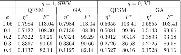
are shown in Table 1 (2) for various values ofϕ (λ) and for hyperexponential (exponen-tial) inter-arrival distribution with µ = 1.8 (η = 0.2) for Table 1 (2). From Table 1 we observe that both the optimal mean service rate in working vacation and the minimum cost decrease as ϕ increases. From Table 2 as the mean arrival rate increases both the optimal mean service rate in regular busy period and the minimum cost increase. Note that this increase in the optimal service rate withλis as expected in view of the stability of the system.
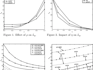
Figure 1 illustrates the influence of the traffic intensity ρ on the expected queue length for different values of VI probability,q, with η = 0.7 and exponential inter-arrival distri-bution. Here,Lq increases with ρ. From the figure one can also infer that Lq is lower for
the model with vacation interruption whenµ > η and the effect is reversed whenµ < η. Further, q has no effect on Lq when µ = η. Therefore, the condition µ > η should be
maintained in order to get better performance for the VI model.
Table 1. The optimal values η∗ and F∗ for various values ofϕ.
q= 1, SWV q= 0, VI
QFSM GA QFSM GA
ϕ η∗ F∗ η∗ F∗ η∗ F∗ η∗ F∗
0.05 0.7984 113.04 0.7984 113.04 0.5655 103.41 0.5655 103.41 0.1 0.7122 108.30 0.7139 108.30 0.5081 99.96 0.5143 99.96 0.2 0.5322 99.29 0.5324 99.29 0.3912 93.18 0.3893 93.18 0.3 0.3367 90.66 0.3364 90.66 0.2726 86.58 0.2725 86.58 0.4 0.1137 82.14 0.1125 82.14 0.1527 80.16 0.1528 80.16
Table 2. The optimal valuesµ∗ andF∗ for various values ofλ.
q= 1, SWV q= 0, VI
QFSM GA QFSM GA
λ µ∗ F∗ µ∗ F∗ µ∗ F∗ µ∗ F∗
1.2 0.2775 52.47 0.2726 52.47 0.3022 51.05 0.3093 51.06 1.4 0.3042 57.03 0.3042 57.03 0.3347 54.44 0.3356 54.44 1.6 0.3304 61.81 0.3304 61.81 0.3666 57.73 0.3764 57.75 1.8 0.3563 66.85 0.3563 66.85 0.3980 60.96 0.3979 60.96 2.0 0.3819 72.14 0.3922 72.17 0.4289 64.15 0.4288 64.15
vacationη at different q for Erlang-3 inter-arrival time distribution. As expected, Lq
de-creases with the increase of η and the larger the probability q, the larger Lq becomes.
That is the model with VI (q = 0) performs better than the model without VI (q = 1). Moreover, whenη= 0 andη=µthen clearlyq has no effect on the average queue length. Figure 3 shows the expected queue length as a function of the maximum batch size b
for different values ofϕand q with hyper-exponential inter-arrival time distribution. The figure demonstrates that the expected queue length decreases as b and ϕ increase. The decrease ofLq with the increase ofϕis due to the fact that mean vacation time decreases
and the server is available with shorter breaks. As in Figure 2, here also the larger the probabilityq, the larger Lq becomes.
Figure 4 depicts the influence of the minimum thresholdcon the expected queue length for different values of λ and q with deterministic inter-arrival distribution and b = 18. Here, Lq increases with c, λ and q. Since c is the minimum threshold to start service,
increasingcwill result in greater accumulation of customers in the queue thereby increasing
Lq. From the figure observe thatLq is lower for the model with VI for fixed λand c.
Figure 5 demonstrates the impact of the minimum batch size (a) on the expected queue length with deterministic inter-arrival distribution forc= 15 andb= 18. Here we considered four cases of the model: SWV without change over time (SWV, no CHOV), SWV with change over time (SWV, CHOV), SWV with VI and no change over time (VI, no CHOV) and SWV with VI and change over times (VI, CHOV). For all the cases consideredLq increases as aincreases. The results in the figure highlight the model with
change over time performs better and the model where both VI and change over time are introduced has best performance.
The impact ofα onLq forq = 1 andq = 0 is presented in Figures 6 and 7, respectively.
This is due to the fact that as α gets larger the mean duration of change over times becomes smaller so that the server will go for another vacation without waiting for an arrival for some reasonable duration of time. This contributes forLq to increase. It is also
observed that the system performs better for deterministic inter-arrival time distribution. Figure 8 shows the average cost as a function ofµandη for exponential inter-arrival time distribution. The figure demonstrates the existence of an optimal value (µ∗, η∗).
0.2 0.3 0.4 0.5 0.6 0.7 6
7 8 9 10 11 12 13 14
ρ Lq
q=1,SWV q=0.6 q=0,VI
0 0.1 0.2 0.3 0.4 0.5 0.6 0.7 10
15 20 25 30
η Lq
q=1,SWV 0.6 q=0,VI
Figure 1. Effect ofρ on Lq. Figure 2. Impact ofη onLq.
10 12 14 16 18 20 22 24 8
9 10 11 12 13 14 15
b
Lq
φ=0.1,q=1,SWV
φ=0.1,q=0.6
φ=0.1,q=0,VI
φ=0.2,q=1,SWV
φ=0.2,q=0.6
φ=0.2,q=0,VI
8 9 10 11 12 13 14 15 16 17 9
10 11 12 13 14 15 16 17 18
c
Lq
λ=3.5
λ=5.0
q=1,SWV
q=0.6
q=0,VI
q=1,SWV
q=0.6 q=0,VI
Figure 3. Expected queue length vsb. Figure 4. Impact ofc on Lq.
5 6 7 8 9 10 11 12
11 11.5 12 12.5 13 13.5 14
a
Lq
SWV,no CHOV SWV,CHOV VI,no CHOV VI,CHOV
0.5 1 1.5 2 2.5 3 14.9
15 15.1 15.2 15.3 15.4 15.5
α Lq
Hyperexponential Exponential Erlang−3 Deterministic
q=1,SWV
0.5 1 1.5 2 2.5 3 10.55
10.6 10.65 10.7 10.75 10.8 10.85 10.9 10.95 11 11.05
α Lq
Hyperexponential Exponential Erlang−3 Deterministic
q=0,VI
0.5 0.6
0.7 0.8
0.9 1
0.2 0.4 0.6 0.8 1 78 80 82 84 86 88 90 92 94 96
µ η
Average cost
q=0
Figure 7. Effect ofα on Lq. Figure 8. Average cost vsµand η.
From the above numerical discussion we note the following:
In terms ofLq, the model with vacation interruption performs better. Therefore to offer
a better service under the working vacation policy, one can consider vacation interruption policy that utilizes the server and decreases the queue size effectively. It also economizes the average cost.
6. Conclusion
In this paper, we have carried out an analysis of a renewal input infinite buffer batch service queue with SWV with change over time and BS-VI that has potential applications in production, manufacturing, traffic signals and telecommunication systems, etc. We have used a recursive method to obtain the steady state queue length distributions at pre-arrival and arbitrary epochs. Performance measures such as the average queue length and the average waiting time in the queue have been obtained along with a suitable cost function. The quadratic fit search method and genetic algorithm are applied to search for the optimal values of the system parameters. The method of analysis used in this paper can be applied toGIX/M(a,c,b)/1 andM AP/M(a,c,b)/1 queues with change over times and BS-VI that are left for future investigation.
Acknowledgement. The authors thank the referee of this paper for all his suggestions and corrections.
References
[1] Servi, L. D. and Finn, S. G. (2002), M/M/1 queues with working vacations (M/M/1/W V), Perf. Eval., 50, 41-52.
[2] Baba, Y. (2005), Analysis of aGI/M/1 queue with multiple working vacations, Oper. Res. Lett., 33, 201-209.
[3] Chae, K. C., Lim, D. E. and Yang, W. S. (2009), TheGI/M/1 queue and theGI/Geo/1 queue both with single working vacation, Perf. Eval., 66, 356-367.
[4] Li, J. and Tian, N. (2011), Performance analysis of a GI/M/1 queue with single working vacation, Appl. Math. Comput., 217, 4960-4971.
[5] Banik, A., Gupta, U. C. and Pathak, S. (2007), On the GI/M/1/N queue with multiple working vacations - Analytic analysis and computation, Appl. Math. Model., 31, 1701-1710.
[6] Goswami, V. and Mund, G. B. (2011), Analysis of discrete-time batch service renewal input queue with multiple working vacations, Comp. Indus. Engg., 61, 629-636.
[8] Li, J., Tian, N. and Liu, W. (2007), Discrete timeGI/Geo/1 queue with multiple working vacations, Queueing Systems, 56, 53-63.
[9] Tian, N. and Zhang, Z. G. (2006), Vacation Queueing Models: Theory and Applications, Springer, NewYork.
[10] Li, J. and Tian, N. (2007), TheM/M/1 queue with working vacations and vacation interruption, J. Sys. Sci. Sys. Engg., 16, 121-127.
[11] Li, J., Tian, N. and Ma, Z. (2008), Performance analysis ofGI/M/1 queue with working vacations and vacation interruption, Appl. Math. Model., 32, 2715-2730.
[12] Zhao, G., Du, X. and Tian, N. (2009),GI/M/1 queue with set-up period and working vacation and vacation interruption, Int. J. Infor. Manage. Sci., 20, 351-363.
[13] Jain, M., Sharma, G. C., and Sharma, R. (2011), Working vacation queue with service interruption and multi optional repair, Int. J. Infor. Manage. Sci., 22, 157-175.
[14] Zhang, M. and Hou, Z. (2011), Performance analysis ofM AP/G/1 queue with working vacations and vacation interruption, Appl. Math. Model., 35, 1551-1560.
[15] Zhang, H. and Shi, D. (2009), TheM/M/1 queue with Bernoulli-schedule-controlled vacation and vacation interruption, Int. J. Infor. Manage. Sci., 20, 579-587.
[16] Li, T., Zhang, L. and Xu, X. (2012), TheGI/Geo/1 queue with start-up period and single working vacation and Bernoulli vacation interruption, J. Infor. & Comput. Sci., 9, 2659-2673.
[17] Gao, S. and Liu, Z. (2013), AnM/G/1 queue with single working vacation and vacation interruption under Bernoulli schedule, Appl. Math. Model., 37, 1564-1579.
[18] Tadj, L., Choudhury, G. and Tadj, C. (2006), A bulk quorum queueing system with a random setup time underN- policy and with Bernoulli vacation schedule, Int. J. Prob. Stoch. Pro., 78, 1-11. [19] Baburaj, C. and Surendranath, T. M. (2005), AnM/M/1 bulk service queue under the policy (a, c, d),
Int. J. Agri. Stat. Sci., 1, 27-33.
[20] Baburaj, C. (2010), A discrete time (a, c, d) policy bulk service queue, Int. J. Infor. Manage. Sci., 21, 469-480.
[21] Haupt, R. L. and Haupt, S. E. (2004), Practical Genetic Algorithms, John Wiley and Sons, Inc., Hoboken, New Jersey, Canada.
[22] Lin, C. H. and Ke, J. C. (2010), Genetic algorithm for optimal thresholds of an infinite capacity multi-server system with triadic policy, Expert Sys. Appl., 37, 4276-4282.
[23] Lin, C. H. and Ke, J. C. (2011), Optimization analysis for an infinite capacity queueing system with multiple queue-dependent servers: genetic algorithm, Int. J. Comp. Math., 88, 1430-1442.
[24] Rao, S. S. (2009), Engineering Optimization: Theory and Practice, John Wiley & Sons, New Jersey. [25] Rardin, R. L. (1997), Optimization in Operations Research, Prentice Hall, New Jersey.
P. Vijaya Laxmiis an Assistant Professor in the Department of Applied Mathematics, Andhra University, Visakhapatnam, India. She received her M.Sc and Ph.D. degrees from Indian Institute of Technology, Kharagpur, India. Her main areas of research interest are continuous and discrete-time queueing models and their applications. She has publications in various Jour-nals like Operations Research Letters, Queueing Systems, Applied Mathe-matical Modelling, International Journal of Applied Decision Sciences, Jour-nal of Industrial and Management Optimization (JIMO), etc.
V. Goswami for a photography and short biography, see page 251.