Advanced Loop-flow Method for Fast
Hydraulic Simulations
Željko Vasilić
1, Miloš Stanić
1, Zoran Kapelan
2and Dušan Prodanović
1 1 University of Belgrade, Faculty of Civil Engineering, Serbia.2 University of Exeter, College of Engineering, Mathematics and Physical Sciences, UK. [email protected], [email protected]
Abstract
Solution of the nonlinear system of equations describing the network hydraulics problem can be formulated in several different manners, yielding various methods of solution. The most popular formulation is probably the Global Gradient Algorithm (GGA). Loop-flow formulation is another method revisited by number of researchers in recent years. Loop-flow method has the smaller system matrix to solve, which is a benefit over the GGA’s matrix, coming from the fact that real networks typically have far less loops than nodes. However, need for cumbersome pre-processing to identify network loops and sparsity of solution matrix, which is highly dependent of implemented loop identification algorithm, remain key drawbacks of existing loop-flow methods. In addition, systematic testing on the real life networks of different topologies and complexities is still somewhat lacking in the literature. In this paper, new loop-flow type method based on the novel TRIangulation BAsed Loop identification algorithm (TRIBAL) coupled with efficient implementation of loop-flow based hydraulic solver (ΔQ) is presented. Performance of the new TRIBAL ΔQ method based solver is tested through the comparison with the reference GGA solver. Preliminary results show that significant calculation speedups can be achieved with proposed method, maintaining prediction accuracy and convergence of the reference solver.
1
Introduction
The problem of water distribution system (WDS) analysis was systematized for the first time by Hardy Cross (Cross 1936). In past, many different methods and algorithms have been developed for the purpose of solving the flow and pressure distribution problem in the network, represented with the system of non-linear equations. As there are two sets of dependent unknowns (flows and pressures), selection of primary set of unknowns for which system is solved will yield different solution formulation. In most general classification of methods, they can be divided in two categories: 1) node equations based methods and 2) loop equations based methods (loop-flow methods). Solution matrix
Volume 3, 2018, Pages 2155–2161
of node based methods is larger than the one of the loop-flow methods, however the later method requires somewhat complicated pre-processing of network data (such as identification of the network loops), which can get cumbersome for networks of increased complexity. The need for such pre-processing takes away from the loop-flow methods the advantage of having the smaller solution matrix compared to the node based methods (Todini & Rossman 2013). Probably the most popular method of solution is the node based Global Gradient Algorithm (GGA) (Todini & Pilati 1987), which is adopted in the Environmental Protection Agencies’ hydraulic analysis software EPANET. In recent years researchers presented different methodologies in an attempt to further improve the WDS analysis. Many of the newly presented methods are based on modifications of GGA method due to its wide acceptance and success achieved through its implementation in the EPANET software (Simpson et al. 2014; Simpson & Elhay 2011; Deuerlein et al. 2016). On the other hand, some researchers revisited the loop-flow method to solve network hydraulics (Alvarruiz & Vidal 2015; Ivetić et al. 2016), for years being left in the shadow of the GGA’s success. As identified in aforementioned papers, loops identification procedure remains main task to deal with for the efficient implementation of the loop-flow method, as identification of the loops in any network is not unique. Consequently, identified set of loops will define the sparsity of the Jacobian solution matrix and affect the efficiency of the solver.
In this paper, new algorithm for the identification of the network loops, based on the graph theory and constrained Delaunay triangulation is presented (TRIBAL). It is coupled with more efficient implementation of the loop-flow based solver to result in new TRIBAL-ΔQ method for the hydraulic analysis of WDS. Performance of the improved loop-flow based solver implemented in TRIBAL-ΔQ method is compared against: 1) GGA’s implementation in EPANET and 2) the loop-flow based solver that uses arbitrary set of loops (ASL- ΔQ). Comparison is made in terms of computational efficiency and convergence. ASL- ΔQ solver is introduced in order to highlight the influence of identified set of loops on the computational efficiency of the loop-flow based solver.
2
Methods
2.1
Loop-flow method (ΔQ method)
ΔQ method is based on solving the head-loss equations for all loops in the network while satisfying continuity equations in all network nodes. General form of loop head-loss equation, accounting for the flow direction in the links is:
1
n
loop ij ij ij ij
ij loop ij loop
f
f
R Q Q
(1)where i and j are end nodes of a link ij, Rij is flow resistance factor, Qij is link’s flow and n is
head-loss exponent. Loop-flow correction terms (ΔQ) are introduced in the loops in arbitrarily direction and flows in the former equation are expressed as the sum of initial flows (that satisfy continuity equation) and the introduced loop-flow corrections. Equations for all loops will form the non-linear system, written in matrix form as follows:
T
T
n1
T
o o o o
where M is loops incidence matrix relating loops to links; R is the link flow resistance vector; Qo
is the links initial flow vector; ∆Q is the loops flow correction vector; Ao is the network incidence
matrix, based on initial flows direction, reduced to source nodes; Ho is the vector of fixed heads at
source nodes and operator ○ is Hadamard operator used for notation of element wise matrix operations. Number of equations in the system above (eq. 2) corresponds to the total number of loops in the network (nL). Two different types of loops can exist in any network: a) real loops formed
between the junctions of the network (in eq. 1
f
loop
0
) and b) pseudo loops formed between thesource nodes in the network (in eq. 1
f
loop
H
ij,
H
ijbeing head difference between the source nodes i and j). Number of real loops (nRL) can be expressed as nRL=Nl-Nn+1 and number of pseudoloops (nPL) as nPL=Ns-1, where Nl is the number of links, Nn number of nodes and Nsnumber of
sources (tanks and reservoirs) in the network. Linearization of the non-linear system using Newton-Raphson linearization method will yield iterative solution for the loop-flow correction vector in the following matrix form:
-1 1
i i i i
ΔQ
= ΔQ - J f
(3)where i is the iteration number and J is the iteration matrix, also known as the Jacobian matrix, containing the derivatives of the head loss functions for each loop in respect to loop flow corrections.
2.2
TRIangulation BAsed Loops identification algorithm (TRIBAL)
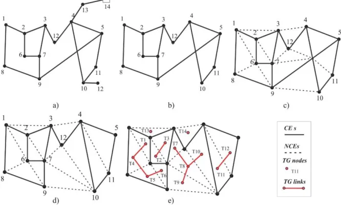
Unlike other available loops identification algorithms, that are based on the graph theory and various heuristics (Alvarruiz & Vidal 2015; Ivetić et al. 2016), the TRIBAL algorithm proposed here makes use of the graph theory and the Delaunay Triangulation (DT) algorithm. The DT algorithm is robust and efficient method, well known and proven in the field of computational geometry. For a given planar set of points, DT creates a mesh of triangles in such manner that there are no points inside of the circumcircle of any triangle created. In this research, constrained DT (CDT), which predefines some edges of triangulation is employed. The TRIBAL algorithm’s steps are listed and briefly illustrated on the following simple example (Figure 1).
Algorithm steps are: 1) Removing branched parts of the network (b); 2) Defining the set of constrained edges (CEs) for triangulation and perform CDT (c); 3) Modify the triangulation if network graph is not planar (by removing link 9-5) (d); 4) Identification of the non-constrained edges of CDT (NCEs) and creation of the triangles graph (TG) across NCEs (e); 5) Identification of outer triangle subgraphs and their deletion (T9-T8-T10-T7 and standalone T13 and T14 on Figure 1d); 6) Aggregation of remaining inner triangle subgraphs into loops (three loops); 7) Identifying loops created by the crossing links removed in the 3rd step (one loop) and 8) Identification of pseudo loops
(loops between tanks and reservoirs), which are not present in the simple example. Pseudo loops are determined via Breadth First Search (BFS) propagation algorithm from one source node to all others. The use of the BFS algorithm ensures that identified pseudo loops have minimal topological length.
2.3
TRIBAL-ΔQ method implementation
Here proposed method is implemented in two phases. TRIBAL algorithm is used as a pre-processor to identify loops (1st phase) for the follow on hydraulic simulation performed within improved ΔQ hydraulic solver (2nd phase). Hydraulic solver is implemented in the EPANET’s source code and compiled using C programing language to allow proper comparison of computational times with the reference GGA solver, already implemented in EPANET. Two new functions are added to the EPANET toolkit – ENInitLoops and ENRunLoops. ENInitLoops uses loops data obtained using the TRIBAL algorithm to allocate additional memory for the simulation purposes, while ENRunLoops performs hydraulic simulation of the network based on the improved ΔQ hydraulic solver. Various subroutines for efficient implementation of the ΔQ hydraulic solver are added in the ENRunLoops, which serves only as an interface function.
Above described implementation enables fast and reliable solution of networks’ hydraulics, which starts with the calculation of initial flow distribution. Initial flow distribution in the network is obtained using back propagation through the minimum resistance spanning tree and applying continuity equation in nodes. System of loop-flow equations is solved using the same Cholesky factorization as in EPANET. Calculation of new coefficients for the links is done using EPANET’s newcoeff routine, which calculates inverse links headloss derivatives with respect to the link flow. This is convenient as links headloss derivatives with respect to the loop-flow corrections, used in the ΔQ based hydraulic solver, are only an inverse of those coefficients calculated by the newcoeff. During the iterative calculation, update of the coefficients is done only for the links that are part of loops, since other researchers proved that this part of calculation has the most significant computational burden (Alvarruiz & Vidal 2015). Iterative calculation for the loop-flow corrections (eq.3) is done until target convergence criteria (eps) is met. Head distribution in the network is easily obtained using the spanning tree and calculated head-losses.
2.4
Case study
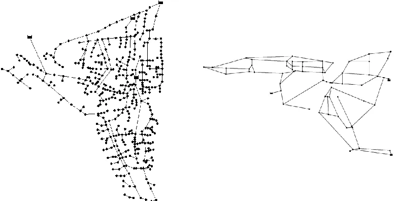
For the preliminary analysis, two benchmark networks, shown in Figure 2, are used: 1) Balerma Irrigation Network (BIN) and 2) Pescara network (PES). Characteristics of the case study networks are summarized in the Table 1. Loop factor parameter (LF) is introduced to illustrate “loop-ness” of
the network. It is calculated as the ratio of the number of links that belong to at least one loop and the total number of links. LF value ranges between 0 (branched network) and 1 (network with no branched
parts).
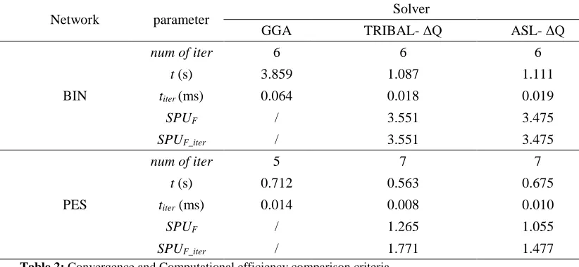
Flow and head distribution in the networks are solved using three different solvers: 1) GGA solver implemented in EPANET, 2) TRIBAL-ΔQ method solver and 3) ASL-ΔQ solver which is different than the TRIBAL-ΔQ only in the fact that it uses an arbitrary set of loops instead of the one determined with the TRIBAL algorithm. Two comparison criteria are used to compare aforementioned solvers: 1) computational efficiency (calculation speed) and 2) convergence (number of iterations). Two speedup factors are introduced as a measurement of speedup achieved with the loop-flow based solver compared to the GGA:
_
(
)
(
)
;
(
)
(
)
iter
F F iter
iter
t
GGA
t GGA
SPU
SPU
t
Q
t
Q
(4)where SPUF is speedup factor for the entire simulation and SPUF_iter is speedup factor per
iteration. Simulation times reported here are execution times for the hydraulic solvers and do not include the initialization and pre-process tasks. Reported times are determined as average time of 10 series of 10,000 cumulative algorithm runs. Target convergence criteria used is eps = 10-3.
Figure 2: Case study networks layout: BIN network (left) and PES network (right)
Network Nn Nl Ns nRL nPL nL LF
BIN 447 454 4 8 3 11 0.36
PES 71 98 3 28 2 30 0.96
Table 1: Characteristics of the case study networks
3
Results
Performance of the three used solvers are illustrated, and compared per set comparison criteria, in the Table 2. From the Table 2 it is clear that in the case of BIN network, significant speedup factor of
same number of iterations, TRIBAL-ΔQ being more efficient per iteration as the solution matrix is smaller and not all link coefficients are updated in each iteration. In the case of PES network speedup factor is much smaller (SPUF =1.265), but it is not negligible. This is expected as the loop factor for
PES network is almost 1 (LF=0.96), compared to relatively low value of loop factor for BIN network
(LF =0.36). In this case TRIBAL-ΔQ solver requires additional two iterations, when compared to the
GGA, due to the significantly different initial flow distribution and larger number of loops (than the BIN network).
As indicated in the introduction, ASL- ΔQ solver is introduced in order to highlight the influence of identified set of loops on the computational efficiency of the loop-flow based solver. When compared to the TRIBAL-ΔQ solver, ASL- ΔQ solver reaches target accuracy in the same number of iterations, but achieves lower speedup factors. The decrease of the SPUF is 2.14 % for the BIN
network and 16.61 % for the PES network. This is a consequence of reduced solution matrix sparsity of ASL- ΔQ solver compared to the TRIBAL-ΔQ solver. Solution matrix sparsity can be expressed through the number of non-zero elements in the Cholesky factor of the Jacobian matrix, shown in the Table 3. From the Table 3 it is clear that in the case of BIN network there are only two additional non-zero elements when ASL- ΔQ solver is used, compared to the TRIBAL-ΔQ solver, thus resulting in relatively small decrease in speedup factor. On the other hand, for PES network there are 51 additional non-zero elements, which influence calculation speed significantly.
Network parameter Solver
GGA TRIBAL- ΔQ ASL- ΔQ
BIN
num of iter 6 6 6
t (s) 3.859 1.087 1.111
titer (ms) 0.064 0.018 0.019
SPUF / 3.551 3.475
SPUF_iter / 3.551 3.475
PES
num of iter 5 7 7
t (s) 0.712 0.563 0.675
titer (ms) 0.014 0.008 0.010
SPUF / 1.265 1.055
SPUF_iter / 1.771 1.477
Table 2: Convergence and Computational efficiency comparison criteria
Network GGA TRIBAL- ΔQ ASL- ΔQ
BIN 1035 27 29
PES 236 90 141
Table 3: Number of non-zero elements in the Cholesky factor of the Jacobian matrix
4
Conclusion
calculation speed is a result of: 1) application of new TRIBAL algorithm for identification of optimal loops in the network, which proved to be able to identify a set of loops that will result in a highly sparse solution matrix; 2) improved ΔQ solver updating only relevant links coefficients and 3) efficient implementation of new data structures needed for loop flow method in the C source code. Speedup achieved with this method, compared to the GGA, implies that the method could be convenient for the optimization tasks where multiple hydraulic runs are necessary and topology remains unchanged (e.g. sectorization of WDS). Further investigation will be taken to account for simulations with flow control devices and pressure driven analysis purposes. Speedup achieved with this method, compared to the GGA, implies that the method could be convenient for the optimization tasks where multiple hydraulic runs are necessary (e.g. sectorization of WDS).
References
Alvarruiz, F. & Vidal, A.M., 2015. Improving the Efficiency of the Loop Method for the Simulation of Water Distribution Systems. , 141(10), pp.1–10.
Cross, H., 1936. Analysis of flow in networks of conduits or conductors. University of Illinois Bulletin: Engineering Experiment Station, (286).
Deuerlein, J.W., Elhay, S. & Simpson, A.R., 2016. Fast Graph Matrix Partitioning Algorithm for Solving the Water Distribution System Equations. Journal of Water Resources Planning and Management, 142(1). Available at: http://ascelibrary.org/doi/10.1061/%28ASCE%29WR.1943-5452.0000561.
Ivetić, D. et al., 2016. Speeding up the water distribution network design optimization using the DQ method. Journal of Hydroinformatics, 18(1), pp.33–48. Available at: http://jh.iwaponline.com/content/early/2015/10/24/hydro.2015.118.
Simpson, A. & Elhay, S., 2011. Jacobian Matrix for Solving Water Distribution System Equations with the Darcy-Weisbach Head-Loss Model. Journal of Hydraulic Engineering, 137(6), pp.696–700.
Simpson, A.R., Elhay, S. & Alexander, B., 2014. Forest-Core Partitioning Algorithm for Speeding Up Analysis of Water Distribution Systems. Journal of Water Resources Planning and Managem§ent, 140(4), pp.435–443.
Todini, E. & Pilati, S., 1987. A gradient method for the analysis of pipe network. International Conference on Computer Applications for Water Supply and Distribution, (October).