Vol. 9, No. 4, 2017 Article ID IJIM-00833, 10 pages Research Article
A New Group Data Envelopment Analysis Method for Ranking
Design Requirements in Quality Function Deployment
J. Pourmahmoud∗†, E. Babazadeh ‡
Received Date: 2015-11-02 Revised Date: 2016-04-09 Accepted Date: 2016-12-11
————————————————————————————————–
Abstract
Data envelopment analysis (DEA) is an objective method for priority determination of decision making units (DMUs) with the same multiple inputs and outputs. DEA is an efficiency estimation technique, but it can be used for solving many problems of management such as rankig of DMUs. Many re-searchers have found similarity between DEA and MCDM techniques. One of the earliest techniques in MCDM is Quality Function Deployment (QFD) which is a team-based and disciplined approach to product design, engineering and production and provides in-depth evaluation of a product. The QFD team is responsible for assessing the relationships between costumer requirements (CRs) and design requirements (DRs) and the interrelationships between DRs. In practice, each member demonstrates significantly different behavior from the others and generates different assessment results, leading to the QFD with uncertainty. In this paper data envelopment analysis is used to overcome this uncertainty. Each member’s subjective assessment is taken into account directly and a new data envelopment analysis method in group situation is constructed which differs from multi-objective decision making models. Then, without using Charnes-Cooper transformation, the proposed model is transformed into a linear programing problem in a completely different manner. We will call the proposed model ”Grouped-QFDEA”.
Keywords: Data Envelopment Analysis (DEA); Quality function deployment (QFD); Group situation; Multi-objective decision making models; Ranking.
—————————————————————————————————–
1
Introduction
D
Eproduction management literature for per-A [1] is one of the most popular tools in formance measurement, while QFD [2, 3] is one of the extremely powerful tools that is useful in product design and development and for bench-marking. The goal of DEA is to determine the∗Corresponding author.
[email protected], Tel: +989141015382
†Department of Applied Mathematics, Azarbaijan
Shahid madani University, Tabriz, Iran.
‡Department of Applied Mathematics, Azarbaijan
Shahid madani University, Tabriz, Iran.
production efficiency of DMUs by comparing how well the DMU converts inputs into outputs, while the goal of QFD is to produce a product with high quality by translating the CRs into DRs. A comprehensive literature review of QFD and its extensive applications is provided by Chan and Wu [4]. In practice, a QFD team is set up to determine the importance levels of DRs. Tra-ditionally, QFD rates the DRs with respect to CRs, and aggregates the ratings to get relative importance scores of DRs [5]. Decision makers (DMs) or design engineers usually do not have sufficient information about the influence of en-gineering responses on CRs, due to the lack of
information from the customer. These consider-ations have made the applicconsider-ations of imprecise problems in QFD. There are several studies to deal with this vague nature of QFD [6,7,8]. QFD is known by it’s house of quality (HOQ) which has a matrix format [2]. HOQ is an important tool for QFD activities, containing information on ”what”, i.e., customer requirements (CRs), ”how”, i.e., design requirements (DRs), relation-ship between ”CR” and ”DR”, and a triangular-shaped matrix placed over the design require-ments corresponds to the interrelationship be-tween them. Traditional QFD uses the weighted sum method to rank DRs [5]. There are stud-ies to determine the priority for CRs and DRs in QFD literature. The relative importance of CRs may be obtained using simple methods such as direct rating, or more complex ones such as the swing methods [9], the analytic hierarchy pro-cess (AHP) [10], a well-known and commonly used multi-criteria decision making method, and it’s variants: fuzzy AHP, analytic network pro-cess (ANP) [11] and fuzzy ANP. On the other hand, traditional QFD process dose not explic-itly incorporate cost and environmental factors. These factors are incorporated in further anal-ysis. Some studies have considered the level of difficulty, some others cost or ease of implementa-tion. However in general, studies have considered only one extra factor in their analysis [12,13]. For the first time, in 2009, Ramanathan and Yun-feng [14] applied DEA to incorporate cost and environmental factors in QFD. They proved that the relative importance values computed by data envelopment analysis (DEA) coincide with tradi-tional QFD calculations when only the ratings of DRs with respect to customer needs are consid-ered and only one additional factor, namely cost, is considered. They view each DR as a decision making unit (DMU). Using the input and output definition in DEA, they classify CRs and other factors as inputs and outputs. So CRs and fac-tors like ease of implementation are considered as outputs and factors like cost and level of difficulty as inputs. If there is no inputs (like in traditional QFD) they use a dummy input with a constant value of one for all DMUs. By solving the CCR-input oriented model for each DMU (DR) they get the relative importance of each DR. They use Assurance Region (AR) [15] in order to im-pose the weights of CRs. If there are significant
interrelationships between DRs, before applying the model, they use Wasserman [5] suggestion to normalize the relationship between DRs and CRs (and other additional factors). Kamvysi et al. [16] discussed the combination of QFD with analytic hierarchy process-analytic network pro-cess (AHP-ANP) and DEAHP-DEANP method-ologies to prioritize selection criteria in a service context. In 2013, Azadi and Farzipoor Saen [17] applied Russell measure [18] in QFD and devel-oped this model in imprecise situation. In this regards, QFD-imprecise enhanced Russell graph measure (QFD-IERGM) is proposed for incorpo-rating the criteria such as cost of services and implementation easiness in QFD. However, in general, these studies do not take into account DM’s different ideas directly in their methodolo-gies; only the model proposed by Ramanathan and Yunfeng i.e. QFD-DEA methodology, uses arithmetic average to obtain the final overall ef-ficiency scores in such uncertainty environment. In this paper, DM’s different ideas are consid-ered in a group environment and in order to deal with this situation, a group methodology based on DEA is suggested. In this regards, at first a new DEA model for ranking DRs is proposed and then will be extended to the group situation. Without using Charnes-Cooper translation, the proposed model is linearized. This proposed lin-ear programming model is applied in QFD and the uncertainty problem is overcome. In this pa-per we do not try to describe DEA and QFD tech-niques in details. Interested readers are referred to some prominent studies. The rest of this pa-per is organized as follows: QFD and the use of DEA in estimating the relative importances of DRs in QFD are explained in section 2 The pro-posed ranking method is presented in section 3. Section 4is the extension of the proposed model in group situation. Section 5 is devoted to the numerical example using proposed methodology in QFD. The final section concludes the work.
2
DEA-QFD methodology
2.1 Quality Function Deployment
QFD begins with the identification of customer requirements and their mapping into relevant engineering design requirements, as shown in Fig 1, where CR1,· · ·, CRm are the m
the n relevant engineering design requirements,
w1,· · ·, wm are the relevant importances of CRs
which wi > 0 for i = 1,· · ·, m, Rij is the
rela-tionship between CRi and DRj, and rjk is the
interrelationship betweenDRj andDRk,
satisfy-ingrjk =rkj forj, k= 1,· · ·, n.
The relationship between CRs and DRs re-flects the impact of the fulfillment of DRs on the satisfaction of CRs. These relationships should be developed by QFD team members. The relationship between CRs and DRs and the relationship between the DRs themselves are usually determined subjectively by ambiguous or vague judgments. However they are usually captured using symbols converted into crisp numbers using different measurement scales. The degree of these relationships is usually expressed on a scale system such as 0-1-3-9 or 0-1-3-5, representing linguistic expressions such as ”no relationship”, ”weak/possible relation-ship”, ”medium/moderate relationship”, and ”strong relationship”. In this paper, rating scale 0-9 is defined to characterize different strengths of the relationships between CRs and DRs as shown in Table1. Other rating scales can also be defined. It is not our purpose to explore which rating scale is the best or more appropriate for a specific situation, which is beyond the scope of this paper. As the shape of this figure looks similar to a house, so it referred to as the house of quality (HOQ). Usual procedure for
Figure 1: The house of quality in QFD
estimating the relative importances of DRs with
respect to CRs is to use weighted arithmetic aggregation rule. Note that, when there is significant interrelationships between the DRs, in many studies the following normalization procedure suggested by Wasserman [5] is usually employed for this purpose:
Rnormij =
∑n
l=1Ril·rlj
∑n j=1
∑n
l=1Ril·rlj
, ∀i, j (2.1)
where Rij denotes the relationship level in
terms of score between the CRi and DRj, and rij is the interrelationship score betweenDRi and DRj. Rijnorm is the normalized relationship value
betweenCRiandDRj, m is the number of CRs, n
is the number of DRs and∑jRnormij = 1 for each i. Thus, if there is significant interrelationships between the DRs,Rnorm
ij must be used in
estimat-ing the relative importances of DRs with respect to CRs, otherwiseRij can be directly used.
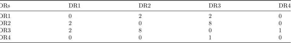
Tables 6-9 represent, respectively a determin-istic interrelationship matrix between DRs pro-vided by DMs.
2.2 Incorporating additional factors in QFD using DEA
Table 1: Rating scales for the relationships between CRs and DRs, and interrelationships between DRs themselves
Rating Definition for Relationship matrix interrelationship matrix
9 very strong relationship very strong interrelationship
7 strong relationship strong interrelationship
5 moderate relationship moderate interrelationship
3 weak relationship weakly interrelationship
1 very weak relationship very weakly interrelationship
0 no relationship no intrrelationship
2,4,6,8 the relationships between these intervals the interrelationships between these intervals
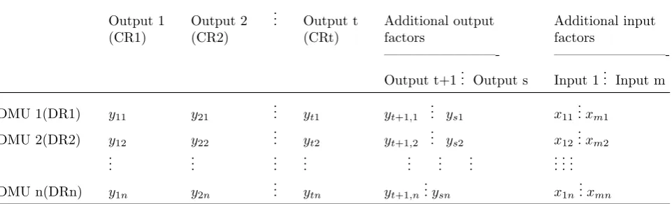
Table 2: Classification of CRs and additional factors as inputs and outputs
Output 1 Output 2 ... Output t Additional output Additional input
(CR1) (CR2) (CRt) factors factors
————————-
————————-Output t+1... Output s Input 1... Input m
DMU 1(DR1) y11 y21 ... yt1 yt+1,1 ... ys1 x11...xm1
DMU 2(DR2) y12 y22 ... yt2 yt+1,2 ... ys2 x12...xm2
..
. ... ... ... ... ... ... ... ...
DMU n(DRn) y1n y2n ... ytn yt+1,n...ysn x1n...xmn
Table 3: The relative importances of CRs
CRs CR1 CR2 CR3 CR4 CR5 CR6
The relative importance of CRs
7 10 6 5 6 6
Roll [19]. Using this logic, CRs and factors such as ease of implementation are considered as out-puts, while factors such as cost and level of diffi-culty are considered as inputs. The corresponding output-input matrices is shown in Table2.
In order to impose the relative importances of CRs, the method of Assurance region (AR) is em-ployed. Thus additional constraints that specify the relationships among the multipliers, are ap-pended to the DEA model. Hence, each DMU has m inputs and s outputs (which t of them are the CRs (t < s)), based on which the following restricted input-oriented CCR model is built to assess the efficiency score (relative importance) of DRs:
max Eo=
∑s
r=1uryro
s.t ∑mi=1vixio= 1
∑s
r=1uryrj−
∑m
i=1vixij ≤0, ∀j
ur ≥0, ∀r
vi≥0, ∀i
(2.2)
The importance of CRs is imposed, using ad-ditional constraints to form
ur=dru1; ∀r= 1,2,· · ·, t,
d1= 1
Table 4: Assessment on the relationships between the 6 CRs and 4 DRs
CRs DMs DRs
DR1 DR2 DR3 DR4
CR1 DM1 9 0 0 0
DM2 9 0 0 1
DM3 8 0 0 1
DM4 7 1 0 1
—— —— —— —— —— ——
CR2 DM1 9 1 0 0
DM2 8 1 0 0
DM3 9 1 0 0
DM4 9 1 1 0
—— —— —— —— —— ——
CR3 DM1 3 9 9 0
DM2 2 9 8 0
DM3 1 9 8 0
DM4 3 7 8 0
—— —— —— —— —— ——
CR4 DM1 0 9 9 0
DM2 0 6 9 1
DM3 0 7 9 0
DM4 1 7 9 0
—— —— —— —— —— ——
CR5 DM1 9 3 9 0
DM2 9 1 7 0
DM3 9 2 9 1
DM4 9 2 9 0
—— —— —— —— —— ——
CR6 DM1 0 0 3 9
DM2 1 1 3 9
DM3 1 1 3 9
DM4 0 1 3 9
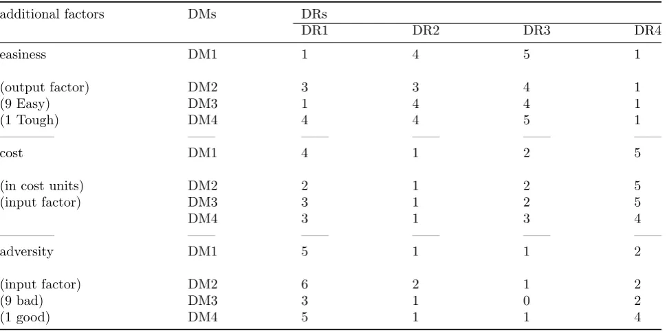
Table 5: Assessment on the relationships between the additional factors and DRs
additional factors DMs DRs
DR1 DR2 DR3 DR4
easiness DM1 1 4 5 1
(output factor) DM2 3 3 4 1
(9 Easy) DM3 1 4 4 1
(1 Tough) DM4 4 4 5 1
———— —— —— —— —— ——
cost DM1 4 1 2 5
(in cost units) DM2 2 1 2 5
(input factor) DM3 3 1 2 5
DM4 3 1 3 4
———— —— —— —— —— ——
adversity DM1 5 1 1 2
(input factor) DM2 6 2 1 2
(9 bad) DM3 3 1 0 2
Table 6: The interrelationships between DRs provided by DM1
DRs DR1 DR2 DR3 DR4
DR1 0 1 3 0
DR2 1 0 9 0
DR3 3 9 0 1
DR4 0 0 1 0
Table 7: The interrelationships between DRs provided by DM2
DRs DR1 DR2 DR3 DR4
DR1 0 2 2 0
DR2 2 0 8 0
DR3 2 8 0 1
DR4 0 0 1 0
Table 8: The interrelationships between DRs provided by DM3
DRs DR1 DR2 DR3 DR4
DR1 0 1 3 0
DR2 1 0 7 0
DR3 3 7 0 1
DR4 0 0 1 0
Table 9: The interrelationships between DRs provided by DM4
DRs DR1 DR2 DR3 DR4
DR1 0 1 3 2
DR2 1 0 9 0
DR3 3 9 0 1
DR4 2 0 1 0
Table 10: The efficiency scores of the four design requirements and their ranking order using Grouped QFDEA
DR1 DR2 DR3 DR4
E.S. 0.1475 0.0407 0.0449 0.1513
R. O. 3 1 2 4
d2 = 0.5 and d3 = 3. So, the model (2.2) can be
rewritten as follows:
max Eo=
∑s
r=1uryro s.t ∑∑mi=1vixio = 1
s
r=1uryrj−
∑m
i=1vixij ≤0, ∀j ur=dru1, r= 1,· · ·, t
ur≥0, ∀r vi≥0, ∀i
(2.3)
The linear programming model (2.3) is solved for all the DMUs to estimate their relative scores.
3
New DEA Methodology
Let there be n decision making units as DM Uj
(j= 1,2, · · ·, n), that convert m inputs xij (i=
1,2, · · ·, m) into s outputsyrj (r= 1,2, · · ·, s)
and letDM U0be a DMU under evaluation.
max θ0 =
∑s
r=1uryr0
∑m i=1vixi0
s.t. θj =
∑s
r=1uryrj
∑m i=1vixij
, ∀j
∑n
j=1θj = 1
ur≥ε, ∀r vi ≥ε, ∀i θj ≥ε, ∀j
(3.4)
Where ur(r = 1,2,· · ·, s) are the weights of
outputs, vi(r = 1,2,· · ·, m) are the weights of
inputs and θj(j = 1,2,· · ·, n) are the efficiency
score ofDM Uj. Hereεis a small amount of
pos-itive. So the last three constraints are caused that all variables ur(r = 1,2,· · ·, s), vi(r =
1,2,· · ·, m) and θj(j = 1,2,· · ·, n) are always
positive values.
Theorem 3.1 The nonlinear programming model (3.4) can be transformed to the following linear programming model:
min ∑mi=1vixi0−
∑s
r=1uryr0
s.t. ∑mi=1wijxij −
∑s
r=1uryrj = 0, ∀j
∑n
j=1wij =vi, ∀i
ur ≥ε, ∀r vi ≥ε, ∀i wij ≥ε, ∀i, j
(3.5)
Proof. From the constraints of model (3.4), it is obvious that the value of objective function is between zero and one, i.e. 0∑ ≤ θ0 ≤ 1, so 0 ≤
s
r=1uryr0
∑m i=1vixi0
≤ 1. Multiplying each part of the
inequality with−∑mi=1vixi0, and then adding the
term∑mi=1vixi0 to each part of the inequality, we
have
0≤
m
∑
i=1
vixi0− s
∑
r=1
uryr0 ≤ m
∑
i=1
vixi0.
So, the fractional objective function can be transformed to the linear objective function. Also by using the constraints of model (3.4), we can rearrange the constraints as
∑m
i=1xij(viθj)−
∑s
r=1uryrj = 0, ∀j
∑n
j=1viθj =vi ∀i.
So by using the transformation wij = viθj we
can give the model (3.5).
4
Grouped-DEA model
Letθ0(k) be the relative efficiency score ofDM U0
obtained from the model (3.5), that provided by the kth decision maker (DMk)(k = 1,2,· · ·, K)
and hk>0 be its relative importance weight
sat-isfying ∑Kk=1hk = 1. Then, we have
max ∑Kk=1hkθ (k) 0
s.t. θ(jk)= ∑s
r=1uryrj(k)
∑m i=1vix
(k) ij
, ∀j
∑K k=1
∑n j=1hkθ
(k)
j = 1
ur ≥ε, ∀r vi≥ε, ∀i θj ≥ε, ∀j.
(4.6)
The model (4.6) is equivalent with the following multi-objective programming model:
max h1
∑s
r=1ury(1)r0
∑m
i=1vix(1)i0
.. .
max hK
∑s r=1ury
(K) r0
∑m i=1vix
(K) i0
s.t. ∑mi=1wij(k)x(ijk)−∑sr=1uryrj(k)= 0, ∀j
∑k k=1
∑n j=1hkw
(k)
ij =vi, ∀i
ur≥ε, ∀r vi ≥ε, ∀i wij ≥ε, ∀i, j
(4.7)
the following linear programming model:
min {∑mi=1vix(ik0)−
∑s
r=1hkuryr(k0), ∀k}
s.t. ∑mi=1w(ijk)x(ijk)−∑sr=1ury(rjk)= 0, ∀j
∑k k=1
∑n j=1hkw
(k)
ij =vi, ∀i ur≥ε, ∀r
vi ≥ε, ∀i wij ≥ε, ∀i, j
(4.8)
Proof. From the constraints of model (4.7), it is obvious that the value of each objective function is between zero and one, i.e.
0≤hk
∑s
r=1uryr(k0)
∑m
i=1vix(i0k)
≤1.
Similar the proof of Theorem 3.1, multiplying each part of the inequality with −∑mi=1vix(i0k),
and then adding the term ∑mi=1vix(ik0) to each
part of the inequality, we have:
0≤
m
∑
i=1
vix(i0k)− s
∑
r=1
hkuryr(k0) ≤ m
∑
i=1
vix(i0k).
So, the multi-objective fractional function can be transformed to the linear objective function.
Theorem 4.2 If an optimal solution of the fol-lowing single objective programming exists, then this optimal solution will be an efficient solution of model (4.8).
min ∑Kk=1(∑mi=1vix(ik0)−
∑s
r=1hkuryr(k0)) s.t. ∑mi=1wij(k)x(ijk)−∑sr=1uryrj(k)= 0,∀j, k
∑k k=1
∑n
j=1hkw(ijk)=vi, ∀i ur ≥ε, ∀r
vi ≥ε, ∀i wij ≥ε, ∀i, j
(4.9)
Proof. Let v∗i and u∗r be an optimal solution of model (4.9). Suppose that vi∗ and u∗r is not an efficient solution of model (4.8), then there exist
vi′ andu′r such that for some k have : ∑m
i=1v∗ix (k) io −
∑s
r=1hku∗ry (k) ro >
∑m i=1v
′ ix
(k) io −
∑s r=1hku
′ ry
(k) ro
and for l∈K\khave ∑m
i=1v∗ix (l) io −
∑s
r=1hku∗ry (l) ro
∑m i=1v
′ ix
(l) io −
∑s r=1hku
′ ry
(l) ro
It follows that ∑K
k=1
∑m i=1v∗ix
(k) io −
∑K k=1
∑s
r=1hku∗ry (k) ro >
∑K k=1
∑m i=1v
′ ix
(k) io −
∑K k=1
∑s r=1hku
′ ry
(k) ro
This contradicts that v∗i and u∗r is an opti-mal solution of model (4.9).
In particular, when k=1, the LP model (4.9) is reduced to the LP model (3.5). So, model (3.5) is a special case of the LP model (4.9) for group decision making. Solving the LP model (4.9) for each DMU, we can obtain the relative efficiency of each DMU under group decision making.
5
Numerical example
In this section, we apply our approach to the information existed in the Tables 3-9. Suppose there are six CRs and four DMs. The relative importances of CRs are presented in Table 3.
Table4 represents the assessment information provided by four DMs on the relationships be-tween six CRs and four DRs. The relationships between three additional factors (cost, ease of im-plementation (easiness) and adverse environmen-tal impact (adversity)) and DRs are shown in Ta-ble 5.
6
Conclusion
The goal of QFD is producing a product with high quality. In this way ranking the DRs is so important in QFD, specially, when each member of QFD-team demonstrates different assessment from the others, leading to QFD with vague na-ture. QFD-DEA, the methodology proposed by Ramanathan, uses CCR-input oriented model to rank the DRs. This methodology uses arithmetic average to obtain the final overall efficiency scores in such uncertainty environment. In this paper, we proposed a group DEA model which gener-ates efficiency scores for each DR while consid-ering the subjective assessments of DMs in one model. It is expected that the new QFD-DEA methodology can play an important role in the studies and applications of the QFD and even, in the all team-based managements approaches. Our future research work is to extend the pro-posed methodology in Fuzzy environment. This will be researched in near future.
References
[1] A. Charnes, W. W. Cooper, A. Y. Lewin, L. M. Seiford, Data envelopment analysis : the-ory, methodology and application, Kluwer: Boston,(1994).
[2] J. R. Haruse, D. Clausing, The house of qual-ity,Harward Business Review 66 (1988) 63-73.
[3] L. Cohen, Quality Function Deployment: How to Make QFD Work for You, Addison Wesley, Reading, MA(1995).
[4] L. K. Chan, M. L. Wu, Quality function deployment: A literature review, European Journal of Operational Research 143 (2002) 463-497.
[5] G. S. Wasserman, On how to prioritize de-sign requirements during the Qfd planning process,IIE Transactions 25 (1993) 59-65. [6] Y. Chen, R. Y. K. Fung, J. Tang, Rating
technical attributes in fuzzy QFD by inte-grating fuzzy weight average method and fuzzy expected value operator, European Journal of Operational Research 174 (2006) 1553-1566.
[7] E. S. S. A. Ho, Y. J. Lai, S. I Chang, An integrated group decision-making approach to quality function deployment, IIE Trans-actions 31 (1999) 553-567.
[8] J. Wang, Fuzzy outranking approach to pri-oritize design requirements in quality func-tion deployment, International Journal of Production Research 37 (1999) 899-916. [9] Y. Park, K. J. Kim, Determination of an
op-timal set of design requirements using house of quality, Journal of Operational Manage-ment 16 (1998) 569-581.
[10] F. Y. Partovi, An analytic model for locating facilities strategically, Omega 34 (2006) 41-55.
[11] T. L. Saaty, The analytic hierarchy process: planning, Priority setting and resource allo-cation,New York: McGraw-Hill: 1980. [12] J. Bod J, R. Y. K Fung, Cost engineering
with quality function deployment, Comput-ers & Industrial Engineering 35 (1998) 587-590.
[13] J. Tang, F. Y. K Fung, B Xu, D Wang, A new approach to qualty function deploy-ment planning with finantional considera-tion, Computers & Operations Research 29 (2002) 1447-1463.
[14] R. Ramanathan, J. Yunfeng, Incorporating cost and environmental factors in quality function deployment using data envelopment analysis,Omega 37 (2009) 711-723.
[15] W. W. Cooper, L. M. Seiford, K. Tone, Data envelopment analysis: A Comprehen-sion Text with Models, Applications, Re-frences, and DEA-Solver Software, Kluwer: Boston,(2002).
[16] K. Kamvysi, K. Gotzamani, A. C. Geor-giou, A. Andronikidis, Integrating DEAHP and DEANP into the quality function de-ployment,The TQM Journal 22 (2010) 293-316.
[18] W. W. Cooper, Z. Huang, S. X. Li, B. R. Parker, J. T. Pastor, Efficiency aggregation with Enhanced Russell measures in data en-velopment analysis, Socio-Economic Plan-ning Sciences 41 (2007) 1-21.
[19] B. Golany, Y. Roll, An application procedure for DEA, Omega 17 (1989) 237-250.
[20] M. Khodabakhshi, K. Aryavash, Ranking all units in data envelopment analysis, Applied Mathematics Letters 25 (2012) 2066-2070.
Jafar Pourmahmoud is an asso-ciate professor in Department of Applied Mathematics, Azarbai-jan Shahid madani University. He has published papers in different journals such as Journal of the Operational Research Society (JORS), Interna-tional Journal of Industrial Mathematics, Mea-surement, Applied Mathematics and computa-tion, Journal of Applied Environmental and Bio-logical Sciences, and International Journal of In-dustrial Engineering Computations and . His research interest is on Operations Research (spe-cially on Network Data Envelopment Analysis and fuzzy DEA) and Numerical Linear Algebra and Applications.