ARCH-COMP19 Category Report: Continuous and Hybrid Systems with Linear Continuous Dynamics

(1)

Volume 61, 2019, Pages 14–40

ARCH19. 6th International Workshop on Applied Verification of Continuous and Hybrid Systems

ARCH-COMP19 Category Report:

Continuous and Hybrid Systems with

Linear Continuous Dynamics

Matthias Althoff

1

_{, Stanley Bak}

2

_{, Marcelo Forets}

3

_{, Goran Frehse}

4

_{, Niklas}

Kochdumper

1

_{, Rajarshi Ray}

5

_{, Christian Schilling}

6

_{, and Stefan Schupp}

7

1 _{Technische Universit¨}_{at M¨}_{unchen, Department of Informatics, Munich, Germany} [email protected]

2 _{Safe Sky Analytics, Manlius, NY, United States} [email protected]

3 _{UTEC Universidad Tecnol´}_{ogica, Uruguay} [email protected] 4

ENSTA ParisTech, Palaiseau, France

[email protected] 5

National Institute of Technology Meghalaya, Shillong, India.

[email protected] 6

IST Austria, Klosterneuburg, Austria

[email protected] 7

RWTH Aachen University, Theory of hybrid systems, Aachen, Germany

[email protected]

Abstract

(2)

1 Introduction

Disclaimer The presented report of the ARCH friendly competition forcontinuous and hybrid systems with linear continuous dynamics aims at providing a landscape of the cur-rent capabilities of verification tools. We would like to stress that each tool has unique strengths—not all of the specificities can be highlighted within a single report. To reach a consensus in what benchmarks are used, some compromises had to be made so that some tools may benefit more from the presented choice than others. The obtained results have been verified by an independent repeatability evaluation. To establish further trustworthi-ness of the results, the code with which the results have been obtained is publicly available atgitlab.com/goranf/ARCH-COMP.

This report summarizes results obtained in the 2019 friendly competition of the ARCH workshop1 _{for verifying hybrid systems with linear continuous dynamics}

˙

x(t) =Ax(t) +Bu(t),

where A ∈ Rn×n, x∈ Rn, B ∈ Rn×m, and u∈ Rm. Participating tools are summarized in

Sec.2. The results of our selected benchmark problems are shown in Sec. 3 and are obtained on the tool developers’ own machines. Thus, one has to factor in the computational power of the processors used, summarized in AppendixA, as well as the efficiency of the programming language of the tools.

The goal of the friendly competition is not to rank the results, but rather to present the landscape of existing solutions in a breadth that is not possible with scientific publications in classical venues. Such publications would typically require the presentation of novel techniques, while this report showcases the current state-of-the-art tools. For all results reported by each participant, we have run an independent repeatability evaluation. A novelty compared to last year is that tool developers provide Dockerfiles [13] so that executing tools on one’s own machine has become much easier.

The selection of the benchmarks has been conducted within the forum of the ARCH website (cps-vo.org/group/ARCH), which is visible for registered users and registration is open for anybody. All tools presented in this report use some form of reachability analysis. This, however, is not a constraint set by the organizers of the friendly competition. We hope to encourage further tool developers to showcase their results in future editions.

2 Participating Tools

The tools participating in the categoryContinuous and Hybrid Systems with Linear Continuous Dynamics are introduced subsequently in alphabetical order.

CORA The toolCOntinuous Reachability Analyzer (CORA) [1,3,4] realizes techniques for reachability analysis with a special focus on developing scalable solutions for verifying hybrid systems with nonlinear continuous dynamics and/or nonlinear differential-algebraic equations. A further focus is on considering uncertain parameters and system inputs. Due to the modular

(3)

design of CORA, much functionality can be used for other purposes that require resource-efficient representations of multi-dimensional sets and operations on them. CORA is imple-mented as an object-oriented MATLAB code. The modular design of CORA makes it possible to use the capabilities of the various set representations for other purposes besides reachability analysis. CORA is available atcora.in.tum.de.

CORA/SX CORA/SX is a port of the basic zonotope reachability algorithm from the CORA MATLAB toolbox to SpaceEx. It varies slightly in that some matrix computations (which approximate the input over one time step) use SpaceEx code instead of an over-approximation that is based on intervals.

HyDRA The Hybrid systems Dynamic Reachability Analysis (HyDRA) tool implements flow-pipe construction based reachability analysis for linear hybrid automata. The tool is built on top of HyPro [26] available atths.rwth-aachen.de/research/projects/hypro/, a C++ library for reachability analysis. HyPro provides different implementations of set representations tai-lored for reachability analysis such as boxes, convex polyhedra, support functions, or zono-topes, all sharing a common interface. This interface allows one to easily exchange the utilized set representation in HyDRA. We use this to extend state-of-the art reachability analysis by CEGAR-like parameter refinement loops, which (among other parameters) allow us to vary the used set representation. Furthermore, HyDRA incorporates the capability to explore different branches of the search tree in parallel. Being in an early state of development, HyDRA already shows promising results on some benchmarks, although there is still room for improvements. An official first release is planned.

Hylaa The tool Hylaa [9,10] computes the reachable set using discrete-time semantics. Hylaa is a Python-based tool, which can produce live plots during computation, as well as images and video files of the reachable set. Hylaa’s website ishttp://stanleybak.com/hylaa.

(4)

JuliaReach JuliaReach is a toolbox for reachability computations of dynamical systems [14], available athttp://juliareach.org. It is written in Julia, a modern high-level language for scientific computing. Compared to last year, JuliaReach now has support for hybrid systems (and also nonlinear dynamics). The continuous-time reachability algorithm for linear systems uses a block decomposition technique based on support functions presented in [15]. This tech-nique partitions the state space, projects the initial states to subspaces, and propagates these low-dimensional sets in time. This allows us to perform otherwise expensive set operations in low dimensions. Furthermore, if the output does not depend on all dimensions, we can effectively skip the reach set computation for the respective dimensions. For checking safety properties in purely continuous time, we only compute the reachable states symbolically, which allows us to make the minimal number of support-function evaluations. JuliaReach also offers an option to analyze systems with discrete-time semantics as in Hylaa. For the set computa-tions we use the LazySets library, which is also part of the JuliaReach toolbox. For some of the models we use our custom SX parser for parsing SX (SpaceEx format) model files, and otherwise we create the models manually in Julia. For next year we plan to extend the toolbox with complementary techniques and algorithms to make it more effective, which is now easy with our new architecture.

SpaceEx SpaceEx is a tool for computing reachability of hybrid systems with complex, high-dimensional dynamics [20,21,19]. It can handle hybrid automata whose continuous and jump dynamics are piecewise affine with nondeterministic inputs. Nondeterministic inputs are par-ticularly useful for modeling the approximation error when nonlinear systems are brought to piecewise affine form. SpaceEx comes with a web-based graphical user interface and a graphical model editor. Its input language facilitates the construction of complex models from automata components that can be combined to networks and parameterized to construct new components. The analysis engine of SpaceEx combines explicit set representations (polyhedra), implicit set representations (support functions) and linear programming to achieve a maximum of scala-bility while maintaining high accuracy. It constructs an overapproximation of the reachable states in the form of template polyhedra. Template polyhedra are polyhedra whose faces are oriented according to a user-provided set of directions (template directions). A cover of the continuous trajectories is obtained by time-discretization with an adaptive time-step algorithm. The algorithm ensures that the approximation error in each template direction remains below a given value. SpaceEx is available athttp://spaceex.imag.fr.

(5)

3 Verification of Benchmarks

For the 2019 edition, we have decided to keep all benchmarks from our 2018 friendly competition [2], but solve them with our updated tools. In addition, we have modified the Spacecraft Rendezvous benchmark and the Gearbox benchmark. In the Spacecraft Rendezvous benchmark we have increased the uncertainty of the time of the switch to the passive (abort) mode, which can be significantly more challenging to verify. Regarding the Gearbox benchmark, we have added an instance with a larger initial set.

Special Features We briefly list the special features of each benchmark:

• Space station benchmark from [27]: This is a purely continuous benchmark with 270 state variables and three inputs. This year, it is the benchmark with the largest amount of continuous state variables.

• Spacecraft Rendezvous benchmark from [16]: This benchmark has hybrid dynamics and is a linearization of a benchmark in the other ARCH-COMP category Continuous and Hybrid Systems with Nonlinear Dynamics. Consequently, the reader can observe the difference in computation time and verification results between the linearized version and the original dynamics.

• Powertrain benchmark from [5, Sec. 6]: This is a hybrid system for which one can select the number of continuous state variables and the size of the initial set. Up to 51 continuous state variables are considered.

• Building benchmark from [27, No. 2]: A purely continuous linear system with a medium number of continuous state variables; the benchmark does not only have safety properties, but also ones that should be violated to check whether the reachable sets contain certain states.

• Platooning benchmark from [12]: A rather small number of continuous state variables is considered, but one can arbitrarily switch between two discrete states: a normal operation mode and a communication-failure mode.

• Gearbox benchmark from [17]: This benchmark has the smallest number of continuous state variables, but the reachable set does not converge to a steady state and the reachable set for one point in time might intersect multiple guards at once.

Types of Inputs Generally, we distinguish between three types of inputs:

1. Fixed inputs, where u(t) is precisely known. If in addition, u(t) = const, the linear system becomes an affine system ˙x(t) =Ax(t) +b. For instance, the gearbox benchmark has affine dynamics.

2. Uncertain but constant inputs, where u(t) ∈ U ⊂ Rm is uncertain within a set U, but

each uncertain input is constant over time: u(t) =const.

3. Uncertain, time-varying inputs u(t)∈ U ⊂_Rm _where _u₍_t₎ ₆₌_const_{. Those systems do}

(6)

Different Paths to Success When tools use a fundamentally different way of solving a benchmark problem, we add further explanations.

Computation Time The computation times specified in this report include the computation time of the reachable set and the time needed for the verification of the specifications.

3.1 International Space Station Benchmark

3.1.1 Model

The International Space Station (ISS) is a continuous linear time-invariant system ˙x(t) =

Ax(t) +Bu(t) proposed as a benchmark in ARCH 2016 [27]. In particular, the considered system is a structural model of component 1R (Russian service module), which has 270 state variables with three inputs.

The specification deals with the possible range for outputy3, which is a linear combination

of the state variables (y = Cx, C ∈ _R3×270_). _{Initially all 270 variables are in the range}

[−0.0001,0.0001], u1 is in [0,0.1],u2 is in [0.8,1], andu3 is in [0.9,1]. The time bound is 20.

Discrete-time analysis for the space station benchmark should be done with a step size of 0.01. The A, B, and C matrices are available in MATLAB format2 (that can also be opened with Python using scipy.io.loadmat) and in SpaceEx format3. There are two versions of this benchmark:

ISSF01 The inputs can change arbitrarily over time: ∀t:u(t)∈ U.

ISSC01 (constant inputs) The inputs are uncertain only in their initial value, and constant over time: u(0)∈ U, ˙u(t) = 0.

3.1.2 Specifications

The verification goal is to check the ranges reachable by the output y3, which is a linear

combination of the state variables. In addition to the safety specification, for each version there is an UNSAT instance that serves as sanity checks to ensure that the model and the tool work as intended. But there is a caveat: In principle, verifying an UNSAT instance only makes sense formally if a witness is provided (counter-example, under-approximation, etc.). Since most of the participating tools do not have this capability, we run the tools with the same accuracy settings on an SAT-UNSAT pair of instances. The SAT instance demonstrates that the over-approximation is not too coarse, and the UNSAT instance demonstrates that the over-approximation is indeed conservative, at least in the narrow sense of the specification.

ISS01 Bounded time, safe property: For allt∈[0,20],y3(t)∈[−0.0007,0.0007]. This property

is used with the uncertain input case (ISSF01) and assumed to be satisfied.

ISS02 Bounded time, safe property: For allt∈[0,20],y3(t)∈[−0.0005,0.0005]. This property

is used with the constant input case (ISSC01) and assumed to be satisfied.

ISU01 Bounded time, unsafe property: For all t ∈ [0,20], y3(t) ∈ [−0.0005,0.0005]. This

property is used with the uncertain input case (ISSF01) and assumed to be unsatisfied.

ISU02 Bounded time, unsafe property: For all t ∈ [0,20], y3(t) ∈ [−0.00017,0.00017]. This

property is used with the constant input case (ISSC01) and assumed to be unsatisfied.

2_{slicot.org/objects/software/shared/bench-data/iss.zip}

(7)

3.1.3 Results

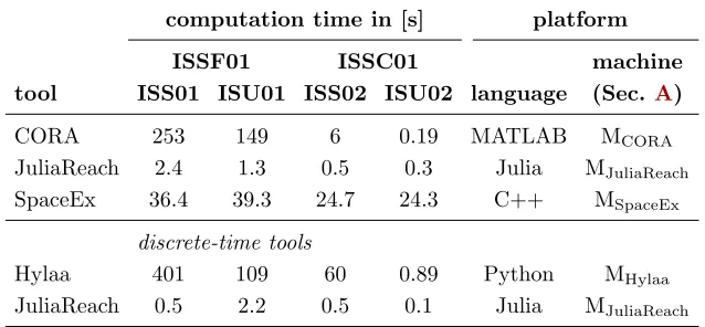
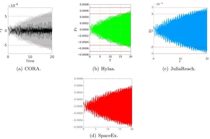
Results of the international space station benchmark for statey3over time are shown in Fig.1

and Fig.2. The computation times of various tools for the benchmark are listed in Tab.1.

Note CORA CORA was run with a step size of 0.01 and with a zonotope order of 30 for benchmark version ISSF01. For version ISSC01 a step size of 0.02 and a zonotope order of 10 was used.

Note JuliaReach We used the following step sizes (in dense time): 0.0006 for ISSF01 and 0.005 for ISSC01. Moreover, we handled inputs in a wrapping-free way. The matrix exponential obtained from the discretization is very sparse, which we can exploit in our decomposition-based approach. For the property we need to compute (symbolic) reachable states for 135 variables. We used a two-block partition with each block consisting of 135 variables.

Note SpaceEx SpaceEx was run with the LGG scenario. The sampling was chosen as 0.005 for ISSF01 and 0.05 for ISSC01. The template directions were taken to be±y3, so only two

directions. Sincey3 is an algebraic variable that is a linear expression of the state variables,

we replaced it in the forbidden states and the direction definition by the corresponding linear expression. To model the constant inputs in ISSC01, we introducedu1, u2, u3as state variables

with ˙u1= ˙u2= ˙u3= 0. A custom algorithm for constant inputs could avoid such an artificial

augmentation and significantly reduce the runtime for ISSC01. Note that SpaceEx treats the initial states as a general polyhedron, i.e., a linear program is solved at every time step. SpaceEx also computes the full matrix exponential, a 270×270 matrix, even though in the LGG algorithm it would suffice to compute the vectoreAt`for each template direction`.

Since SpaceEx does not currently support the plotting of algebraic variables, we used the following trick to plot y3 over time: we introduced a state variable z with dynamics ˙z =

−1000(z−y3). Since the time constant forz is about two orders of magnitude below that of

y3, we expect the plots to practically identical to a true plot ofy3.

Table 1: Computation Times for the International Space Station Benchmark

computation time in [s] platform

ISSF01 ISSC01 machine

tool ISS01 ISU01 ISS02 ISU02 language (Sec.A)

CORA 253 149 6 0.19 MATLAB MCORA

JuliaReach 2.4 1.3 0.5 0.3 Julia MJuliaReach

SpaceEx 36.4 39.3 24.7 24.3 C++ MSpaceEx

discrete-time tools

Hylaa 401 109 60 0.89 Python MHylaa

(8)

(a) CORA. (b) Hylaa. (c) JuliaReach.

(d) SpaceEx.

Figure 1: ISS: Reachable sets ofy3 plotted over time for the uncertain input case.

(d) SpaceEx.

(9)

3.2 Spacecraft Rendezvous Benchmark

3.2.1 Model

Spacecraft rendezvous is a perfect use case for formal verification of hybrid systems since mis-sion failure can cost lives and is extremely expensive. This benchmark is taken from [16]; its original continuous dynamics is nonlinear, and the original system is verified in the ARCH-COMP categoryContinuous and Hybrid Systems with Nonlinear Dynamics. When spacecraft are in close proximity (such as rendezvous operations), a common approximation to analyze the nonlinear dynamics is to use the linearized Clohessy-Wiltshire-Hill (CWH) equations [18]. This benchmark analyzes this linear hybrid model.

The hybrid nature of this benchmark originates from a switched controller, while the dy-namics of the spacecraft is purely continuous. In particular, the modes areapproaching (100m-1000m), rendezvous attempt (less than 100m), and aborting. Discrete-time analysis for the rendezvous system should be done with a step size of 0.1. The model is available in C2E2, SDVTool, and SpaceEx format on the ARCH website4. The set of initial states is

X0=

    −900 −400 0 0     ⊕    

[−25,25] [−25,25]

0 0     .

In previous years, there were two versions of this benchmark:

SRNA01 The spacecraft approaches the target as planned and there exists no transition into theaborting mode.

SRA01 A transition intoaborting mode occurs at timet= 120 [min].

This year, we have added additional instances that transition to theabortingmode at different times, in order to increase the analysis difficulty and add unsafe cases. This required increasing the analysis time horizon to 300 minutes. The additional instances are as follows.

SRA02 A transition intoaborting mode occurs nondeterministically,t∈[120,125] [min].

SRA04 A transition intoaborting mode occurs at timet= 240 [min].

An initial, discrete-time analysis indicated it is safe to enter theabortingmode up to around timet= 250 [min]. We also added the following two instances, which are presumably unsafe. For timing, tools should use the same settings for these as for the safe cases.

SRU01 A transition intoaborting mode occurs at timet= 260 [min].

SRU02 A transition intoaborting mode occurs nondeterministically,t∈[0,260] [min].

(10)

Given the thrust constraints of the specified model, in moderendezvous attempt, the absolute velocity must stay below 0.055 m/s. In the aborting mode, the vehicle must avoid the target, which is modeled as a boxBwith 0.2 m edge length and the center placed as the origin. In the rendezvous attempt the spacecraft must remain within the line-of-sight coneL={[x, y]T |(x≥ −100m)∧(y≥xtan(30◦₎₎_∧₍₋_y_≥_x_tan(30◦₎₎_}_{. It is sufficient to check these parameters for}

a time horizon of 300 minutes.

Let us denote the discrete state by z(t) and the continuous state vector by x(t) = [sx, sy, vx, vy]T, where sx and sy are the positions in x- and y-direction, respectively, and vx

andvy are the velocities in x- and y-direction, respectively. The mode approaching is denoted

byz1, the moderendezvous attempt byz2, and the modeabortingbyz3. We can formalize the

specification as

SR02 ∀t∈[0,300min],∀x(0)∈ X0: (z(t) =z2) =⇒

q

v2

x+vy2≤0.055m/s∧

[sx, sy]T ∈ L

∧(z(t) =z3) =⇒ ([sx, sy]T ∈ B/ ).

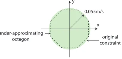
To solve the above specification, all tools under-approximate the nonlinear constraint

q

v2

x+v2y≤0.055m/sby an octagon as shown in Fig.3.

x y

0.055m/s

under-approximating

octagon original

constraint

Figure 3: Under-approximation of the nonlinear velocity constraint by an octagon.

Remark on nonlinear constraint In the original benchmark, the constraint on the ve-locity was set to 0.05 m/s, but it can be shown that this constraint cannot be satisfied by a counterexample. For this reason, we have relaxed the constraint to 0.055 m/s.

3.2.3 Results

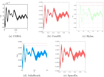
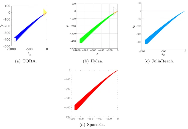
Results of the spacecraft rendezvous benchmark for thesx-sy-plane are shown in Fig.4for the

version SRNA01 and in Fig.5for the version SRA01. The computation times of various tools for the spacecraft rendezvous benchmark are listed in Tab.2.

(11)

In order to find suitable orthogonal directions for the method in [22], we perform the following procedure: first, we project the last zonotope not intersecting the guard set onto the guard set; second, we apply principal component analysis to the generators of the projected zonotope, providing us with the orthogonal directions.

Note Hylaa Hylaa was run with urgent (0-step) transitions disabled, since upon entering the approaching mode, the state may be on the boundary of the line-of-sight cone (strict inequalities are not allowed by linear programming tools and therefore not allowed in Hylaa either).

Note HyDRA We used a time step of 0.1 and support functions with octagonal templates. The time horizon was set to 300.

Note JuliaReach We used a step size (in dense time) of 0.04 and a one-block partition. The flowpipe was overapproximated with hyperrectangles. We handled discrete transitions by computing the intersection with invariants and guards lazily before overapproximating with a hyperrectangle.

Note SpaceEx SpaceEx was run with the LGG scenario, box directions, and a flowpipe tolerance of 0.2.

(d) SpaceEx.

Figure 4: Reachable sets for the spacecraft rendezvous benchmark in thesx-sy-plane for the

(12)

(a) CORA. (b) Hylaa.

-500 -400 -300 -200 -100 0 100

-1000 -800 -600 -400 -200 0 200

(c) HyDRA.

(d) JuliaReach. (e) SpaceEx.

Figure 5: Reachable sets for the spacecraft rendezvous benchmark in thesx-sy-plane for the

benchmark variant with maneuver abortion att= 120 [min] (SRA01, over analysis time horizon of 300 [min])

Table 2: Computation Time [s] for the Spacecraft Rendezvous Benchmarks (SR*) for Specifi-cationSR02.

tool NA01 A01 A02 A03 A04 A05 A06 A07 A08 U01 U02

CORA 4.7 1.4 1.2 1.7 3.6 3.7 3.7 7.8 28.5 8.3 30.6

HyDRA – 0.73 – – – – – – – – –

JuliaReach 1.0 1.3 – – – – – – – 1.8 1.7

SpaceEx 0.33 0.31 – – – – – – – 0.48 2.6

discrete-time tools

Hylaa 9.0 2.3 2.8 15 30 48 53 15 180 26 489

(13)

3.3 Powertrain with Backlash

3.3.1 Model

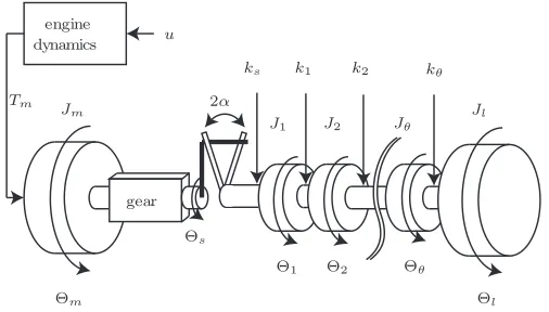
The powertrain benchmark is an extensible benchmark for hybrid systems with linear continu-ous dynamics taken from [5, Sec. 6] and [8, Sec. 4]. The essence of this benchmark is recalled here, and the reader is referred to the above-cited papers for more details. The benchmark considers the powertrain of a vehicle consisting of its motor and several rotating masses repre-senting different components of the powertrain, e.g., gears, differential, clutch, among others, as illustrated in Fig.6. The benchmark is extensible in the sense that the number of continuous states can be easily extended ton= 7+2θ, whereθis the number of additional rotating masses. The number of discrete modes, however, is fixed and originates from backlash, which is caused by a physical gap between two components that are normally touching, such as gears. When the rotating components switch direction, for a short time they temporarily disconnect, and the system is said to be in the dead zone. The model is available in SpaceEx format on the ARCH website5. Discrete-time analysis for the powertrain system should be done with a step size of 0.0005 (5.0E-4).

The set of initial states is

X0={c+αg|α∈[−1,1]},

c= [−0.0432,−11,0,30,0,30,360,−0.0013,30, . . . ,−0.0013,30]T, g= [0.0056,4.67,0,10,0,10,120,0.0006,10, . . . ,0.0006,10]T.

Jm

J1 J2 Jθ

Jl

ks k1 k2 kθ

Θm

Θ1 Θ2 Θθ

Θl gear

engine

dynamics u

Tm

Θs 2α

Figure 6: Powertrain model.

We analyze an extreme maneuver from an assumed maximum negative acceleration that lasts for 0.2 [s], followed by a maximum positive acceleration that lasts for 1.8 [s]. The initial states of the model are on a line segment in then-dimensional space. We create different difficulty levels of the reachability problem by scaling down the initial states by some percentage. The

(14)

model has the following non-formal specification: after the change of direction of acceleration, the powertrain completely passes the dead zone before being able to transmit torque again. Due to oscillations in the torque transmission, the powertrain should not re-enter the dead zone of the backlash.

To formalize the specification using linear time logic (LTL), let us introduce the following discrete states:

• z1: left contact zone

• z2: dead zone

• z3: right contact zone

For all instances, the common specification is: For all t ∈[0,2],x(0) ∈ X0, (z2U z3) =⇒

G(z3). The instances only differ in the size of the system and the initial set, wherecenter(·)

returns the volumetric center of a set.

DTN01 θ= 2, X0:= 0.05(X0−center(X0)) +center(X0).

DTN02 θ= 2, X0:= 0.3(X0−center(X0)) +center(X0).

DTN03 θ= 2, no change ofX0.

DTN04 θ= 22,X0:= 0.05(X0−center(X0)) +center(X0).

DTN05 θ= 22,X0:= 0.3(X0−center(X0)) +center(X0).

DTN06 θ= 22, no change ofX0.

3.3.3 Results

Results of the powertrain benchmark in thex1-x3-plane are shown in Fig.7. The computation

times of various tools for the powertrain benchmark are listed in Tab.3.

Note CORA For all benchmark versions CORA was run with a zonotope order of 20 and with a step size of 0.0005s. The intersections with the guard sets are calculated with the mapping based approach from [5] which avoids the geometric computation of the intersection and therefore scales well with respect to the number of system states.

Note Hylaa Hylaa was run with aggregation turned off. Convex hull aggregation worked, but was slower. The current deaggregation approach in Hylaa did not work well, as overapprox-imation error seemed to allow states to remain in the dead zone indefinitely, so deaggregation was never triggered.

3.4 Building Benchmark

3.4.1 Model

This benchmark is quite straightforward: The system is described by ˙x(t) = Ax(t) +Bu(t),

u(t)∈ U,y(t) =Cx(t), whereA,B,Care provided on the ARCH website6. The initial set and the uncertain input U are provided in [27, Tab. 2.2]. Discrete-time analysis for the building system should use a step size of 0.01. There are two versions of this benchmark:

(15)

(a) CORA (DTN03). (b) Hylaa (DTN03). (c) CORA (DTN05).

Figure 7: Reachable sets in thex1-x3-plane.

Table 3: Computation Times for the Powertrain Benchmark

machine tool DTN01 DTN02 DTN03 DTN04 DTN05 DTN06 language (Sec. A)

CORA 3.26 3.17 3.31 17.8 17.9 18.3 MATLAB MCORA

discrete-time tools

Hylaa 6.45 15.2 49.6 12.6 43.2 154 Python MHylaa

BLDF01 The inputs can change arbitrarily over time: ∀t:u(t)∈ U.

BLDC01 (constant inputs) The inputs are uncertain only in their initial value, and constant over time: u(0) ∈ U, ˙u(t) = 0. The purpose of this model instance is to accommodate tools that cannot handle time-varying inputs.

The verification goal is to check whether the displacementy1of the top floor of the building

re-mains below a given bound. In addition to the safety specification from the original benchmark, there are two UNSAT instances that serve as sanity checks to ensure that the model and the tool work as intended. But there is a caveat: In principle, verifying an UNSAT instance only makes sense formally if a witness is provided (counter-example, under-approximation, etc.). Since most of the participating tools do not have this capability, we run the tools with the same accuracy settings on an SAT-UNSAT pair of instances. The SAT instance demonstrates that the over-approximation is not too coarse, and the UNSAT instance indicates that the over-approximation is indeed conservative.

BDS01 Bounded time, safe property: For all t ∈[0,20], y1(t) ≤5.1·10−3. This property is

assumed to be satisfied.

BDU01 Bounded time, unsafe property: For all t ∈ [0,20], y1(t) ≤ 4·10−3. This property

(16)

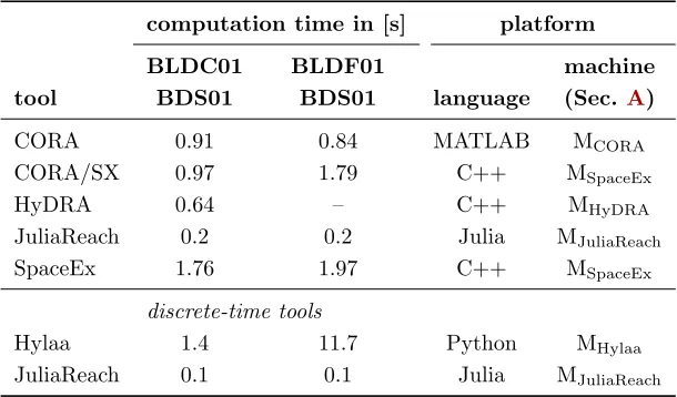
Table 4: Computation Times for the Building Benchmark

BLDC01 BLDF01 machine

tool BDS01 BDS01 language (Sec.A)

CORA 0.91 0.84 MATLAB MCORA

CORA/SX 0.97 1.79 C++ MSpaceEx

HyDRA 0.64 – C++ MHyDRA

JuliaReach 0.2 0.2 Julia MJuliaReach

SpaceEx 1.76 1.97 C++ MSpaceEx

discrete-time tools

Hylaa 1.4 11.7 Python MHylaa

JuliaReach 0.1 0.1 Julia MJuliaReach

BDU02 Bounded time, unsafe property: The forbidden states are{y1(t)≤ −0.78·10−3∧t= 20}.

This property is assumed to be violated for BLDF01 and satisfied for BLDC01. Property BDU02 serves as a sanity check to confirm that time-varying inputs are taken into account. A tool should be run with the same accuracy settings on BLDF01-BDU02 and BLDC01-BDU02, returning UNSAT on the former and SAT on the latter.

3.4.3 Results

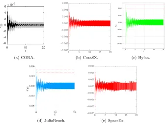
Results of the building benchmark for statex25over time are shown in Fig.8-11. The

compu-tation times of various tools for the building benchmark are listed in Tab.4.

Note CORA Since the dynamics of this example is dominated by the input after one second, we use the step size 0.002 fort∈[0,1] and the step size 0.01 fort∈[1,20]. The zonotope order is chosen as 100.

Note HyDRA We use a step size of 0.004 and support functions with an octagonal template as a state set representation.

Note JuliaReach We used the following step sizes (in dense time): 0.003 for BLDF01 and 0.005 for BLDC01. For the property we need to compute (symbolic) reachable states for only a single variable (x25). We used a three-block partition so thatx25is in its own block (the other

two blocks containx1–x24 resp. x26–x48). Furthermore, we decomposed the discretized initial

states lazily to achieve higher precision.

(17)

0 0.5 1 t

-6 -4 -2 0 2 4 6

x25

10-3

(a) CORA. (b) CoraSX. (c) Hylaa.

Figure 8: Building (BLDF01): Reachable sets ofx25plotted over time up to time 1. Some tools

additionally show possible trajectories.

3.5 Platooning Benchmark

3.5.1 Model

The platooning benchmark considers a platoon of three vehicles following each other. This benchmark considers loss of communication between vehicles. The initial discrete state isqc.

Three scenarios are considered for the loss of communication:

PLAA01 (arbitrary loss) The loss of communication can occur at any time, see Fig.12(a). This includes the possibility of no communication at all.

PLADxy (loss at deterministic times) The loss of communication occurs at fixed points in time, which are determined by clock constraints c1 andc2 in Fig. 12(b). The clockt is reset

when communication is lost and when it is re-established. Note that the transitions have must-semantics, i.e., they take place as soon as possible.

PLAD01: c1=c2= 5.

PLANxy (loss at nondeterministic times) The loss of communication occurs at any time

t ∈ [tb, tc] in Fig. 12(c). The clock t is reset when communication is lost and when it

is re-established. Communication is reestablished at any time t ∈ [0, tr]. This scenario

covers loss of communication after an arbitrarily long timet≥tc by reestablishing

com-munication in zero time.

(18)

0 10 20 t

-6 -4 -2 0 2 4 6

x25

10-3

(a) CORA. (b) CoraSX. (c) Hylaa.

Figure 9: Building (BLDF01): Reachable sets ofx25 plotted over time up to time 20. Some

tools additionally show possible trajectories.

The models are available in SpaceEx, KeYmaera, and MATLAB/Simulink format on the ARCH website7. Discrete-time analysis for the platoon system should use a step size of 0.1.

Discussion The arbitrary-loss scenario (PLAA) subsumes the other two instances (PLAD, PLAN).

The verification goal is to check whether the minimum distance between vehicles is preserved. The choice of the coordinate system is such that the minimum distance is a negative value.

BNDxy Bounded time (no explicit bound on the number of transitions): For allt∈[0,20] [s],

x1(t)≥ −dmin [m],x4(t)≥ −dmin [m],x7(t)≥ −dmin[m], where dmin=xy [m].

BND50: dmin= 50.

BND42: dmin= 42.

BND30: dmin= 30.

UNBxy Unbounded time and unbounded switching: For all t ≥ 0 [s], x1(t) ≥ −dmin [m],

x4(t)≥ −dmin [m],x7(t)≥ −dmin [m], wheredmin=xy [m].

UNB50: dmin = 50.

(19)

0 0.5 1 t

-8 -6 -4 -2 0 2 4 6

x25 10-3

(a) CORA. (b) CoraSX.

-0.006 -0.004 -0.002 0 0.002 0.004 0.006

0 0.2 0.4 0.6 0.8 1

(c) HyDRA.

(d) Hylaa. (e) JuliaReach. (f) SpaceEx.

Figure 10: Building (BLDC01): Reachable sets ofx25 plotted over time up to time 1. Some

UNB42: dmin = 42.

UNB30: dmin = 30.

3.5.3 Results

Results of the platoon benchmark for statex1 over time are shown in Fig.13-15. The

compu-tation times of various tools for the platoon benchmark are listed in Tab.5.

Note CORA CORA was run with zonotope order 400 and time step size 0.02 for benchmark version (PLAA01-BND50), with zonotope order 800 and time step size 0.009 for benchmark version (PLAA01-BND42), with zonotope order 20 and time step size 0.02s for benchmark version (PLAD01-BND42), and with zonotope order 200 and time step size 0.02 for benchmark version (PLAD01-BND30). For the unbounded case (PLAN01-UNB50), the reachable set at

t= 50 is increased by 1% and it is checked when this set is re-entered. Further, zonotope order 400 and time step size 0.01 are used.

For PLAA01, we use the CORA library to rewrite the hybrid automaton as a purely contin-uous system with uncertain parameters for analysis. This idea is also known ascontinuization [6,7]. After introducing the uncertain matrix

A={αAc+ (1−αAn)|α∈[0,1]}

we can abstract the model in Fig.12(a)by

˙

(20)

0 10 20 t -8 -6 -4 -2 0 2 4 6 x25 10-3

(a) CORA. (b) CoraSX.

-0.006 -0.004 -0.002 0 0.002 0.004 0.006

0 5 10 15 20

(c) HyDRA.

(d) Hylaa. (e) JuliaReach. (f) SpaceEx.

Figure 11: Building (BLDC01): Reachable sets ofx25 plotted over time up to time 20. Some

qc

˙

x=Acx+_BcaL

x∈Dc

qn

˙

x=Anx+_BnaL

x∈Dn

(a) Arbitrary switching.

qc

˙

x=Acx+_BcaL

˙

t= 1

x∈Dc

qn

˙

x=Anx+_BnaL

˙

t= 1

x∈Dn

t=c1

t:= 0

t=c2

t:= 0

(b) Deterministic switching.

qc

˙

x=Acx+_BcaL

˙

t= 1

x∈Dc

qn

˙

x=Anx+_BnaL

˙

t= 1

x∈Dn

t∈[_{tb, tc}]

t:= 0

t∈[0, tr]

t:= 0

(c) Nondeterministic switching.

Figure 12: Three options adapted from the original benchmark proposal [12]. On the left, the system can switch arbitrarily between the modes. In the middle, mode switches are only possible at given points in time. On the right, mode switches are only possible during given time intervals.

where⊕denotes the Minkowski addition and ˜U =BcU (Bc=Bn).

(21)

Note JuliaReach We used the following step sizes (in dense time): 0.01 for PLAD01-BND42, 10−5for PLAD01-BND30, and 0.03 for PLAN01-UNB50. In all cases we used a one-block parti-tion and overapproximated the flowpipe with hyperrectangles. We handled discrete transiparti-tions by computing the intersection with invariants lazily before overapproximating with a hyperrect-angle. In the unbounded-time scenario (PLAD01), termination requires to detect a fixpoint; we check for fixpoints after every discrete transition.

(a) CORA.

Figure 13: PLAA01: Reachable sets ofx1plotted over time. CORA additionally shows possible

trajectories.

Table 5: Computation Times for the Platoon Benchmark

PLAA01 PLAA01 PLAD01 PLAD01 PLAN01 machine

tool BND50 BND42 BND42 BND30 UNB50 language (Sec.A)

CORA 4.17 13.7 0.12 0.33 85.4 MATLAB MCORA

HyDRA – – 3.2 3.45 – C++ MHyDRA

JuliaReach – – 0.6 – 9.2 Julia MJuliaReach

SpaceEx – – 0.63 9.6 159.2 C++ MSpaceEx

XSpeed – – 0.57 6.23 29.41 C++ MXSpeed

discrete-time tools

Hylaa – – 0.97 0.97 – Python MHylaa

(22)

(a) CORA (BND30).

-30 -25 -20 -15 -10 -5 0 5

0 5 10 15 20

(b) HyDRA (BND30). (c) Hylaa (BND30).

(d) JuliaReach (BND42). (e) SpaceEx (BND30). (f) XSpeed (BND30).

Figure 14: PLAD01: Reachable sets of x1 plotted over time. Some tools additionally show

possible trajectories.

3.6 Gearbox Benchmark

3.6.1 Model

The gearbox benchmark models the motion of two meshing gears. When the gears collide, an elastic impact takes place. As soon as the gears are close enough, the gear is consideredmeshed. The model includes a monitor state that checks whether the gears are meshed or free and is available in SpaceEx format8 and as a Simulink model9. Once the monitor reaches the state meshed, it stays there indefinitely.

With four continuous state variables, the gearbox benchmark has a relatively low number of continuous state variables. The challenging aspect of this benchmark is that the solution heavily depends on the initial state as already pointed out in [17]. For some initial continuous states, the target region is reached without any discrete transition, while for other initial states, several discrete transitions are required.

In the original benchmark, the position uncertainty in the direction of the velocity vector of the gear teeth (x-direction) is across the full width of the gear spline. Uncertainties of the position and velocity in y-direction, which is perpendicular to the x-direction, are considered to be smaller. Due to the sensitivity with respect to the initial set, we consider smaller initial sets. The full uncertainty in x-direction could be considered by splitting the uncertainty in x-direction and aggregating the individual results. For discrete-time analysis of the gearbox system, a step size of 0.0001 (1.0E-4) should be used.

8_{cps-vo.org/node/34375}

(23)

(a) CORA (UNB50). (b) JuliaReach (UNB50). (c) SpaceEx (UNB50).

(d) XSpeed (UNB50).

Figure 15: PLAN01: Reachable sets ofx1 plotted over time.

GRBX01: The initial set isX0= 0×0×[−0.0168,−0.0166]×[0.0029,0.0031]×0.

GRBX02: The initial set isX0= 0×0×[−0.01675,−0.01665]×[0.00285,0.00315]×0.

3.6.2 Specification

The goal is to show that the gears aremeshed within a time frame of 0.2 [s] and that the bound

x5≤20 [Nm] of the cumulated impulse is met. Using the monitor statesfreeandmeshed, and a

global clockt, this can be expressed as a safety property as follows: For allt≥0.2, the monitor should be inmeshed. Under nonblocking assumptions, this means that t <0.2 whenever the monitor is not inmeshed, i.e., when it is infree.

MES01: forbidden states: (free∧t≥0.2)∨(x5≥20)

3.6.3 Results

Results of the benchmark for statex3 andx4 are shown in Fig.16. The computation times of

various tools for the benchmark are listed in Tab.6.

(24)

Note Hylaa Hylaa used resets to project the system state exactly onto the guard when transitioning from thefree mode.

(a) CORA. (b) Hylaa.

(c) SpaceEx.

Figure 16: Gearbox (GRBX01): Reachable sets of x3 and x4. Some tools additionally show

possible trajectories.

Table 6: Computation Times of the Gearbox Benchmark

tool GRBX01-MES01 GRBX02-MES01 language machine (Sec. A)

CORA 0.36 0.48 MATLAB MCORA

SpaceEx 0.07 0.08 C++ MSpaceEx

discrete-time tools

(25)

4 Conclusion and Outlook

This report presents the results on the third friendly competition for the formal verification of continuous and hybrid systems with linear continuous dynamics as part of the ARCH’19 workshop. The reports of other categories can be found in the proceedings and on the ARCH website: cps-vo.org/group/ARCH.

A major observation of the results is that participating tools have significantly reduced computation times compared to the previous year. Also, Dockerfiles are now available for all tools from gitlab.com/goranf/ARCH-COMP so that running the examples on one’s own machine is much easier now. Information about the competition in 2020 will be announced on the ARCH website.

5 Acknowledgments

The authors gratefully acknowledge financial support by the European Commission project UnCoVerCPS under grant number 643921, and by DST-SERB, Government of India, under grant number YSS/2014/000623.

A

Specification of Used Machines

A.1 M

CORA

• Processor: Intel Core i7-7820HQ CPU @ 2.90GHz x 4

• Memory: 32 GB

• Average CPU Mark onwww.cpubenchmark.net: 9409 (full), 2027 (single thread)

A.2 M

HyDRA

• Processor: Intel Core i7-4790K CPU @ 4.00GHz x 8

• Memory: 16 GB

A.3 M

Hylaa

• Processor: Intel Core i5-5300U @ 2.30GHz x 4

• Memory: 16 GB

A.4 M

JuliaReach

• Processor: Intel Core i5-5200 CPU @ 2.20GHz x 4

• Memory: 8 GB

(26)

A.5 M

SpaceEx

• Processor: Intel Core i9-8950HK CPU @ 2.9 GHz

• Memory: 16 GB

A.6 M

XSpeed

• Processor: Intel Xeon E5-1650 v4 @ 3.60GHz x 6

• Memory: 64 GB

References

[1] M. Althoff. An introduction to CORA 2015. InProc. of the Workshop on Applied Verification for

Continuous and Hybrid Systems, pages 120–151, 2015.

[2] M. Althoff, S. Bak, D. Cattaruzza, X. Chen, G. Frehse, R. Ray, and S. Schupp. ARCH-COMP17 category report: Continuous and hybrid systems with linear continuous dynamics. InProc. of the

4th International Workshop on Applied Verification for Continuous and Hybrid Systems, pages

143–159, 2017.

[3] M. Althoff and D. Grebenyuk. Implementation of interval arithmetic in CORA 2016. InProc.

of the 3rd International Workshop on Applied Verification for Continuous and Hybrid Systems,

pages 91–105, 2016.

[4] M. Althoff, D. Grebenyuk, and N. Kochdumper. Implementation of Taylor models in CORA 2018. In Proc. of the 5th International Workshop on Applied Verification for Continuous and

Hybrid Systems, pages 145–173, 2018.

[5] M. Althoff and B. H. Krogh. Avoiding geometric intersection operations in reachability analysis of hybrid systems. InHybrid Systems: Computation and Control, pages 45–54, 2012.

[6] M. Althoff, C. Le Guernic, and B. H. Krogh. Reachable set computation for uncertain time-varying linear systems. InHybrid Systems: Computation and Control, pages 93–102, 2011.

[7] M. Althoff, A. Rajhans, B. H. Krogh, S. Yaldiz, X. Li, and L. Pileggi. Formal verification of phase-locked loops using reachability analysis and continuization. Communications of the ACM, 56(10):97–104, 2013.

[8] S. Bak, S. Bogomolov, and M. Althoff. Time-triggered conversion of guards for reachability analysis of hybrid automata. In Proc. of the 15th International Conference on Formal Modelling and

Analysis of Timed Systems, pages 133–150, 2017.

[9] S. Bak and P. S. Duggirala. Hylaa: A tool for computing simulation-equivalent reachability for lin-ear systems. InProceedings of the 20th International Conference on Hybrid Systems: Computation

and Control, pages 173–178. ACM, 2017.

[10] S. Bak and P. S. Duggirala. Rigorous simulation-based analysis of linear hybrid systems. In

International Conference on Tools and Algorithms for the Construction and Analysis of Systems,

pages 555–572. Springer, 2017.

[11] S. Bak and P. S. Duggirala. Simulation-equivalent reachability of large linear systems with inputs.

InInternational Conference on Computer Aided Verification, pages 401–420. Springer, 2017.

[12] I. Ben Makhlouf and S. Kowalewski. Networked cooperative platoon of vehicles for testing methods and verification tools. InProc. of ARCH14-15. 1st and 2nd International Workshop on Applied

(27)

[13] Carl Boettiger. An introduction to Docker for reproducible research. ACM SIGOPS Operating

Systems Review, 49(1):71–79, 2015.

[14] S. Bogomolov, M. Forets, G. Frehse, K. Potomkin, and C. Schilling. JuliaReach: a toolbox for set-based reachability. InHSCC, 2019.

[15] S. Bogomolov, M. Forets, G. Frehse, F. Viry, A. Podelski, and C. Schilling. Reach set approxima-tion through decomposiapproxima-tion with low-dimensional sets and high-dimensional matrices. InHSCC, pages 41–50, 2018.

[16] N. Chan and S. Mitra. Verifying safety of an autonomous spacecraft rendezvous mission. InProc.

of the 4th International Workshop on Applied Verification of Continuous and Hybrid Systems,

pages 20–32, 2017.

[17] H. Chen, S. Mitra, and G. Tian. Motor-transmission drive system: a benchmark example for safety verification. InProc. of ARCH14-15. 1st and 2nd International Workshop on Applied veRification

for Continuous and Hybrid Systems, pages 9–18, 2015.

[18] WH Clohessy. Terminal guidance system for satellite rendezvous. Journal of the Aerospace

Sci-ences, 27(9):653–658, 1960.

[19] G. Frehse. Reachability of hybrid systems in space-time. In Alain Girault and Nan Guan, editors,

Proc. Int. Conf. Embedded Software, EMSOFT, Amsterdam, Netherlands, October 4-9, 2015, pages

41–50. IEEE, 2015.

[20] G. Frehse, C. Le Guernic, A. Donz´e, S. Cotton, R. Ray, O. Lebeltel, R. Ripado, A. Girard, T. Dang, and O. Maler. SpaceEx: Scalable verification of hybrid systems. InProc. of the 23rd International

Conference on Computer Aided Verification, LNCS 6806, pages 379–395. Springer, 2011.

[21] G. Frehse, R. Kateja, and C. Le Guernic. Flowpipe approximation and clustering in space-time. In C. Belta and F. Ivancic, editors, Proc. Int. Conf. Hybrid systems: computation and control,

HSCC, April 8-11, 2013, Philadelphia, PA, USA, pages 203–212. ACM, 2013.

[22] A. Girard and C. Le Guernic. Zonotope/hyperplane intersection for hybrid systems reachability analysis. In Proc. of Hybrid Systems: Computation and Control, LNCS 4981, pages 215–228. Springer, 2008.

[23] A. Gurung, A. Deka, E. Bartocci, S. Bogomolov, R. Grosu, and R. Ray. Parallel reachability analysis for hybrid systems. In ACM/IEEE International Conference on Formal Methods and

Models for System Design, MEMOCODE, pages 12–22. IEEE, 2016.

[24] R. Ray and A. Gurung. Poster: Parallel state space exploration of linear systems with inputs using xspeed. InProc. of HSCC’15, pages 285–286. ACM, 2015.

[25] R. Ray, A. Gurung, B. Das, E. Bartocci, S. Bogomolov, and R. Grosu. XSpeed: Accelerating reachability analysis on multi-core processors. InProc. of HVC 2015, volume 9434 ofLNCS, pages 3–18, 2015.

[26] S. Schupp, E. Abraham, I. Ben Makhlouf, and S. Kowalewski. HyPro: A C++ library for state set representations for hybrid systems reachability analysis. InProc. NFM’17, volume 10227 of LNCS, pages 288–294. Springer, 2017.

[27] H.-D. Tran, L. V. Nguyen, and T. T. Johnson. Large-scale linear systems from order-reduction. In Proc. of ARCH16. 3rd International Workshop on Applied Verification for Continuous and Hybrid