Vol. 45, No. 2, Fall 2013, pp. 1- 9 )AIJ-EEE)
٭
Corresponding Author, Email: [email protected]
Fast Finite Element Method Using Multi-Step Mesh
Process
M. Badiei Khuzani
1and Gh. Moradi
2٭1- PhD. Student, School of Engineering and Applied Sciences, Harvard University, Cambridge, United State 2- AssociateProfessor, Department of Electrical Engineering, Amirkabir University of Technology, Tehran, Iran
ABSTRACT
This paper introduces a new method for accelerating current sluggish FEM and improving memory
demand in FEM problems with high node resolution or bulky structures. Like most of the numerical
methods, FEM results to a matrix equation which normally has huge dimension. Breaking the main matrix
equation into several smaller size matrices, the solving procedure can be accelerated. For implementing this
matter, the meshing process should be changed. Here, a multi-step meshing process is proposed which
consists of both posterior and main levels. The posterior level is used for separating matrix equations from
each other and the main level for field computation in the problem.
The proposed approach is compatible with other optimizing method for increasing speed in FEM.
Therefore, combining this method with other methods creates a powerful asset for solving complex FEM
problems. The results show that the proposed method speeds up FEM and decreases the memory capacity. In
addition, it brings the facility of parallel computation which is of great importance in fast computational
algorithm.
KEYWORDS
1. INTRODUCTION
Finite element method as one of the most popular methods in solving boundary condition problems is usually used in electromagnetics. Laplace equation is one of the boundary value problems that use finite element method to find the distribution of electromagnetic quantities. But, one difficulty in using it as well as employing other numerical methods in electromagnetic is that they basically result in a matrix with great dimension. This usually occurs in bulky structures, where for example there are a large number of nodes, covering the body of structure to form the finite elements. So, the need of huge computation makes it necessary to use an efficient way to decrease the time of process.
Common optimizing methods, for example Wavelet transform, concentrate just on matrix equation and optimizing the solution [1]. Clearly, a deficiency about these optimization methods is that their efficiency is correlated with the matrix characteristic. For example, when the sparseness of matrix decreases, these methods fail to increase speed or the error becomes intolerable. Adaptive mesh refinement is another popular optimizing method which needs error estimators as a complementary part. This necessity limits their performance, because error estimators implicate additional computing complexity which is not desired [2-4].
In contrast to the above-mentioned methods, the proposed multi-step mesh process reduces the memory and time complexity by breaking the computing task into several parts. It shows great speed and memory improving regardless of matrix characteristics and it does not need to any kind of error estimators. In addition, it can be used with other optimizing methods. This is very great advantage over them since they are to some extent isolated from each other.
The paper continues with the optimization method in the next section, and then the meshing process and proposed method is explained. In section four, the results are compared with those of the existing methods to show the achievements of the current research. The parallel computation is studied in section 5. Finally, the paper finishes with a brief conclusion.
2. METHOD OF OPTIMIZATION
Mostly, all of the numerical methods result in a matrix form as below:
[K] [V] = [U] (1)
in which [V] is the unknown vector, [K] is the coefficient matrix and [U] is the excitation vector. Now, assume that after applying the boundary conditions, [K] be an N×N matrix, [V] and [U] be an N×1. In finite element method, the dimensions of the matrix equation depend directly to the number of nodes which is adapted for problem. So, if the number of nodes is increased to cover the whole of structure, especially in a huge structure, the complexity of matrix equation is increased. In the proposed approach, it is intended to break this large dimensional matrix
equation into a number of low dimensional matrix equations. Suppose the matrix equation is broken into M matrix equations without changing the number of nodes. The matrix equation becomes as below:
(2)
After taking care of the boundary values in our problem, each of these equations has dimension of
̅ , with ∑ ̅ . Liu and Jiao [5] showed that the memory and time complexity of solving (1) is respectively in the order of O(N ) and O(N . Clearly, if the solving process is spitted as in (2), a better performance is achieved. This is because in this case, the memory needs is in the order of
(∑ ̅ ̅ ) and the time complexity is in the order of ∑ ̅ ̅ ). To break (1) into (2), some changes in the sampling process of the function should be introduced. As will be seen in the next section, these changes prevent us to decrease as required to decrease the complexity unboundedly.
3. METHOD OF MESHING PROCESS
A. PRINCIPLES
In FEM, usually uniform polygons such as equilateral or triangle are used to cover whole the structure. In modern methods, these polygons are not uniform, and their sizes change in the regions where more precision is necessary. In this way, the amount of nodes that should be used for covering the body of structure decreases effectively. Both of these methods are depicted in figure 1. In our proposed approach, at first the domain Ω is spitted into several sub domains Ωi. For simplicity, the domain is bisected as shown in figure 2. If the nomenclature is used for the nodes on the splitter, two matrix equations is obtained which are dependent to each other through the dividing nodes as following:
[
̂ ̂ ̂ ̅ ̅
̂ ̂ ̂ ̅ ̅ ̂ ̅ ̅ ̂ ̅ ̅ ̅ ̅ ]
[
̅
̅ ]
[ ̂
̂̅ ̂ ̅̅̅̅
̂ ̅ ̅ ]
(4)
If it is desired to attain two separate matrix equations, first obtain the values. This means that the boundary values around each of these sub-domains should be determined. The key element is using a posterior level before our original mesh process as in figure 2.b.
(a)
(b)
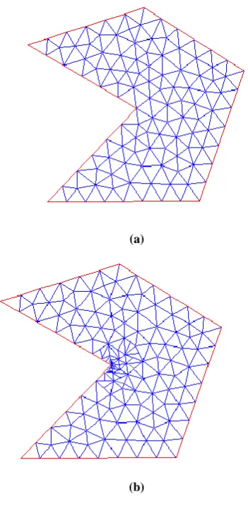
Fig. 1. (a) The traditional mesh distribution, (b) Adaptive mesh refinement.
(a)
(b)
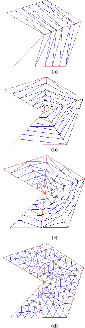
Fig. 2. (a) Dividing the shape into two parts, with splitter nodes (hollow bullets), (b) Posterior process.
In this posterior level, the triangles are built with two criteria:
1.Two nodes should be placed on the divider and another should be placed on the shape borders.
2.The triangles should cover whole the shape like the normal mesh process in FEM.
Assume ̅ to be the number of nodes on the splitter, and similarly, ̅ and ̅ be the number of nodes on the two interior nodes next to the splitter. Since ̅ ̅
̅ as a consequence of this posterior level, the complexity cannot be reduced monolithically with increasing the divisions.
Critical point here is achieving to nodes values at these posterior levels as exact as possible to avoid catastrophic error which is distributed through the main stream of steps. This issue is reviewed in section 4. After this novel sampling, the matrix equation in (4) turns to the three matrix equations in (5).
[
̅ ̅
̅ ̅ ̅ ][
̅ ] [
̅ ]
[
̅ ̅
̅ ̅ ̅ ][
̅ ] [
[
̅ ̅
̅ ̅ ̅ ][ ̅ ] [
̅ ]
It is seen that the matrix equations in (5) are independent and in the form of (2) with M=3. Consequently, the desired goal in breaking a large dimensional matrix equation into several low dimensional ones is achieved.
B DIFFERENT APPROACHES
In this section two different ways of behaving the proposed method is referred. As will be seen, each way has its own specification. A shape can be divided in two manners:
1.Sequential separation 2.Concurrent separation
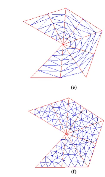
The difference between these separation styles is in their posterior process. In sequential separation, the posterior process breaks itself to several levels. So, in each level, some low dimensional matrix equations are solved. These equations increase, if the divisions are increased, but their dimensions remain under control. In contrast, in concurrent separation, there is just one pre-step level, but the dimension for its matrix equation expands by increasing the number of divisions. These states are shown in figure 3 for our previous example with eight sections.
Now, suppose there are N nodes, including interior and on-splitter nodes. The structure is divided to Q parts. Suppose { ̅ ̅ ̅ } { ̅ ̅ ̅ } show groups whose members are the amounts of interior and on-splitter nodes in respect. Hence, the number of matrix equation and related dimension are shown in table (1).
TABLE 1. NUMBER OF EQUATIONS AND MATRIX DIMENSION IN THE POSTERIOR LEVEL AND MESH PROCESS
An important point is that the adaptive mesh refinement is a special case of concurrent separation when the sub-domains increase. In adaptive mesh
refinement the domain breaks to very large number of sub-domains with using regular finite element as in figure 1. a. Each mesh is a sub-domain. After this step, each sub-domain becomes refiner with using error estimators (h-method), if necessary. In contrast, we focus on sequential separation and will survey its performance via an example in section four.
(a)
(b)
(c)
(d)
Type Method
Sequential Separation
Concurrent Separation
Po
st
er
io
r
le
v
el
Number of
equations Q-1 1
Maximum
Dimensions Max (̅ ) ∑ ̅
M
esh
p
ro
ce
ss
Number of equations Q Q
Maximum Dimensions
Max (̅) Max (̅)
(2)
(7)
(12)
(e)
(f)
Fig. 3. (a-d) Sequential separation (e-f) Concurrent separation.
C. MATHEMATICAL REVIEW OFTHE
PROCESS
In this section, the process is surveyed from mathematical point of view. Our problem is referred to the following general equation [6]:
(6)
An equivalent form of (5) is the variational or weak formulation as following:
(7)
in which V is the Sobolev space and is defined as following:
{ } (8)
We also define the following operators:
∫
∫ ∫
(9)
In the Ritz-Galerkin approximation [9], V is replaced by a subspace With this approximation, variational form turns to the following formula:
(10)
Usually, S is a piecewise polynomial space i.e. we can find a set { } that has two conditions:
1-Spans S (Be a basis for S)
2-Its members be the linear polynomials
Therefore, if , then the potential can be expressed as:
∑
(11)
in which is the nodal value, defined at each node. In regular FEM, at first the domain is partitioned, and then each basis is defined on the specific element e,g, the basis function { } is defined on the eth element. This basis is zero outside this element. In normal FEM, these partitions are solid. It means that when they are chosen, they remain unchanged during the whole process. In contrast, adaptive mesh process uses one dynamic partition that changes if it is required to give a refiner resolution at critical points. In the proposed method, several different partitions are used that are different from each other through resolution. This brings the facility to divide the task of computation of through several steps. So the memory problem is solved which is the bottle-neck of this numerical method. In the next section, this method is employed through an example.
4. IMPLEMENTATION AND RESULTS
In this section the effectiveness of the proposed method in comparison with normal FEM is studied. An example is solved with analytical solution to follow the error analysis of our method. This example is a simple electrostatic problem which is depicted in figure 4. It is a box with Dirichlet boundary condition at each face. The analytical solution for this special problem is as following [7-8]:
∑
(12)
Without loss of generality, V0 is assumed to be 7
Volts. Using this closed form equation, the potential distribution is calculated which is illustrated in figure 5. For this specific problem multi step mesh process is depicted in figures 6 and 7, distribution of each part is depicted. Clearly, total distribution has very little difference with the exact potential distribution. Figure 8 shows the numerical result from normal FEM method for the same number of nodes as multi step mesh process. Clearly, there is a little difference between two distributions. Error for both methods is plotted in figure 9. The following definition is used for the error computation:
|
|
(13)
(5)
(9)
It is seen that the convergence of our method through figure 9b-1 and figure 9b-2. Except some ripples on splitting region (y=0.5), the error plot is the same for both methods. To have a quantitative criterion for overall error, the sum of square of errors at all mesh points is calculated as:
∑ ∑
|
|
. (14)For the posterior level, this value is 1.24 times of the normal FEM. However for the final stage, it is reduced to about that of the traditional FEM. As mentioned previously, for suppressing error in splitting regions, higher dimensional polynomial (p-method) can be used for posteriori levels to obtain splitter-nodes’ values as exact as possible. By using high dimensional polynomial, the accuracy in splitting region is increased while reducing the speed because we should solve high dimensional posterior matrix in (4). Therefore, the error minimization depend on how much reduce the speed of the method is reduced.
x
y
0
V
V
0
V
0
V
0
V
w
h
Fig. 4. Dirichlet boundary condition imposed on a box.
Fig. 5. Exact distribution of Dirichlet boundary condition.
(a)
(b)
Fig. 6. Sequential multi-step mesh process with one prior level for the same problem (a) Posterior level (b) Main level.
(a) 1
(b)
Fig. 7. Distribution of potential after first priority level and splitting the shape into two parts. (a) section (2)
distribution (b) section (3) distribution.
Fig. 8. Distribution of potential with the same number of nodes, using normal FEM method.
(a)
(b-1)
(b-2)
The complexity and memory demand for each method in the above example is shown as a variable of number of nodes in figure 10. In low density of nodes, two methods have the same performance, but when node’s density increases, breaking the structure show its efficiency.
(a)
(b)
Fig. 10. Comparison between two methods in box example for one Posterior level (a) Memory complexity (b) Time Complexity.
5. PARALLEL COMPUTATION AND TIME SAVING
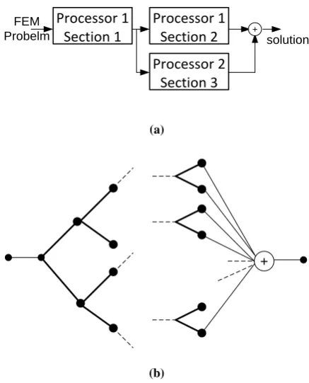
Up to this point, the time necessary for creating mesh network at each posterior level and creating new matrix for each of these levels was ignored. In general, some loops in our programming language are needed to do these jobs which reduce speed. But the most brilliant achievement of the proposed method is the facility of parallel computation which brings the speed in rendering program and solves the mentioned difficulty. In parallel computation, each parts of program can be calculated by separate processors, and then recombined to result the final solution. In figure 6, a very simple state of this situation is shown. Figure 10.a shows our previous example that can be computed in the parallel form. This
parallel computation includes creating mesh network and solving independent matrix equations as in (4). In general, this situation can be extended as it is shown in figure 10-b. Figure 11 shows the speed performance comparison, between parallel computing program and non-parallel one in the state of using two processors for previous example. Clearly, it is seen that a great speed advantage will result if the multi-step mesh method is combined with multi-processor programming.
Processor 1
Section 1
Processor 1
Section 2
Processor 2
Section 3
+
FEM
Probelm solution
(a)
+
(b)
Fig. 11. (a) Parallel computation for one posteriori level and two processors (b). Extending the situation with m-processor.
6. CONCLUSION
In this paper, a new method has been proposed to accelerate the finite element method, based on the multi-level mesh process. Clearly, the results show that the memory demand can be effectively reduced for computer analysis. This method is compatible with adaptive mesh process; therefore the both methods can be combined to use the advantages of them, simultaneously. This issue makes it very strong algorithm for the purpose of fast computation. It is anticipated that in the near future, the computer program packs adopt this method to use its features for fast analysis.
REFERENCES
[1] Yee Hui Lee and Yilong Lu, “Accelerating Numerical Electromagnetic Code Computation By Using the Wavelet transform”, IEEE Trans on MTT, vol. 34, no. 5, 1998.
[2] Thomas Grätsch, Klaus-Jürgen Bathe, “A Posteriori Error Estimation Techniques in Practical Finite Element analysis”, Elsevier, Computer and structure, 2004.
[3] Babu ̌ka I, Chandra J, Flaherty J.E. “Adaptive Computational Methods for Partial Differential Equations”, Society for Industrial and Applied Mathematics, Philadelphia, 1983.
[4] Babu ̌ka I, Zienkiewicz O.C, Gago J, Oliveira E.R, “Accuracy Estimates and Adaptive Refinements in Finite Element Computation”, New York: John Wiley and Sons, 1986
[5] Haixin Liu and Dan Jiao, “A Direct Finite-Element-Based Solver of Significantly Reduced Complexity for Solving Large-Scale Electromagnetic Problems,” Microwave Symposium Digest. MTT '09. IEEE MTT-S, pp. 177, 2009.
[6] Susanne C. Brenner and L. Ridgway Scott, “The Mathematical Theory of Finite Element Methods”, 2nd edition. New York: Springer-Verlag, 2002, pp. 1-3.
[7] Ainsworth M, Oden J.T, “A Posterior Error Estimation in Finite Element Analysis”, New York: John Wiley and Sons, 2000.
[8] Anastasis C. Polycarpou, “Introduction to the Finite Element Method in Electromagnetics”, 1st edition. California Morgan &.Claypool Publishers’ series, 2006, pp. 93-94.
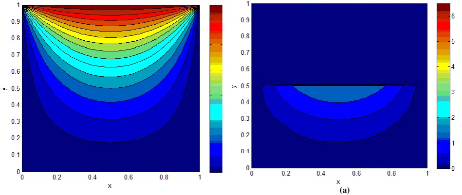
![Fig. 9. Error plot, based on absolute difference between exact values and numerical values (a) Normal FEM (b-1) proposed method’s error in Posterior level [figure 6-a], (b-2) Final stage error [Fig](https://thumb-us.123doks.com/thumbv2/123dok_us/18254.2001896/7.595.321.532.53.710/absolute-difference-numerical-values-normal-proposed-posterior-final.webp)