Please cite this article as: M. Biglari, F. Mirzaei, H. Hassanpour, Feature Selection for Small Sample Sets with High Dimensional Data Using Heuristic Hybrid Approach, International Journal of Engineering (IJE), IJE TRANSACTIONS B: Applications Vol. 33, No. 2, (February 2020) 213-220
International Journal of Engineering
J o u r n a l H o m e p a g e : w w w . i j e . i rFeature Selection for Small Sample Sets with High Dimensional Data Using Heuristic
Hybrid Approach
M. Biglari*, F. Mirzaei, H. Hassanpour
Computer Engineering and IT Department, Shahrood University of Technology, Shahrood, Iran
P A P E R I N F O
Paper history: Received 28 August 2019
Received in revised form 16 January 2020 Accepted 16 January 2020
Keywords: Feature Selection Data Mining Regression
High Dimensional Data Evolutionary Methods
A B S T R A C T
Feature selection can significantly be decisive when analyzing high dimensional data, especially with a small number of samples. Feature extraction methods do not have decent performance in these conditions. With small sample sets and high dimensional data, exploring a large search space and learning from insufficient samples becomes extremely hard. As a result, neural networks and clustering algorithms perform poorly on this kind of data. In this paper, a novel hybrid feature selection technique is proposed, which can reduce drastically the number of features with an acceptable loss of prediction accuracy. The proposed approach operates in multiple stages, starting by removing irrelevant features with a low discrimination power, and then eliminating the ones with low variation range. Afterward, among each set of features with high cross-correlation, a single feature that is strongly correlated with the output is kept. Finally, a Genetic Algorithm with a customized cost function is provided to select a small subset of the remainder of features. To show the effectiveness of the proposed approach, we investigated two challenging case studies with sample set sizes of about 100 and the number of features larger than 1000. The experimental results look promising as they showed a percentage decrease of more than 99% in the number of features, with a prediction accuracy of more than 92%.
doi: 10.5829/ije.2020.33.02b.05
1. INTRODUCTION1
One of the challenges in data mining is high dimensional data analysis [1–7]. Having a small sample set adds to the difficulty of the problem. Feature selection can be an effective solution to this problem by removing noisy, irrelevant, and redundant features from a large number of features. Moreover, it is evident that with a smaller number of features, it is easier to avoid overfitting and get a more accurate classifier [1]. However, selecting an appropriate feature selection technique if existed, is not a straight forward task.
When there is a large sample set such that the number of data is larger than the number of features, applying neural networks or multivariable regression analysis can
*Corresponding Author Email: [email protected] (M. Biglari)
original features. As a result, the analysis of these features will be harder than the original features, because their relevance to the problem statement is not directly assessable [2].
Feature selection methods can be classified into three categories, with respect to utilized learning models [1]: I) Filter-based methods [11–13], II) Wrapper methods [14– 20], and III) Embedded Methods [6, 21, 22].
Filter-based methods select features based on statistical measurements that are independent of the learning algorithm and need less computational time. Some examples of these measurement criteria are as follows: Pearson’s correlation [23], information gain [17], Mutual Information (MI) [24, 25], Chi-square test [17], Fisher score, and variance threshold [1].
Wrapper methods wrap around a classifier to utilize it as a cost function to select the best possible subset of features. They use a kind of learning algorithm for testing the quality of the filtered features. As a consequence, their performance is affected by the classifier's accuracy. Furthermore, wrapper methods are more accurate but more computationally expensive than filter-based methods. Recursive feature elimination [19], and evolutionary algorithms are some well-known examples of wrapper methods [1].
Embedded methods employ hybrid learning and ensemble learning algorithms. These methods usually have better accuracy than the previous two categories, since they use a collective decision. Boosting and bagging [26] are examples of embedded methods.
The proposed method is considered as an embedded method since it makes use of some filter-based methods together with genetic algorithm (GA). In this paper, a novel hybrid feature selection approach is proposed. The suggested approach can be applied to small sample sets with high dimensional data where traditional methods are not applicable. Our hybrid approach is made of four stages. Firstly, features with low discrimination ability will be eliminated. Secondly, features with a small variation range will be omitted. Thirdly, among the features with high cross-correlation, all of them except one will be removed. Finally, a customized GA with a novel cost function will be applied to the remaining features, and an acceptable minimum number of features will be selected. Two case studies with a small number of samples and a high number of features are investigated to demonstrate the performance of the proposed method. For comparison purposes, a feed-forward neural network is considered with the initial features set and the reduced features subset. The experimental results indicate the superiority of the proposed method.
The organization of the paper is as follows: the proposed approach is described in section 3. The experimental results are provided in section 4. Finally, the paper is concluded in section 5.
2. THE PROPOSED APPROACH
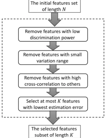
The proposed approach contains four stages each of which tries to purify/reduce the original features set of length 𝑁. The goal is to select at most 1 ≤ 𝐾 ≤ 𝑁 features. Figure 1 displays the flowchart of the proposed approach.
The four stages of the proposed approach are discussed in the following. Furthermore, a technique is employed to determine a reasonable minimum number of features. The method is discussed in section 2.5.
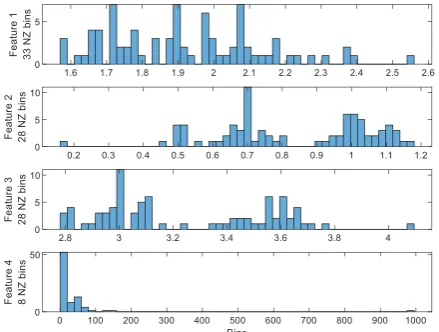
2. 1. Stage 1: Discrimination Ability The features with low discrimination ability are disregarded. By our definition, a feature with a lot of flat areas in its plot across different samples has low discrimination power. Figure 2 depicts a sample plot of four different features and output values over samples. It is evident that the output value is growing across samples. A discriminative feature should change across samples too.
In order to detect the flat areas in a feature plot, the histogram of the feature is calculated. A feature that has non-zero bins count smaller than a threshold 𝛽, is marked as a non-discriminative feature and will be removed. 𝛽 = 𝑓𝑙𝑜𝑜𝑟(2
5 𝑏𝑖𝑛𝑠 𝑐𝑜𝑢𝑛𝑡) is an appropriate empirical threshold for the minimum number of non-zero bins. Feature 4 in Figure 2 is an example of a non-discriminative feature that has many flat areas that are detectable in the histogram represented in Figure 3.
Figure 1. Flowchart of the proposed approach
The initial features set of length 𝑁
The selected features subset of length 𝐾 Remove features with low
discrimination power
Remove features with small variation range
Remove features with high cross-correlation to others
Figure 2. A sample plot of features and the output value across all samples
Figure 3. The histogram of features provided in Figure 2. For a better representation, 50 bins are considered for all features. 𝑁𝑍 means Non-Zero
2. 2. Stage 2: Variation Range To compute features with a small variation range, the first step is to normalize the features set. Min-Max normalization is used, as stated in Equation (1).
𝑧𝑖=
𝑥𝑖−min (𝑥)
max(𝑥)−min (𝑥) , (1)
where 𝑥𝑖= (𝑥1, 𝑥2, … , 𝑥𝑀) is the ith feature, 𝑀 is the number of samples, and 𝑧𝑖 is the ith normalized feature.
In the second step, the features with a standard deviation smaller than a threshold 𝛿 will be omitted. We utilized 𝛿 = 0.15 as a good empirical threshold.
2. 3. Stage 3: Cross-correlation The relevancy of a feature is measured based on the characteristics of the data, not by its value. There are some statistical measures to show the relations between the features [1, 27]. Usually, there are some features that have a high correlation with each other. There are different types of
correlation, but the one we were interested in was a linear correlation. If there would be some highly correlated features, there is no need to include them all in the final features subset. So we can select one of them and eliminate the others. In order to filter out this kind of features, the cross-correlation between feature 𝑥𝑖, 𝑖 ∈ {1, … , 𝑁} and other features 𝑥𝑗, 𝑗 ∈ {1, … , 𝑁} − {𝑖} is measured, and if the result was greater than a threshold 𝜏, the feature 𝑥𝑖 or 𝑥𝑗 will be eliminated. 𝑁 represents the number of features. The employed experimental threshold value was 𝜏 = 0.99. Between 𝑥𝑖 and 𝑥𝑗, the one with higher cross-correlation to the output, will be kept. Algorithm 1 demonstrates the pseudo-code for the proposed method. xcorr(𝑥𝑖,𝑥𝑗) calculates the cross-correlation between vector 𝑥𝑖 and 𝑥𝑗.
Algorithm 1. The proposed algorithm to remove features with high cross-correlation
𝑋 = feature set for all samples 𝑂 = the output vector
for 𝑥𝑖 in 𝑋
for 𝑥𝑗 in 𝑋 − {𝑥𝑖} if xcorr(𝑥𝑖,𝑥𝑗) > 𝜏
if xcorr(𝑥𝑖,𝑂) > xcorr(𝑥𝑗,𝑂) 𝑋 = 𝑋 − [𝑥𝑗]
else
𝑋 = 𝑋 − [𝑥𝑖] end if
end if end for end for
2. 4. Stage 4: The Best 𝑲 Features In the previous stages, a number of features were eliminated. From the remaining ones, 𝐾 features will be selected. To pick the approximately best features, a customized GA is proposed. The implemented binary generic algorithm tries to pick at most 𝐾 features which minimize the proposed cost function 𝑐(𝑣) as presented in Equation (2).
𝑐(𝑣) = {1 + 𝑥𝑐𝑜𝑟𝑟′(𝑣) + 𝑁𝑅𝑀𝑆𝐸 𝑖𝑓 𝑅
2= 0
(1 − 𝑅2) + 𝑥𝑐𝑜𝑟𝑟′(𝑣) 𝑖𝑓 𝑅2≠ 0 (2)
where 𝑅2 is the coefficient of determination measured, as shown in Equation 3. 𝑅2 is employed to compute the accuracy of the estimation by the selected features. 𝑦𝑖 and 𝑓𝑖 are the ith output value and estimated value respectively, and 𝑦̅ is the average of y. The xcorr' measures the average cross-correlation between the selected features (Equation 4). NRMSE is the normalized root mean square error calculated, as stated in Equation (5).
𝑅2= 1 −∑ (𝑦𝑖 𝑖−𝑓𝑖)2
∑ (𝑦𝑖 𝑖−𝑦̅)2 (3)
𝑥𝑐𝑜𝑟𝑟′(𝑣) = |𝑥𝑐𝑜𝑟𝑟(𝑣𝑖,𝑣𝑗)
𝑁𝑅𝑀𝑆𝐸 =√ 1 𝑛∑ (𝑦𝑖 𝑖−𝑓𝑖)2
𝑦̅
(5)
The 𝑅2 output is in the range of [0-1]. 𝑅2= 0 means a completely wrong estimation, and 𝑅2= 1 indicates an exact estimation. xcorr' is in range of [0,1]. xcorr'=0 shows no cross-correlation. In order to estimate how bad a feature set is, NRMSE term will be added to Equation 2 just when 𝑅2= 0. In other circumstances, 𝑅2 will be sufficient, because it contains an approximation of NRMSE.
In the proposed GA, a chromosome includes an N-dimensional vector of boolean values which determines whether a feature is selected or not. The goal of the GA is to pick at most 𝐾 features, so a chromosome cannot have more than 𝐾 ones. If a newly generated chromosome has more than 𝐾 ones (𝐿), 𝐿 − 𝐾 values are randomly chosen and set to zero. The flowchart of the proposed GA is provided in Figure 4.
K-fold cross-validation is employed for the cost function calculation in the proposed GA as the following: I) The sample set is divided into K folds, II) The cost function is evaluated K times each of which utilizes K-1 folds for training and 1 fold for testing, and III) The results are averaged over K as the final cost function value. The parameters configuration employed in the proposed GA is demonstrated in Table 1.
2. 5. Optimal Minimum Number of Features A technique is recommended to select a reasonable minimum number of features [28]. This technique
Figure 4. The flowchart of the proposed genetic algorithm. The flow order of the algorithm is presented with numbers from 1 to 5
TABLE 1. The proposed GA parameters configuration
Parameter Value
Population size 10000
Termination criterion 1000 epochs
Crossover probability 0.7
Mutation probability 0.2
Tournament size 3
divides the sample set into two training, and test sets; and then defines three criteria: training estimation accuracy (𝑇𝐸𝐴), testing estimation accuracy (𝑇𝐴𝑅), and training error (TE). Practically, this technique wraps around the proposed GA which, is called for different values of K starting from 1 to 𝑁 (the number of features). In each iteration, the three criteria are evaluated and plotted, until these three lines remain almost parallel to the X-axis. TEA and TAR are calculated using 𝑅2 measure on the training and test set, respectively. TE is computed by NRMSE measure on the training set.
Figure 5 displays an example with values of 𝐾 = {1,2, … ,7}. For each value of K, the GA is called, and the criteria are measured and plotted. After 𝐾 = 4 point, all the lines are approximately parallel to the X-axis. So 𝐾 = 4 is picked as the optimal minimum number of features.
3. THE EXPERIMENTAL RESULTS
We have been provided two chemical datasets by Nekoei et al. [28] that were suited to be analyzed by the proposed approach. Both of these datasets have a low sample size with high-dimensional data. In the following, the two case studies based on these datasets are discussed in detail. Table 2 presents the proposed algorithm configuration used for both case studies.
Figure 5. An example demonstrating the three proposed criteria for finding the optimal minimum number of features [28]
Generation of new population
Mutation Crossover
Tournament Selection Generation of offspring
Computation of the regression coefficients for a linear model with the selected features and k’-1 folds (training set)
Calculation of the cost function fold (test set)
th
using the k
R
ep
ea
t
un
ti
l all
f
ol
ds
ar
e
us
ed
as
the
tes
t
set
Evaluation of population
Average cost function
R
ep
ea
t
for numb
er
of
ep
oc
hs
1
2
3
4
The selected feature
5
TE TEA TAR
Number of features
Functi
on
value [
0
-1
TABLE 2. The proposed algorithm parameters configuration
Parameter Value
𝛽 20 from 50 bins
𝛿 0.15
𝜏 0.99
3. 1. Chemical Molecules Case Study The first case study is focused on a chemical molecules dataset, which contains 81 molecules with 1056 physicochemical properties or theoretical molecular descriptors (Figure 6). Every molecule has a response value measured based on the descriptors. The goal is to find a linear QSAR-based model to predict the response variable with a subset of features. The descriptors and response values are all numerical and their numerical values may not be in the same range.
Figure 7 shows the minimum number of descriptors suggested by the proposed technique. The average values of 𝑅2 measure over training and test sets for different numbers of selected features and the selected features itself are summarized in Table 3.
Figure 6. The chemical molecules dataset with 81 samples (m), 1056 features (a), and a response value (f)
Figure 7. The optimal number of descriptors in chemical molecules dataset
TABLE 3. The average values of 𝑅2 measure, and the selected
descriptors indices for different numbers of descriptors of chemical molecules dataset. The features name are displayed for the selected descriptors (fourth row)
Num of
features Selected feature indices Average 𝑹
𝟐
1 [188] 0.880
2 [75,188] 0.919
3 [188,413,682] 0.928
4 [188,281,413,936]
[𝑉𝐸𝐴1, BELv1, GATS2e, H5p] 0.942
5 [188,413,684,778,990] 0.945
6 [188,384,412,650,684,741] 0.946
It is evident from Table 3 that by selecting more than four features, there will be slight variations in 𝑅2 response values. Therefore, the suggested optimal minimum number of features is four. It is worth noting that the feature number 188 must have a significant contribution to the linear model, as it is selected in all six suggested features set.
The linear model found by the proposed GA for 𝐾 = 4 using multiple linear regression (MLR) is given by Equation (6). The model was used to predict the response variable, and the average result measured by K-fold cross-validation is compared with a feed-forward neural network (NN) once trained with the initial features set, and once trained with the reduced features set. The comparison results are presented in Table 4. Additionally, the regression plot is demonstrated in Figure 8.
𝑓 = −0.403 (𝑽𝑬𝑨𝟏) − 0.454 (𝐁𝐄𝐋𝐯) +
0.022 (𝐆𝐀𝐓𝐒𝟐𝐞) + 0.880 (𝐇𝟓𝐩) + 1 (6)
3. 2. Chemical Drugs Case Study This case study includes a chemical drugs dataset with 103 samples of 1482 dimensional data. Like the previous dataset, each sample has a response value. The goal is to build a linear model to predict the response variable employing just a subset of descriptors.
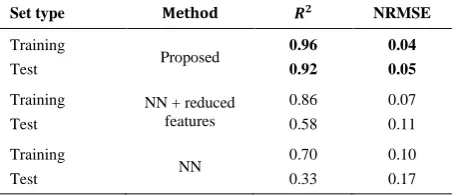
TABLE 4. The average 𝑅2 and NRMSE measures of the built
model of the chemical molecules case study using K-fold cross-validation, compared against NN
Set type Method 𝑹𝟐 NRMSE
Training
Test Proposed
0.96 0.92
0.04 0.05
Training
Test
NN + reduced features
0.86
0.58
0.07
0.11
Training
Test NN
0.70
0.33
0.10
(a) Training data
(b) Test data
Figure 8. The regression plot of the built model of chemical molecules case study on (a) training and (b) test sets
The optimal minimum number of features suggested for this dataset, as depicted in Figure 9 is six. Moreover, the average values of 𝑅2 term over training and test sets for 1 to 6 selected features are presented in Table 5.
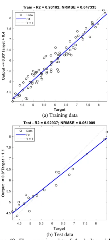
The linear model suggested by the proposed GA for 𝐾 = 6 using the MLR is given by Equation (7). Similar to the previous section, the average prediction accuracy and error of the model is compared with NN, and the results are provided in Table 6. Also, the regression plot is shown in Figure 10.
𝑓 = 5.333 (𝑇(𝑂. . 𝐹)) + 0.021(GGI7) + 0.700 (JGT) − 12.126 (MATS7v) −
37.334 (PCWTe) − 0.234 (RDF065m)
(7)
Figure 9. The optimal number of descriptors in chemical drugs dataset
TABLE 5. The average values of 𝑅2 measure, and the selected
descriptors indices for different numbers of descriptors of chemical drugs dataset. The features' names are displayed for the selected descriptors (sixth row).
Num of
features Selected feature indices
Average
𝑹𝟐
1 [103] 0.633
2 [61,550] 0.825
3 [136,569,892] 0.849
4 [415,524,788,1220] 0.877
5 [415,524,788,901,1355] 0.898
6
[285,401,415,462,524,670] [T(O..F), GGI7, JGT,
MATS7v, MATS7v, PCWTe, RDF065m]
0.930
TABLE 6. The average 𝑅2 and NRMSE measures of the built
model of the chemical drug case study using K-fold cross-validation, compared against NN
Set type Method 𝑹𝟐 NRMSE
Training
Test Proposed
0.93 0.93
0.05 0.06
Training Test
NN + reduced features
0.87 0.65
0.07 0.10
Training
Test NN
0.73 0.40
0.1 0.16
(a) Training data
(b) Test data
Figure 10. The regression plot of the built model of chemical drugs case study on (a) training and (b) test sets
of around 70% on training data (Tables 4 and 6). Although, due to the small number of samples, NN overfits and thereupon, shows a sudden accuracy decrease over the test data. By reducing the number of input features drastically, the performance of NN grows significantly on both datasets. Still, the best result is earned by the proposed approach, which utilizes multiple linear regression internally. As can be seen in Tables 4 and 6, the accuracy of the proposed method on the training and test sets are very close together. It indicates that overfitting has not happened when training the model, and the built model is robust and accurate
4. CONCLUSION
In this work, a heuristic hybrid approach for feature selection is proposed. The approach reduces the number
of features significantly in four consecutive stages. In the early stages, some of the irrelevant and less discriminative features are omitted. In the final stages, the approximately best feature subset of length 𝐾 is chosen by a GA which uses a customized cost function. The proposed cost function maximizes the prediction accuracy and minimizes the prediction error, and the cross-correlation between the selected features subset simultaneously.
Two case studies with high-dimensional data were analyzed to indicate the performance of the proposed approach. Firstly, the proposed method was applied to a chemical molecules dataset and reduced the number of features from 1056 to 4 with a prediction accuracy of 𝑅2= 0.92. Secondly, a similar configuration is used for the next dataset that led to the reduction of 99.6 percent of the features with a prediction accuracy of 𝑅2= 0.93. The experimental results indicate that the proposed method is better suited to be used for small sample sets with high dimensional data than neural networks. Additionally, our approach can be employed as a pre-processing step in other methods. As we demonstrated the performance boost of NN when injected with our reduced features set.
5. REFERENCES
1. Venkatesh, B., Anuradha, J., ‘A Review of Feature Selection and Its Methods’, Cybernetics and Information Technologies, Vol. 19, No. 1, (2019), 3–26.
2. Li, J., Cheng, K., Wang, S., et al., ‘Feature Selection: A Data Perspective’, ACM Computing Surveys, Vol. 50, No. 6, (2018), 94.
3. Cai, J., Luo, J., Wang, S., Yang, S., ‘Feature selection in machine learning : A new perspective’, Neurocomputing, Vol. 0, (2018), 1–10.
4. Li, J., Liu, H., Science, C., ‘Challenges of Feature Selection for Big Data’, IEEE Intelligent Systems, Vol. 32, No. 2, (2017), 9– 15.
5. Jovi, A., Brki, K., Bogunovi, N., ‘A review of feature selection methods with applications’, , in ‘38th International Convention on Information and Communication Technology, Electronics and Microelectronics’ (2015), 1200–1205
6. Asir, D., Appavu, S., Jebamalar, E., ‘Literature Review on Feature Selection Methods for High-Dimensional Data’,
International Journal of Computer Applications, Vol. 136, No.
1, (2016), 9–17.
7. Mazimpaka, J.D., Timpf, S., ‘Trajectory data mining : A review of methods and applications’, Journal of Spatial Information
Science, Vol. 13, (2016), 61–99.
8. Hamidi, H., Daraei, A., ‘Analysis of Pre-processing and Post-processing Methods and Using Data Mining to Diagnose Heart Diseases’, International Journal of Engineering-Transactions
A: Basics, Vol. 29, No. 7, (2016), 921–930.
9. Kumar, S., Sahoo, G., ‘A Random Forest Classifier based on Genetic Algorithm for Cardiovascular Diseases Diagnosis’,
International Journal of Engineering-Transactions B:
Applications, Vol. 30, No. 11, (2017), 1723–1729.
Selection’, (CRC Press, 2007)
11. Liu, H., Setiono, R., ‘A Probabilistic Approach to Feature Selection - A Filter Solution’, , in ‘Proceedings of 13th International Conference on Machine Learning’ (1996), 319–327 12. Fayyad, U.M., Irani, K.B., ‘The attribute selection problem in
decision tree generation’, , in ‘AAAI’ (1992), 104–110 13. Kalpana, P., Mani, K., ‘A New Hybrid Framework for Filter
based Feature Selection using Information Gain and Symmetric Uncertainty’, International Journal of
Engineering-Transactions B: Applications, Vol. 30, No. 5, (2017), 659–667.
14. Ch, V., Asvestas, P.A., Delibasis, K.K., Matsopoulos, G.K., ‘A classification system based on a new wrapper feature selection algorithm for the diagnosis of primary and secondary polycythemia’, Computers in Biology and Medicine, Vol. 43, (2013), 2118–2126.
15. Kohavi, R., John, H., ‘Wrappers for feature subset selection’,
Artificial Intelligence, Vol. 97, (1997), 273–324.
16. Dy, J.G., Brodley, C.E., ‘Feature Subset Selection and Order Identification for Unsupervised Learning’, , in ‘Proceedings of 17th International Conference of Machine Learning’ (2000), 247– 254
17. Yang, Y., Pedersen, J.O., ‘A Comparative Study on Feature Selection in Text Categorization’, , in ‘Proceedings of 14th International Conference on Machine Learning’ (1997), 412–420 18. Mohsenzadeh, Y., Sheikhzadeh, H., Member, S., Reza, A.M., Member, S., Kalayeh, M.M., ‘The Relevance Sample-Feature Machine : A Sparse Bayesian Learning Approach to Joint Feature-Sample Selection’, IEEE Transactions on Cybernetics, Vol. 43, No. 6, (2013), 2241–2254.
19. Yan, K., Zhang, D., ‘Feature Selection and Analysis on Correlated Gas Sensor Data with Recursive Feature Elimination’,
Sensors & Actuators: B. Chemical, Vol. 212, (2015), 353–363.
20. Jain, A., Zongker, D., ‘Feature Selection Evaluation, Application, and Small Sample Performance.pdf’, IEEE Transactions on
Pattern Analysis and Machine Intelligence, Vol. 19, No. 2,
(1997), 153–158.
21. Talavera, L., ‘Feature Selection as a Preprocessing Step for Hierarchical Clustering’, , in ‘Proceedings of 25th International Conference of Machine Learning’ (1999), 389–397
22. Das, S., ‘Filters , Wrappers and a Boosting-Based Hybrid for Feature Selection’, , in ‘Engineering’ (2001), 74–81
23. Biesiada, J., Duch, W., ‘Feature Selection for High-Dimensional Data – A Pearson Redundancy Based Filter’, , in ‘Advances in Soft Computing’ (2007), 242–249
24. Estévez, P.A., Member, S., Tesmer, M., Perez, C.A., Member, S., Zurada, J.M., ‘Normalized Mutual Information Feature Selection’, IEEE Transactions on Neural Networks, Vol. 20, No. 2, (2009), 189–201.
25. Vinh, L.T., Thang, N.D., Lee, Y., ‘An Improved Maximum Relevance and Minimum Redundancy Feature Selection Algorithm Based on Normalized Mutual Information’, , in ‘Proceedings of 10th IEEE/IPSJ International Symposium on Applications and the Internet’ (2010), 395–398
26. Quinlan, J.R., ‘Bagging, Boosting, and C4.5’, AAAI/IAAI, Vol. 1, (2006), 725–730.
27. Gheyas, I.A., Smith, L.S., ‘Feature Subset Selection in Large Dimensionality Domains’, Pattern Recognition, Vol. 43, No. 1, (2010), 5–13.
28. Nekoei, M., Mohammadhosseini, M., Pourbasheer, E., ‘QSAR study of VEGFR-2 inhibitors by using genetic algorithm-multiple linear regressions (GA-MLR) and genetic algorithm-support vector machine (GA-SVM): A comparative approach’, Medicinal
Chemistry Research, Vol. 24, No. 7, (2015), 3037–3046.
Feature Selection for Small Sample Sets with High Dimensional Data Using Heuristic
Hybrid Approach
M. Biglari, F. Mirzaei, H. Hassanpour
Computer Engineering and IT Department, Shahrood University of Technology, Shahrood, Iran
P A P E R I N F O
Paper history: Received 28 August 2019
Received in revised form 16 January 2020 Accepted 16 January 2020
Keywords: Feature Selection Data Mining Regression
High Dimensional Data Evolutionary Methods
هدیکچ
هداد اب ههجاوم رد هنومن دادعت رگا هژیو هب ،لااب داعبا اب یاه
ییلااب تیمها زا یگژیو باختنا ،دشاب مک اه .تسا رادروخرب
شور جارختسا یاه
.تشاد دنهاوخن یلوبق لباق درکلمع ،یطیارش نینچ رد یگژیو هنومن دادعت دوجو اب
یگژیو دادعت و مک یاه یوجتسج یاضف شواک ،دایز یاه
یریگدای و هدش راوشد گرزب اب
هنومن دادعت ماجنا یگداس هب ،مک اه .تسین ریذپ
هکبش ،ور نیا زا شور و یبصع یاه
هتسد یاه یور رب یدنب
هداد عون نیا .دنراد یفیعض درکلمع اه یگژیو دادعت دیدش شهاک یارب دیدج یبیکرت یگژیو باختنا شور کی ،هلاقم نیا رد
هدش هئارا اه
شیپ تقد یئزج شهاک هب رجنم اهنت هک .دش دهاوخ راظتنا دروم یجورخ ینیب
یم لمع هلحرم دنچ رد یداهنشیپ شور ادتبا رد .دنک
یگژیو یگژیو سپس و هدش فذح مک زیامت تردق اب طبترمان یاه یم طخ ،دنتسه دودحم تارییغت هزاب یاراد هک ییاه
هلحرم رد .دنروخ
یگژیو هعومجم ره نیب زا ،دعب یم هتشاد هگن ،تسا یجورخ رادقم اب یگتسبمه نیرتشیب یراد هک یگژیو کی اهنت ،لااب یگتسبمه اب اه
.دوش
،ییاهن ماگ رد یگژیو هب یشرافس هنیزه عبات اب کیتنژ متیروگلا کی
یگژیو هعومجم نیرتکچوک ات هدش لامعا هدنامیقاب یاه ار اراک یاه
.دنیزگرب توافتم هلئسم ود ،یداهنشیپ شور ییاراک شیامن یارب
ابیرقت دادعت اب 100
یگژیو دادعت و هنومن زا رتشیب یاه
1000 ، هعلاطم دروم
هتفرگ رارق اتن .دنا زا شیب شهاک ،هدش ماجنا تاشیامزآ جی 99
یگژیو دادعت یدصرد یم ناشن ار اه
شیپ تقد هک یلاح رد ،دهد یجورخ ینیب
![Figure 5. An example demonstrating the three proposed criteria for finding the optimal minimum number of features [28]](https://thumb-us.123doks.com/thumbv2/123dok_us/13352.2001247/4.595.64.280.474.716/figure-example-demonstrating-proposed-criteria-finding-optimal-features.webp)