An Algorithm based on Predicting the Interface in Phase Change Materials

Please cite this article as: A. M. Jadidi, M. Jadidi, An Algorithm based on Predicting the Interface in Phase Change Materials, International Journal of Engineering (IJE), IJE TRANSACTIONS B: Applications Vol. 31, No. 5, (May 2018) 799-804

International Journal of Engineering

J o u r n a l H o m e p a g e : w w w . i j e . i r

An Algorithm based on Predicting the Interface in Phase Change Materials

A. M. Jadidi*a_{, M. Jadidi}b

a _{Department of Mechanical Engineering, Semnan University, Semnan, Iran} b _{Department of Mechanical Engineering, Griffith University, Australia}

P A P E R I N F O

Paper history:

Received 29 May 2017

Received in revised form 13 February 2018 Accepted 08 March 2018

Keywords: Phase Change Material Numerical Simulation Finite Difference Stephan Problem

A B S T R A C T

Phase change materials are substances that absorb and release thermal energy during the process of melting and freezing. This characteristic makes phase change material (PCM) a favourite choice to integrate it in buildings. Stephan problem including melting and solidification in PMC materials is an practical problem in many engineering processes. The position of the moving boundary, its velocity and the temperature distribution within the domain are important for these applications. Well known numerical techniques have difficulties with time-dependent boundary conditions. Therefore, fine mesh and small time steps are needed to obtain accurate solutions. There are two main approaches to solve the Stefan problem: front-tacking and variable grid method. The most existing methods are not applicable to all situations and they cannot be easily implemeted in two-dimensional or three-dimensional geometries and all boundary conditions. In this paper, we proposed an algorithm to solve one-dimensional Stefan problem in all kind of boundary condition; also it can be easily extended for 2D and 3D Stephan problems using finite difference method. For validation, the results are compared with exact solution of constant boundary condition. Afterward, periodic boundary condition is considered. The results showed significant relationship between numerical and exact solution, and the maximum error was approximately 0.4%.

doi: 10.5829/ije.2018.31.05b.15

NOMENCLATURE

T Temperature _k Time index

0

T Temperature at x=0 n Position index

m

T PCM melting temperature * Predicted value

b

T Boundary temperature N Number of time steps

t

 Time step t Time

x

 Space step x Position

x* Position predicted value A, D matrices

s

Interface location between solid and liquid phases Greek Symbols

k Conductivity (Wm/K)  Density (kg/m3)

r Latent heat (kj/kg)



Convergence criteria

a Thermal diffusivity  ,  Coefficient

1. INTRODUCTION1

Increasing demand for thermal comfort can result in rising energy consumption in buildings and many other applications. PCM are substances that absorb and

*Corresponding Author Email: [email protected](A. M. Jadidi)

release thermal energy during the process of melting and freezing. This characteristic makes PCM a suitable choice to integrate it in building walls. The use of PCM integrated into walls is a way to enhance the thermal storage capacity of buildings.

This problem is generally referred as phase-change or moving-boundary problem. The position of the moving boundary, its velocity and the temperature distribution within the domain are important for these applications.

Since the solid-liquid interface is time-dependent and must be determined as a part of the solution, the problems are highly nonlinear and become complicated except for a limited number of special cases. Therefore, these problems in the most cases are required to be solved numerically.

Due to difficulties in obtaining an analytical solution, various numerical techniques have been developed over last decades (including finite element, finite difference and integral methods) to solve moving boundary problem. Generally, in terms of accuracy and efficiency, the choice between various finite element, finite difference and integral methods for the solution of a particular Stefan problem is not always clear, due to their specific advantages and limitations.

A two-dimensional transient axi-symmetric model has been developed to study the effect of thermal and geometric parameters on cyclic heating and cooling modes of a phase-change thermal energy storage system by Adami [4]. The Gauss-Seidel iterative method with over-relaxation is used to solve the non-linear simultaneous difference equations [4].

A numerical simulation of refrigeration cycle with PCM heat exchanger carried out by Bakhshipour et al. [5] in cylindrical coordinate using finite volume approach. They investigated the effects of type of refrigerant, PCM heat exchanger length, PCM heat exchanger tube diameter, PCM thickness and mass flow rate of refrigerant. Costa et al. [6] have used the enthalpy formulation with a fully implicit finite difference method to analyse numerically the thermal performance of latent heat storage. The method takes into account both conduction and convection heat transfer in a one-dimensional model. The method used was validated by comparing the results with other analytical and numerical results found from the literature. The conclusion is that the method is useful for designing a thermal energy storage [6]. To obtain physical validation in PCM material, the numerical simulation has been carried out using enthalpy method and effective heat capacity method [7]. The numerical results compared with the experiment results achieved by thermocouples mounted inside the PCM.

Optimal homotopy asymptotic method (OHAM) has been used to solve one dimensional stefan problem by Rajeev et al. [8]. An approximate solution is obtained using the OHAM to find the solutions of temperature distribution in the domain 0 ≤x≤s(t) and interface’s tracking or location with the help of Taylor series.

Numerical techniques are specially known to have difficulties with time-dependent boundary conditions. Therefore, fine mesh and small time steps are needed to

obtain accurate solutions. Unfortunately, there is not enough research about the Stefan problem with time- dependent boundary conditions [9].

There are two main approaches to the solution of the Stefan problem [9]. One is the front-tracking method in which the position of the phase boundary will be tracked continuously. Alternatively, variable grid methods provide the way to track the phase front explicitly [10]. In variable grid methods, time step and space grid are variable.

For moving boundary problems, numerical methods have been compared in various studies [11].

In one algorithm proposed in literature [12], instead of front tracking, moving interface locations is preset and use these location coordinates as the grid points to find out the arrival time of moving interface. Applying this approach can help to avoid the difficulty in mesh generation. This algorithm encounters serious challenges in time-dependent boundry conditions because of presetting interface location and finding arrival interface time.

A mathematical model is proposed to simulate the coupled heat transfer equation and Stefan condition occurring in moving boundary problems like the solidification process in the continuous casting machines [13].

In this study, the finite difference approach and the boundary immobilization method has been selected to find the position of moving interface and the temperature distribution. Most of the proposed methods cannot be easily implemeted in two / three-dimensional geometries and all boundary conditions. In this paper, we proposed an algorithm to solve one-dimensional Stefan problem in all kind of boundary conditions. This method can be easily extended for 2D and 3D Stephan problems. For this reason, this method presets arbitrary time steps and then it finds interface location.

To evaluate this new algorithm, both constant and time-dependent periodic boundary conditions have been considered, and the finite difference approach has been used in order to determine the temperature distribution and phase boundary during the process. Under constant boundary conditions, there is a significant relationship between the present numerical solution results and the exact solution one. To achieve qualitative results, grid independency is checked to find a suitable grid number with minimum error. The algorithm is also very straightforward and efficient for its finite difference formulation.

2. NUMERICAL ALGORITHM

this algorithm is predicting the boundary between the solid and liquid phase in each non-uniform time step. Also, at the same time steps can be selected. The discretization is based on finite difference schemes. The governing equation for one-dimensional heat transfer through a PCM is:

2

2

1 0

1

1

1

( , ) at x = 0 and t > 0

. . ( , ) at x = s(t) and t > 0

at x = s(t) and t > 0 m

T T

x a t

T x t T

B C T x t T

T s

k r

x  t

 _ 

 



   



  



 _{ }

   

 



(1)

where, T is temperature, t is time, T0 is the temperature at x=0, Tm is the PCM melting temperature,  is the PCM density, k is thermal conductivity, a is thermal diffusivity, r is latent heat of PCM and s is the interface location between solid and liquid phases. The first boundary condition is constant temperature and third boundary condition is a nonlinear boundary condition coupled with governing equation. One of the main advantages of this algorithm is its ability to execute in every boundary condition like periodic and other types of boundary conditions. It is assumed that time steps are given as follows:

1

1 1 0

2

2 2 1

1

...

k

k k k

t t t t

t t t t

t t t  t

       

   

(2)

Also, the interface in each time step defines as

s

_nk that

k is time index and n is the position index. If the PCM warms up at x=0 by T0 temperature, and heat will be diffused through PCM and melting process will start. This process is illustrated in Figure 1.

Central scheme and Euler's first order scheme are used for discrete diffusion terms , and time derivative terms respectively. In the first time step, the length of melted zone can obtain discretizing the third boundary condition as Equation (3):

1 1 1 0

1 0 1 1

1 1

1 1 1 1 1

1 0 1 1 1 0

-k r

T =T , T =T and x =s then m o s ( m)

T T s s

T s

k r

x t x t

k

t T T

r

 



 

 

    

  

    

(3)

The interface between liquid and solid phases at first time step will be easily predicted using only Stephen's boundary condition. But, in the next time steps to achieve this purpose, one dimensional heat transfer equation must be discretized based on Equation (4). As seen, a non uniform grid is used because of the non linear nature of Stephen's problem.

1 1

1 1 1

2 _{1 1}

2 2

2

1 2

1

1 1

1 1 1 2 2

2 1 1

2 2 1 1

2

1 2 1 2 2 1

1

2 1 2

1 1 1

2 2

and

( )

2

2

2 m o

m

T T

T T T

x x

x x x x

T T

T T

T T

T

x x x x x x x x

T T T T

T

t t t

 

 



 _   _{ } _{ }

  _{  }

    

  



   _{ }

 

 _    _{   }

 

        _   _

 

 

 

 

 _{ }

  

(4)

Simplifying Equation (4), a relation like T12 will

be obtained that α and β are as Equation (5).

*

2

2 1

1 1

* *

2 1 2 2 1

1 1 1

2 m o

a t

x x

T

T T

a t x x x x





 

  



 

 

  _  _

    _  _

(5)

The * index indicates predicted values. With a similar procedure as mentioned in the first time step, the Δx2 can be found as Equation (6).

2

2 2 ( 1 m)

k

x t T T

r



    (6)

At the second time step, to start solution procedure, first a guess for *

2 x

 is necessary. After predicting * 2 x

 , α and β will be calculated explicitly using Equation (5).

Afterward 2

1

T will be obtained from T12.

Substituting 2 1

T in Equation (6) results in a new value for x₂. The error criteria now can be found

subtracting * 2 x

 fromx₂.

*

2 2

Error   x x epsilon (7)

If error value was smaller than epsilon, convergence criteria are met and this step will be finished, otherwise,

* 2 2

x x

   _{and this procedure repeats until the}

convergence criteria are met.

In the next steps, as the temperature of nodes couples together, the previous methods do not work correctly. Discretization of 1D heat equation results in Equation (8). Spatial derivative of Equation (1) is replaced with central difference approximation at n-1'th grid position. The n varies from 2 to k and k is current time step.

2 1

1 1

1 1 1

1

1 1

2

( )

2 2 1

( ) ( )

2

( )

1

k k k

n n n

n n n

k

n n n n n n

n n n

k n k

aT bT cT d

a

x x x

b

x x x x x x at

c

x x x

d T

at

 

 

  

  

  

 

   

  

       

 

   



(8)

In the other hand, the above equations can be summarised as a system of the linear equation like AT = D. A and D are matrices which elements can be found in Equation (8) and T is the nodes temperature matrix. The convergence criteria at current time step can be found from third boundary condition at the interface of two phases, as expressed in Equation (9):

1

( )

new k k k

k k k

k

x t T T

r



 

   (9)

The algorithm of solving such a system can be listed as:

 A guess for x_kand solving AT = D according to Thomas algorithm based on Equation (8).

 Finding new

k

x

 based on Equation (9).

 Checking convergence criteria x_knew  xold_k .

 If convergency happened, this algorithm finishes,

else new

k k

x x

   and this algorithm repeats from the first line.

The advantages of this algorithm are: 1. Grid generation has removed completely.

2. Compatible with different kinds of boundary

conditions like time dependent and etc.

3. The algorithm can be easily extended to solve Stephan problem in 2D and 3D.

4. This algorithm is flexible and easy to use.

3. RESULT

In this section, our algorithm results have been presented. Initially, to validate and verify the proposed algorithm, the analytical results of melting an aluminum wall under constant temperature are compared with numerical results. Then, two different boundary conditions (periodic boundary condition and constant boundary condition) are numerically investigated during a day. The PCM wall type is CaCl2.6H2O.

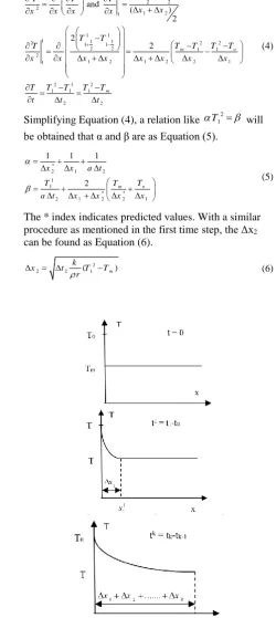
In Figure 2, the length of melted zone is shown at different times and the analytic solution is presented to validate the numerical model. Melting process of aluminum is considered. The melting temperature of aluminum is Tm=931 K and boundary temperature is Tb=1073 K. The other physical properties of aluminum are given as follow: r = 396 kJ/kg, ρ = 2380 kg/m3 _{, k =} 215 Wm/K , c = 1130.44 J kg/K. The convergence criteria are ε = 1e-5. As shown in Figure 2, numerical results are in good agreement with an exact solution that confirms the high accuracy of the numerical method. The maximum error happened in the first time and maximum error is approximately 0.4%.

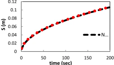
In Figures 3 and 4 grid independency for two different boundary conditions (Figure 3 shows grid independency in Tb=cte and Figure 4 presents it when periodic B.C. applied) are shown.

For this reason, a PCM wall with CaCl2.6H2o is selected. It is completely clear that in both states grid independency happens when the number of grid is N = 96. The temperature periodic function is as equation (10). Where Tb is boundary temperature, Tm presents melting temperature, N is the number of time steps and n = 1, 2, …, N. It should be mentioned that all next results obtained with N = 96 when grid independency happens.

Figure 2. The comparison of numerical results with exact solution in melting process of aluminum under constant boundary condition

0 0.02 0.04 0.06 0.08 0.1 0.12

0 50 100 150 200

S (

m)

time (sec)

Figure 3. grid independency for constant boundary condition

Figure 4. grid independency for periodic boundary condition

0sin(2 )

b m

T T T  n N (10)

In Figure 5, temperature profile versus PCM melting zone length is shown in all day long (tfinall = 24 h). The boundary temperature is Tb = 314 °C and PCM (CaCl2.6H2O) melting temperature is Tm =304°C. Other physical properties of CaCl2.6H2O are: k = 0.53 W/mK, r = 187 kJ/kg, ρ = 1530 kg/m3 _{and cp = 2200 kJ/kg.K.} As shown in Figure 5 melting zone will be expanded when time increases. The maximum length of the melting zone is 5.51 cm and maximum rate of melting is in the first 6 hours where 2.64 cm of PCM melted. It can be easily understood that because of the nonlinear character of Stephen problem, PCM rate of melting is not the same in the same time steps. Therefore, using an algorithm based on non-uniform grid can result in more accurate results as this algorithm captures accurate melting zone length in PCM.

In Figure 6, temperature profile versus interface of the liquid and the solid region is shown. In this stage, periodic boundary condition is applied. As described in Equation (10) Tm is 304°C and T0 is 10 °C. Also, N is the number of time steps and n = 1, 2, …, N. Simulation is done in all day long. In first twelve hours, melting process (as Tb is greater than Tm) and in the second section of the day freezing process (because Tm is greater than Tb) are applied based on periodic boundary condition. As illustrated in a Figure 6, the rate of melting in first six hours is greater than second six hours and interface length (between solid and liquid region) is 3.17 cm.

Figure 5. Temperature profile in melting process of CaCl2.6H2O when boundary temperature is T0 = 314° C

Figure 6. Temperature profile in CaCl2.6H2O when boundary condition is periodic

In the other hand, optimum length for CaCl2.6H2O is 3.17 cm when periodic boundary condition is applied.

But in the second twelve hours, PCM will be frozen. It is obvious from Figures 4 and 6 that the interface length is the same in times having the same distance from t=12 hours. It can be found that in periodic boundary conditions, melting and freezing process in PCM happen at the same interface exactly. Also, temperature profiles are completely symmetry in freezing and melting process. This confirms that the results are obtained under periodic boundary condition. The inverse of melting process, the freezing rate in the second six hours is greater than first six hours.

4. CONCLUSION

A new algorithm was proposed in this paper to solve one-dimensional Stephan problem based on finite difference method. This algorithm main features capturing moving interface in arbitrary time steps without mesh generation and it was easy to apply in different boundary conditions.

To evaluate this algorithm, two different boundary conditions (BC) have been considered. First, constant temperature BC was applied that numerical results had well coincident with analytical solution in an aluminum 0

0.01 0.02 0.03 0.04 0.05 0.06

0 2 4 6 8 10 12 14 16 18 20 22 24

S (

m)

Time (hour)

N = 24 N = 48 N = 96

0 0.005 0.01 0.015 0.02 0.025 0.03 0.035

0 2 4 6 8 10 12 14 16 18 20 22 24

S (

m)

time (hour)

N=12 N=24 N=48 N=96

302 304 306 308 310 312 314 316

0 0.02 0.04 0.06

Temper

atu

re

s(m)

t=24 hour t=18 hour t=12 hour t=6 hour t=3 hour t=2 hour t=1 hour

294 298 302 306 310 314

0 0.01 0.02 0.03 0.04

Temper

atu

re

S (m)

wall. Then, time-dependent periodic BC was used in all day long and melting and solidification process in a PCM studied. The optimum PCM length captured approximately 3.17 cm for CaCl2.6H2O based on periodic boundary condition. Temperature profile versus interface location is linear in both boundary conditions. In melting and freezing process, the temperature profile was symmetry which confirms the validity of periodic boundary condition results. Also, Grid independency was checked to guaranty quality of numerical results.

The proposed algorithm can be easily developed for two-dimension and 3D applications. Algorithm accuracy was remarkable and maximum error was approximately 0.4% in the initial time step when constant temperature boundary condition was applied.

5. REFERENCES

1. Crank, J., "Free and moving boundary problems" (oxford science publications)", Clarendon Press, Oxford, UK, 1984, (1987).

2. Gupta, S., Laitinen, E. and Valtteri, T., "Moving grid scheme for multiple moving boundaries", Computer Methods in Applied Mechanics and Engineering, Vol. 167, No. 3-4, (1998), 345-353.

3. Mackenzie, J. and Robertson, M., "The numerical solution of one-dimensional phase change problems using an adaptive moving mesh method", Journal of Computational Physics, Vol. 161, No. 2, (2000), 537-557.

4. Adami, M., "Transient two-dimensional (RZ) cyclic charging analysis of space thermal energy storage systems (research

note)", International Journal of Engineering, 15 (2002), 205-210.

5. Bakhshipour, S., Valipour, M. and Pahamli, Y., "Parametric analysis of domestic refrigerators using pcm heat exchanger",

International Journal of Refrigeration, Vol. 83, (2017), 1-13. 6. Costa, M., Buddhi, D. and Oliva, A., "Numerical simulation of a

latent heat thermal energy storage system with enhanced heat conduction", Energy Conversion and Management, Vol. 39, No. 3-4, (1998), 319-330.

7. Lamberg, P., Lehtiniemi, R. and Henell, A.-M., "Numerical and experimental investigation of melting and freezing processes in phase change material storage", International Journal of Thermal Sciences, Vol. 43, No. 3, (2004), 277-287.

8. Kushwaha, M. and Singh, A.K., "A study of a stefan problem governed with space–time fractional derivatives", Journal of Heat and Mass Transfer Research (JHMTR), Vol. 3, No. 2, (2016), 145-151.

9. Savović, S. and Caldwell, J., "Finite difference solution of one-dimensional stefan problem with periodic boundary conditions",

International Journal of Heat and Mass Transfer, Vol. 46, No. 15, (2003), 2911-2916.

10. Marshall, G., "A front tracking method for one-dimensional moving boundary problems", SIAM journal on scientific and Statistical Computing, Vol. 7, No. 1, (1986), 252-263. 11. Furzeland, R., "A comparative study of numerical methods for

moving boundary problems", IMA Journal of Applied Mathematics, Vol. 26, No. 4, (1980), 411-429.

12. Wu, Z., Luo, J. and Feng, J., "A novel algorithm for solving the classical stefan problem", Thermal Science, Vol. 15, No. suppl. 1, (2011), 39-44.

13. Moghadam, A.J. and Hosseinzadeh, H., "Thermal simulation of solidification process in continuous casting", International Journal of Engineering-Transactions B: Applications, Vol. 28, No. 5, (2015), 812-821.

An Algorithm based on Predicting the Interface in Phase Change Materials

A. M. Jadidia_{, M. Jadidi}b

a _{Department of Mechanical Engineering, Semnan University, Semnan, Iran} b _{Department of Mechanical Engineering, Griffith University, Australia}

P A P E R I N F O

Paper history:

Received 29 May 2017

Received in revised form 13 February 2018 Accepted 08 March 2018

Keywords: Phase Change Material Numerical Simulation Finite Difference Stephan Problem

هديكچ

یم دازآ دامجنا و ندش بوذ یاه هسورپ یط رد ار ییامرگ یژرنا هک دنتسه یداوم هدنهد زاف رییغت داوم یا .دننک

صخشم ن داوم نیا ه هب ار

یم لیدبت ینامتخاس یاهدربراک رد بولطم باختنا کی رد دامجنا و بوذ دنیآرف لماش هک نافتسا هلاسم .دنک

داوم ت یم هدنهد زاف رییغ

-ماد رد امد عیزوت و نآ تعرس ،کرحتم زرم ناکم .تسا یسدنهم یاهدربراک زا یرایسب رد یدربراک هلاسم کی ،دشاب لح هن

د اهدربراک ر ی

اربانب .دنراد نامز هب هتسباو کرحتم زرم لیاسم رد یتلاکشم هدش هتخانش یددع یاهینکت .دراد تیمها داوم نیا ینچ نی

یاسم ن ب یل یار

ا دوجوم نافتسا هلاسم لح یارب هدمع شور ود .دنراد هاتوک ینامز یاهماگ و زیر هکبش هب زاین قیقد یلح نتشاد کی .تس

شور ،شور

یم ریغتم هکبش شور یرگید و هبل یبایدر یم راکب هزوح نیا رد هک ییاهشور رثکا .دشاب

هب و دنتسین عماج دنور یمن یناسآ

رد اهنآ زا ناوت

ش همه متیروگلا کی هلاقم نیا رد .درک هدافتسا یدعب هس ای یدعبود لیاسم و یزرم طیار دعب کی هلاسم لح یارب

همه یارب هک نافتسا ی

لیاسم یارب میمعت تیلباق یناسآ هب هک تسا هدش هئارا ،دشاب یم ارجا لباق یزرم طورش

2

و یدعب

3

ا اب ار یدعب لضافت شور زا هدافتس

تحص یارب .دراد دودحم یزرم طرش سپس و دنا هدش هسیاقم تباث امد یزرم طرش رد قیقد لح اب هلصاح جیاتن ،یجنس

دویرپ دروم کی

راد دوجو قیقد لح و یددع لح جیاتن نیبام یبوخ رایسب قباطت هک تسا نآ زا یکاح جیاتن .تسا هتفرگ رارق هجوت ام و د

اطخ ممیزک

ابیرقت

0.4