COPULA METHOD TO ESTIMATE VALUE AT
RISK OF PORTFOLIO
Ghodratollah Emamverdi1
ABSTRACT
Value at Risk (VaR) plays a central role in risk management. There are several approaches for the estimation of VaR, such as historical simulation, the variance-covariance and the Monte Carlo approaches. This work presents portfolio VaR using an approach combining Copula functions, Extreme Value Theory (EVT) and GARCH-GJR models. We investigate the interactions between Tehran Stock Exchange Price Index (TEPIX) and Composite NASDAQ Index. We first use an asymmetric GARCH model and an EVT method to model the marginal distributions of each log returns series and then use Copula functions (Gaussian, Student’s t, Clayton, Gumbel and Frank) to link the marginal distributions together into a multivariate distribution. The portfolio VaR is then estimated. To check the goodness of fit of the approach, Backtesting methods are used. The empirical results show that, compared with traditional methods, the copula model captures the value more successfully.
Key words: Value at Risk (VaR), Copula, GARCH, Extreme Value Theory (EVT), Backtesting.
1
1. Introduction
Value at Risk (VaR) has become the standard measure used by financial analysts to quantify the market risk of an asset or a portfolio (Hotta et al., 2008). VaR is defined as a measure of how the market risk of an asset or asset portfolio is likely to decrease over a certain time period under general conditions. It is typically implemented by securities houses or investment banks to measure the market risk of their asset portfolios (market value at risk), and yet it is actually a very general concept that has broader applications. However, VaR estimation is not difficult to compute if only a single asset in a portfolio is owned, and becomes very difficult due to the complexity of the joint multivariate distribution. Besides, one of the main difficulties in estimating VaR is to model the dependence structure, especially because VaR is concerned with the tail of the distribution (Hotta et al., 2008).
broader applications (Nelsen, 1997; Wei and Hu, 2002; Vandenhende and Lambert, 2003).
Furthermore, copulas can be used to describe more complex multivariate dependence structures, such as non-linear and tail dependence (Hürlimann, 2004). Longin and Solnik (2001) and Ang and Chen (2002) found evidence that asset returns are more highly correlated during volatile markets and during market downturns. It is obvious that a stronger dependence exists between big losses than between big gains. One is unable to model such asymmetries with symmetric distributions. The use of linear correlation to model the dependence structure shows many disadvantages, as found by Embrechts et al. (2002). Therefore, the problem raised from normality could lead to an inadequate VaR estimate.
In order to overcome these problems, this paper resorts to the copula theory which allows us to construct a flexible multivariate distribution with different margins and different dependent structures, which allows the joint distribution of the portfolio to be free from any normality and linear correlation. The dependence measures derived from copulas can overcome this shortcoming and have broader applications. Financial markets exist with high (low)
volatility accompanied by high (low) volatility, which means
heteroskedasticity in econometrics. This is explained and fitted by the well-known GARCH (Generalized Autoregressive Conditional Heteroskedastic) model and is widely reported in financial literature, as shown by Engle (1996) for an excellent survey.
Meanwhile, the copula method is based on the Sklar (1959) theorem which describes the copula as an indicator of the dependencies among variables. It explains the dependent function or connection function which connects the joint distribution and the univariate marginal distribution. Copula in particular has recently become the most significant new tool. It is generally applied in the financial field, such as risk management, portfolio allocation, derivative asset pricing, and so on. In our work we focus on portfolio risk management, especially in estimating VaR.
is widely discussed in the statistical literature, and so allowing the temporal variation in the conditional dependence in the time series seems to be natural. Rockinger and Jondeau (2001) used the Plackett copula with the GARCH process with innovations modeled by Generalized Asymmetric Student-t Distribution of Hansen (1994), and proposed a new measure of conditional dependence. Palaro and Hotta (2006) used a mixed model with the conditional copula and multivariate GARCH to estimate the VaR of a portfolio composed of NASDAQ (National Association of Securities Dealers Automated Quotations system) and S&P500 indices. Jondeau and Rockinger (2006) took normal GARCH based copula for the VaR estimation of a portfolio composed of international equity indices.
Extreme Value theory (EVT) which is a branch of statistics that studies rare or extreme events is well suited to describe the above-mentioned fat-tailed property. It is important to mention that some EVT methods assumes that the data to be studied are independently and identically distributed (i.i.d.), which is not always the case for most financial log returns series. In this work, in order to estimate portfolio VaR with assets’log-returns which are not i.i.d. we adopt an approach proposed by McNeil and Frey. They use GARCH models to estimate the current volatility of the log-returns series and EVT for estimating the tail of innovations’ distribution of the GARCH model before estimating VaR. They find that this approach gives better estimates than methods which ignore the fat tails of the innovations or the stochastic nature of the volatility.
Nyström and Skoglund combine ARMA (Autoregressive Moving average)-(asymmetric) GARCH and EVT method to estimate quantiles of univariate portfolio risk factors. They find that for high quantiles (between 97% and 98%) the use of EVT does indeed give a substantial contribution and the Generalized Pareto Distribution (GPD) is better able to accurately model the empirically observed fat tails compared to the normal distribution.
TEPIX indices with daily returns and estimates of the one-day ahead VaR position following the flexible copula model.
This paper is related to Palaro and Hotta (2006) and Ozun and Cifter (2007), in which they discuss the application of conditional copula in estimating the VaR of a portfolio. But unlike the two literatures, we apply various copulas completely with different marginal distribution to estimate VaR of a portfolio with two assets, NASDAQ and TEPIX. In addition, compared with traditional methods (including the historical simulation method, variance-covariance method), this paper proves that the Frank copula – GARCH (EVT) model capturesVaR of the portfolio more successfully.
The rest of the paper is organized as follows. Section 2 presents marginal models including the GARCH and GJR models and we generalized Pareto distribution function to model the tail distribution for each asset. Section 3 presents Sklar's theorem and the copula families. In addition, we introduce the estimation procedures of VaR. Section 4 presents the empirical procedure and results, followed by a conclusion in Section 5.
2. Model for the marginal distribution & generalized Pareto
distribution function to model the tail distribution
GARCH models have become important in the analysis of time series data, particularly in financial applications when the goal is to analyze and forecast volatility. It was first observed by Engle (1982) that although many financial time series, such as stock returns and exchange rates, are unpredictable, there is an apparent clustering in the variability or volatility. This is often referred to as conditional heteroskedasticity, since it is assumed that overall the series is stationary, but the conditional expected value of the variance may be time-dependent. Our marginal model is built on the classical GARCH model and the GJR model, in which the standard innovation is to obey the normal distribution and Student-t distribution respectively.
2.1. GARCH-n and GARCH-t model
Let the returns of a given asset be given by {Xt}t = 1, …,T. We consider that
standardized Student-t (GARCH-t) distribution respectively, where the model is as follows:
xt = µ + at
at = σt εt
σ2
t = α0 + α1 a2t-1 + β α2t-1
εt ~ N (0,1) or εt ~ td .
Here µ = E(xt) = E(E(xt | Ωt-1)) = E(µ t) = µ is the unconditional mean of series
return, σ2
t = Var (xt | Ωt-1) = Var (at | Ωt-1) is the conditional variance, α0 ˃ 0,
α1 0, and α1+β ˂ 1, where Ωt-1 is the information set at t-1. In the normal
case, α1+β ˂ 1 is sufficient for a stationary covariance, the ergodic process, and
implies that the uncoditional variance of at is finite, whereas its conditional
variance σ2t evolves over time. In the case of non-normal distributions, the
condition is α1 Var (εt) + β ˂ 1. Under slightly weaker conditions, at may be
ergodic and strictly stationary. Besides, d are the degrees of freedom.The method we estimate for the parameters is MLE(Maximum likelihood Estimation). We let Ωt-1 = {a0, a1, ...,at-1 }. The joint density function can then
be written as (a0, a1, ...,at) = (at | Ωt-1) (at-1 | Ωt-2) … (a1 | Ω0) (a0 ).
Given data a1, ...,at the log-likelihood is the following:
LLF =∑ an-k | Ωn-k-1).
This can be evaluated using the model volatility equation for any assumed distribution for εt. Here, LLF can be maximized numerically to obtain MLE.
The method for estimating the parameters above is the MLE method, which is introduced in the following section. We use the observation (x1, x2, …,xt) to get
the conditional marginal distribution of Xt+1 defined as the following;
P (Xt+1 x │Ωt) = P (at+1 (x-u) │Ωt)
= P (εt+1
√
=
{
(
√
| )
(
√ | )
2.2. GJR-n and GJR-t model
In the GJR model (see Glosten et al., 1993) the following is the volatility generating process, where GJR-n means the standard innovation is a standard normal distribution and GJR-t means the standard innovation is a standardized Student-t distribution.
xt = µ + at
at = σt εt
σ2
t = α0 + α1 a2t-1 + σ2t-1 + γ st-1 a2t-1
εt ~ N(0,1) or εt ~ td
Where {
Moreover, α0 ˃ 0, α1≥ 0, β ≥ 0, β + γ ≥ 0, and α1+ β+½ γ ˂ 1, while is a
dummy variable which equals one when εt is negative and is nil elsewhere.
Unlike the classical GARCH model, the GJR model contains an asymmetric effort. Here, asymmetry is captured by the term multiplying γ. when γ is positive, it means that negative shocks (ε ˂ 0) introduce more volatility than positive shocks of the same size in the subsequent period. The estimation of the parameters above is also introduced in the following section. The conditional marginal distribution of Xt+1 is almost the same as the GARCH model, which
is defined as the following:
P (Xt+1 x │Ωt) = P (εt+1
√
=
{
(
√
| )
(
√ | )
2.3. Extreme Value Theory (EVT)
Extreme Value theory (EVT) which is a branch of statistics, which studies rare or extreme events, is well suited to describe the above mentioned fat-tailed property. It is important to mention that some EVT methods assume that the data to be studied are independently and identically distributed (i.i.d.), which is not always the case for most financial log returns series. In this work, in order to estimate portfolio VaR with assets’log-returns which are not i.i.d. there are two principal kinds of model for extreme values (Embrechts et al., 1997). The block maximum models are the oldest group of models. They are models for the largest observations collected from large samples of identically distributed observations. The peaks-over-threshold (POT) models are modern methods for EVT. They directly model all large observations which exceed a high threshold.
Within the POT class of models one may further distinguish two styles of analyses. One is the semi-parametric models built around the Hill estimator (Hill, 1975) and its relatives and the other is the fully parametric models based on the generalized Pareto distribution or GPD (Embrechts et al., 1997). This study applies to the latter style of analysis.
2.3.1. Generalized Pareto Distribution (GPD)
The GPD describes the limiting distribution for modeling excesses over a certain threshold. If X is a random variable (say daily portfolio losses) which is generalized Pareto distribution, then its distribution function has this form:
(x) = {
( )
Where ˃ 0 and x ≥ 0 when ≥ 0 and 0 ≤ x ≤ - when ˂ 0. The parametrs and are referred to as the shape and scale parameters, respectively. The GPD is generalized in the sense that it contains a number of specific distributions under its parameterization. When ˃ 0 ,the distribution function Gγ,β is that of heavy tailed ordinary pareto distribution; when = 0 we
have a light tailed exponential distribution and when ˂ 0 we have a short tailed pareto type II distribution. Moreover, for fixed x the parametric form is continuous in , so, lim →0 Gγ,β (x) = G0,β (x). The GPD family can be
extended by adding a location parameter ϵ , that is
Gγ,µ ,β (x) = Gγ,µ,β (x - µ)
The support has to be adjusted accordingly. When = 0 and = 1, the representation in known as the standard GPD.The GPD density function has the form
(x) = {
( )
( )
The tail of the density fattens and the peaks are sharping with increasing , while with increasing the central part of the density gets more flat.
3. Copula theory and estimation procedures
In statistics literature, the idea of a copula arose as early as the 19th century in the context of discussions of non-normality in multivariate cases. Modern theories about copulas can be dated to about forty years ago when Sklar (1959) defined and provided some fundamental properties of a copula.
3.1. Sklar's theorem
Let F denote an n-dimensional distribution function with margins F1 , F2 , …,
Fn , and then there exists a copula representation (canonical decomposition) for
all real (x1 , x2 , ..., xn), such that:
F (x1 , …., xn) = p (X1 ≤ x1 , …. , Xn ≤ xn )
= C (F1(x1) , …. , Fn(xn)).
When the variables are continuous, Sklar's theorem shows that any multivariate probability distribution function can be represented with a marginal distribution and a dependent structure, which is derived below:
(x1, …, xn) =
=
∏
= c ( ̃ ) ∏ .
If all margins are continuous, then the copula is unique and is in general otherwise determined uniquely by the ranges of the marginal distribution functions. An important feature of this result is that the marginal distributions do not need to be in any way similar to each other, nor is the choice of copula constrained by the choice of marginal distributions.
3.2. The copula family
The copula family used in our work includes commonly used copulas which are the Gaussian copula, the Student-t copula, and the Archimedean copula family such as the Clayton copula, Frank copula, Gumbel copula. The class of Archimedean copulas was named by Ling (1965), but it was recognized by Schweizer and Sklar (1961) in the study of t-norms. The main reasons why they are of interest are that they are not elliptical copula, and allow us to model a big variety of different dependence structures. We consider in particular the one-parameter Archimedean copulas. This paper investigates the five kinds of copula and examines whether they suit the financial data or not.
The copula family studied in this paper includes the Gaussian copula, Student-t copula, Clayton copula, Frank copula, Gumbel copula, which are shown as follows:
1. Gaussian copula
The Gaussian copula CGaρ of a d-dimensional standard normal distribution,
vector (Ф(X1),…,Ф(Xd)) where Ф is the univariate standard normal
distribution function and X ~ Nd(0,ρ).
Hence,
CGaρ = P(Ф(X1) ≤ u1, …. , (Ф (Xd) ≤ ud) = Фdρ (Ф-1(u1),…,Ф-1(ud))
Where Фd
ρ is the distribution function of X.
2. Student-t copula
The Student's t copula Ctѵ,ρ of a d-dimensional standard Student's t
distribution with
ѵ ≥ 0 degrees of freedom and linear correlation matrix ρ, is the distribution of the random vector (tѵ (X1) ≤ u1 ,…., tѵ (Xd) ≤ ud) , where X has a td(0,ρ,ѵ)
distribution and tѵ is the univariate standard Student's t distribution function.
Hence,
Ctѵ,ρ = P( tѵ (X1) ≤ u1 ,…., tѵ (Xd) ≤ ud) = tdѵ,ρ (t-1ѵ(u1),….., t-1ѵ (ud))
With tdѵ, ρ the distribution function of X.
3. Clayton copula
The generator is given by φ (u) = u-α -1, hence φ-1 (t) = (t+1)-1/α, it is completely monotonic if α ˃ 0. The Clayton d-copula is therefore:
C (u1,….,ud) = [∑ – ] -1/α with α ˃ 0
4. Frank copula
The generator is given by
= ln (
)
Hence
φ-1
(t) = -1/α ln ( 1+exp(t)(exp(-α) – 1 ))
It is completely monotonic if α ˃ 0. The Frank d-copula is therefore:
C ( ) = - ln {1+ ∏
5. Gumbel copula
The generator is given by φ (u) = (-ln (u) α) α, hence φ-1(t) = exp (-t1/α), it is completely monotonic if α ˃ 1. The Gumbel d-copula is therefore:
C (u1,…..,ud) = exp{ - [∑ ]1/α } with α ˃ 1
3.3. Estimation method
This paper uses estimation methods such as the maximum likelihood method and inference function for margins (IFM) method.
IFM estimates the parameters in the log-likelihood function in two steps:
1. Estimate the margins’ parameters θ1 by performing the estimation of the univariate marginal distributions
̂ = ∑ ∑ ).
2. Given ̂ , perform the estimation of the copula parameter
̂ = ∑ ̂ .
The IFM estimator is defined as ̂ ( ̂ ̂ .
3.4. Simulation from Copulas
One of the main applications of copula related to this work is the VaR estimation, using Monte Carlo Simulation approach. In this section, we describe a general method to simulate draws from a chosen copula using a conditional approach (Conditional Sampling). We first describe the simulation principle in a bivariate case then we extend it in the multivariate case. Assume a bivariate copula in which all of its parameters are known. Our task is to generate pairs of observations of (0, 1) uniformly distributed random variables and whose joint distribution is C. To do so, we use the conditional distribution
For the random variable at a given value u of . From probability theory, we know that,
| = = =
Where is the partial derivative of the copula, it is shown that is a non-decreasing function and exists for almost all (0, 1). Thus, we can generate the random pair ( ) in the following steps:
1. Generate two independent random variables u and t from U (0, 1); 2. Set = (t), where is the inverse function of ;
3. The pair ( ) is just the random numbers from the copula.
The idea is the same when extending the simulation to a multivariate case. The goal in multivariate case is to simulate from the copula C
( ).We do it in the following steps:
1. Generate U (0, 1)
2. Set
) = P ( │ = ) =
We put = ( │ ), where U (0, 1)
3. In general,
) = P ( │ = ,…, = )
=
⁄
We put = ( ), where U (0, 1).
=
With C ( ) = is an Archimedean copula with generator (u).
3.5. Estimation of VaR
VaR is a concept developed in the field of risk management in finance. It is a measure defining how a portfolio of assets is likely to decrease over a certain time period. We define the VaR of a portfolio at a time t (return from t - t to t), with a confidence level (1- ), where (0, 1) is defined as:
( ) = inf {s: ( ) },
Where is the distribution function of the portfolio return at time t, and we have
P ( ( ) ) = . This means that we have 100 (1- )% confidence that the loss in the period t will not be larger than VaR, where
means the information set at time t- 1. We consider our portfolio return composed by a two-asset return denoted as and , respectively. The portfolio return is approximately equal to the following:
= + (1- ) , where and (1- ) are the portfolio weights of asset 1 and asset 2. Thus, the portfolio return is defined as:
P ( ( ) )
= P ( + (1- ) ( ) )
= P ( ) .
In our work, we arbitrarily consider the two assets' weight to be equal, but this is not a constraint and they can vary freely. It means =1/2, where the confidence level s assumed to be equal to 0.05, such that:
= P ( + ( ) )
= P ( - ) = 0.05.
Because the portfolio return is continuous, the VaR estimation formula is defined by the following, and Sklar's theorem is introduced here.
P ( ( ) )
=∫ ∫
=∫ ∫ ( ) ( )
( )
In addition to the conditional copula-GARCH (EVT) method, we estimate the VaR by using different classical approaches, such as the historical simulation method, variance-covariance method, which we present briefly in the following.
Historical simulation assumes that the distribution of the return will reappear. It can be thought of as estimating the distribution of the returns under the empirical distribution of the data. It is common and easy to use and compute. The variance-covariance method assumes the asset to have normality, and the VaR estimation formula is defined by:
= [ ] [
] [ ] = ∑
( = . + ,
4. Empirical results
4.1 The data
For this paper we choose to use a hypothetical portfolio consisting of indices from TEHRAN (TEPIX) and NASDAQ. The data consists of 1761 daily observations for the period between April 24, 2001 and April 24, 2014
downloaded from Yahoo Finance(NASDAQ) and TSETMC2 (TEPIX). To
eliminate spurious correlation generated by holidays, we eliminate those observations when a holiday occurred at least for one country from the database.
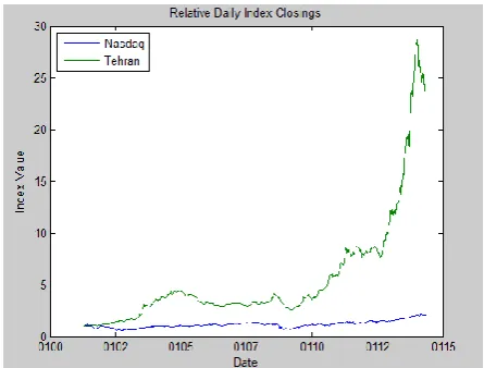
Fig. 1 illustrates the relative price movements of each Index. (Initial level of each Index has been normalized to unity to facilitate the comparison of their relative performances).
Fig. 1. Relative Price movements of each Index.
Since stock prices are mostly non-stationary, it is common in time series to model related changes of prices, that is the log return series. The log returns of the indices aredefined as:
= ln(
), = 1,2.
2
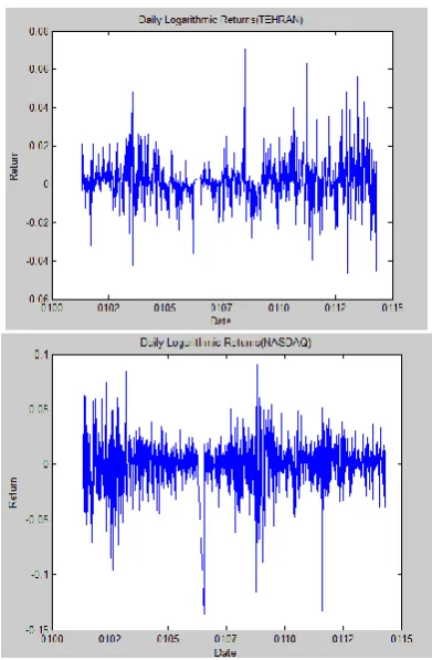
Where is the index price at time j;i=1,2 corresponding to stock index from TEHRAN STOCK EXCHANGE and NASDAQ, respectively. The market returns of TEHRAN SEand NASDAQ are shown in Fig. 2.
Fig. 2. Daily returns of TEPIX and NASDAQ
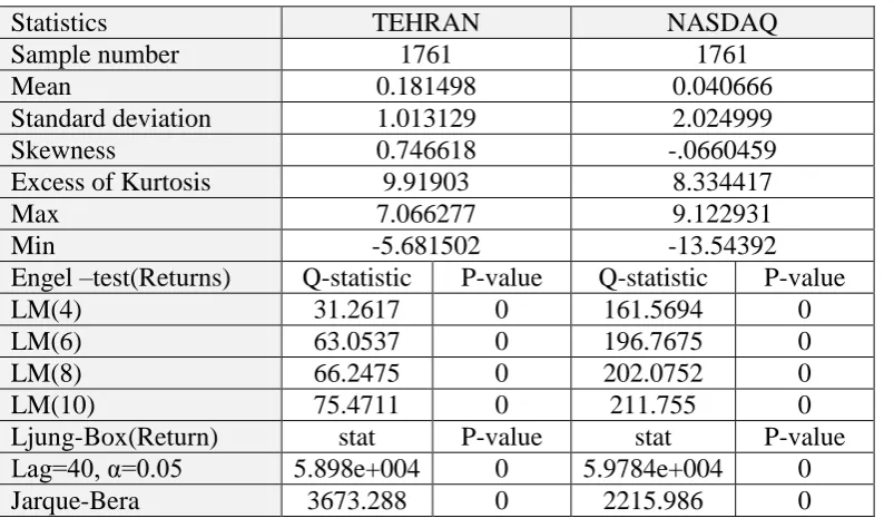
Table 1. Descriptive statistic and Engle tests.
Statistics TEHRAN NASDAQ
Sample number 1761 1761
Mean 0.181498 0.040666
Standard deviation 1.013129 2.024999
Skewness 0.746618 -.0660459
Excess of Kurtosis 9.91903 8.334417
Max 7.066277 9.122931
Min -5.681502 -13.54392
Engel –test(Returns) Q-statistic P-value Q-statistic P-value
LM(4) 31.2617 0 161.5694 0
LM(6) 63.0537 0 196.7675 0
LM(8) 66.2475 0 202.0752 0
LM(10) 75.4711 0 211.755 0
Ljung-Box(Return) stat P-value stat P-value
Lag=40, α=0.05 5.898e+004 0 5.9784e+004 0
Jarque-Bera 3673.288 0 2215.986 0
4.2. The marginal distribution & generalized Pareto distribution function to model the tail distribution
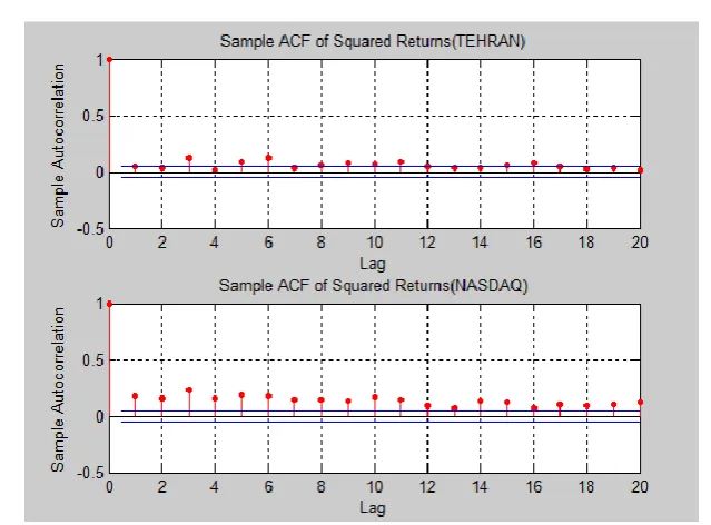
show that the Ljung-Box test applied to the residuals of the GARCH-n, GARCH-t , GJR-n and GJR-t models. Table 3 shows the results with values 1 meaning that the test rejects the null hypothesis at a 5% of significance level.
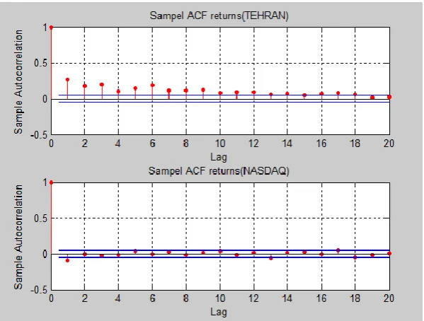
Fig. 3. Sample ACF of the Squared Returns.
Table 2. Estimation GARCH-GJR model and statistic test.
Mode l
GARCH-n GARCH-t GJR-n GJR-t
Index TEHRAN NASDA
Q TEHRA N NASDA Q TEHRA N NASDA Q TEHRA N NASDA Q
LLF 5.8
e+003 4.6e+00 3 6.1 e+003 4.7e+00 3 5.8 e+003 4.6e+00 3 6.1 e+003 4.7e+00 3
AIC
-1.15e+0 04 -9.2e+003 -1.2e+00 4 -9.4e+00 3 -1.1e+00 4 -9.2e+00 4 -1.2e+00 4 -9.4e+00 3
BLC
Table3. Estimation GARCH-GJR model and statistic test.
Mode l
GARCH-n GARCH-t
Index TEHRAN R
es
ult
NASDAQ R
es
ult
TEHRAN R
es
ult
NASDAQ R
es ult Ljung -Box Q-statisti c P-value Q-statisti c P-value Q-statisti c P-value Q-statisti c P-value QW(1 )
0.07.3 0.7909 0 0.0213 0.884 0 4.3869 0.036
2
1 0.0042 0.948
2
0
QW(3 )
0.317 0.9568 0 0.5474 0.66 0 10.946
5
0.12 1 1.9182 0.589
6
0
QW(5 )
0.3291 0.9971 0 4.0416 0.542
8
0 12.037
9
0.034 3
1 4.4519 0.486
3
0
QW(7 )
1.4583 0.9839 0 4.7421 0.991
4
0 20.338
5
0.004 9
1 5.1226 0.645 0
Engel -test Q-statisti c P-value Q-statisti c P-value Q-statisti c P-value Q-statisti c P-value LM(4 )
9.8528 0.043 1 1.3947 0.845
1
0 9.6627 0.046
5
1 0.6594 0.956
2 0 LM (6) 11.515 7
0.0737 0 1.4102 0.965
2
0 10.846
9
0.093 2
0 0.6969 0.994
6 0 LM (8) 13.152 9 0.1067 0
0 1.4522 0.995
5
0 12.743
5
0.121 0 0.7602 0.999
4 0 LM (10) 15.860 7
0.1037 0 2.2102 0.994
5
0 16.242
2
0.092 9
0 1.4668 0.999 0
Mode l
GJR-n GJR –t
Index TEHRAN R
es
ult
NASDAQ R
es
ult
TEHRAN R
es
ult
NASDAQ R
es ult Ljung -Box Q-statisti c P-value Q-statisti c P-value Q-statisti c P-value Q-statisti c P-value QW(1 )
0.0028 0.9579 0 0.0165 0.897
9
0 3.8472 0.049
8
1 0.0013 0.971 0
QW(3 )
0.0261 0.9989 0 1.617 0.655
5
0 12.618
3
0.005 5
1 2.2445 0.523
2
0
QW(5 )
0.0329 1 0 3.6062 0.607
4
0 13.471
8
0.019 3
1 4.5807 0.469
2
0
QW(7 )
0.4255 0.9997 0 4.2187 0.754
3
0 25.252 0.000
7
1 5.1816 0.637
8 0 Engel -test Q-statisti c P-value Q-statisti c P-value Q-statisti c P-value Q-statisti c P-value LM(4 )
9.0633 0.0595 0 1.8062 0.771
3
0 7.0254 0.134
6
0 0.8993 0.924
7 0 LM (6) 11.749 7
0.0678 0 1.8933 0.929
2
0 11.396 0.076
9
0 1.0177 0.984
9 0 LM (8) 12.524 6
0.1293 0 2.0371 0.979
9
0 11.778
6
0.161 4
0 1.2068 0.996
6 0 LM (10) 16.974 5
0.0749 0 3.0334 0.980
6
0 19.353
6
Given the standardized, i.i.d. residuals from the previous step, we estimate the empirical CDF of each index with a Gaussian kernel in interior and EVT in each tail, because the interior of a CDF is usually smooth, and non-parametric kernel estimates are well suited, but kernel smooth tends to perform poorly when applied to the upper and lower tails. To better estimate the tails of the distribution, we apply EVT to those residuals that fall in each tail.
4.3. Copula modeling
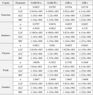
After having estimated the parameters of the marginal distribution , we continue to estimate the copula parameters as explained previously. Five copula functions are applied in our work: Gaussian copula, Student-t copula, and some Archimedean copula. According to the MLE and IFM methods, the selected copula functions will be fitted to these residuals series. The copula modeling result is showed in Table 4. Table 4 shows the results we estimate from the MLE or IFM method.
It is obvious to find the best fitting copula function we used the AIC and BIC criterion for model selection here. Table 4 shows that Clayton, Frank, Gumbel copulas AIC and BIC are the smallest, especially with the GARCH-t and GJR-t marginal distribution model.
Frank and Plackett's copulas, especially with the GARCH-t marginal distribution, which are a better fit than the Gaussian copula. In fact, the Gaussian copula with the GARCH-t marginal distribution model is the well-known distribution, which is the multivariate normal distribution we always assume in the classical method.
Table 4. Parameter estimates for families of copula and model selection statistic.
Copula Parameter GARCH-n GARCH-t GJR-n GJR-t
Gaussian
0.0822 0.0785 0.0764 0.0718
LLF 5.8163e+003 6.1003e+003 5.823e+003 6.114e+003 ALC -1.163e+004 -1.22e+004 -1.164e+004 -1.223e004 BIC -1.162e+004 -1.219e+004 -1.164e+004 -1.222e+004
Student-t
0.0707 0.0676 0.0655 0.0623
D 6.5010 6.0822 6.5095 6.129
LLF 5.1863e+003 6.1003e+003 5.823e+003 6.114e+003 ALC -1.163e+004 -1.22e+004 -1.164e+004 -1.222e+004
BIC -1.162e+004 -1.219e+004 -1.163e+004 -1.221e+004
Clayton
0.0821 0.081 0.0692 0.0643
LLF 5.8165e+003 6.1003e+003 5.8229e+003 6.1139e+003 ALC -1.163e+004 -1.22e+004 -1.164e+004 -1.223e+004 BIC -1.162e+004 -1.219e+004 -1.166e+004 -1.222e+004
Frank
.04058 0.3922 0.3782 0.3648
LLF 5.816e+003 6.1e+003 5.823e+003 6.114e+003 ALC -1.163e+004 -1.22e+004 -1.164e+004 -1.223e+004
BIC -1.162e+004 -1.219+004 -1.164e+004 -1.222e+004
Gumbel
1.0667 1.0649 1.0663 1.0668
LLF 5.8163e+003 6.1003e+003 5.823e+003 6.1139e+003 ALC -1.163e+004 -1.22e+004 -1.164e+004 -1.223e+004 BIC -1.162e+004 -1.219e+004 -1.164e+004 -1.222e+004
4.4. Estimation of VaR
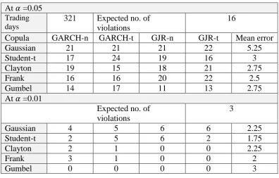
t = 2 to t = 1441 and estimate VaR 1443 by using observations t = 3 to t = 1442 until the sample-out observations we have updated are used up. Because we have 321 sample-out observations left, there are total 321 tests for VaR. The number of violations of the VaR estimation is calculated using various copula functions and are presented in Table 5.
The numbers of violations in Table 5 are the numbers of sample observations being located out of the critical value. The mean error shows for each copula function, the average absolute discrepancy per marginal model between the observed and expected number of violations. When the estimation of the number of violations calculated by various copula functions is closer to the expected number of violations (i.e., 16), the values of the mean error are small. From the results in Table 5, the Frank copula shows the minimum mean error with a 95% level of confidence and Student-t copula shows the minimum mean error with a 99% level of confidence. That is, the Frank copula is the best adequate copula for describing the return distribution of the portfolio.
Table 5. Number of violations of the VaR estimation.
At =0.05 Trading days
321 Expected no. of
violations
16
Copula GARCH-n GARCH-t GJR-n GJR-t Mean error
Gaussian 21 21 21 22 5.25
Student-t 17 24 19 16 3
Clayton 19 15 18 21 2.75
Frank 16 16 20 22 2.5
Gumbel 14 17 11 13 2.75
At =0.01
Expected no. of violations
3
Gaussian 4 5 6 6 2.25
Student-t 2 5 6 2 1.75
Clayton 2 1 0 0 2.25
Frank 3 1 0 0 2
Gumbel 0 0 0 0 3
Table 6. Number of violations of VaR estimation.
Trading days 321
5% 1%
Expected no. of violations 16 3 Mean error
Frank-copula- GARCH-n 16 3 0
Frank-copula- GARCH-t 16 1 2
t-copula- GARCH-n 17 2 2
t-copula- GJR-t 16 2 1
HS 5 1 13
5. Conclusion
This paper estimates different copulas with different univariate marginal distributions, and traditional methods to compare the results. The Frank copula describes the dependence structure of the portfolio return series quite well, in which we choose it by the AIC and BIC of the model criterion, producing the best results of the reliable VaR limit.
References
Jondeau, E. Rockinger, M, 2006. The copula-GARCH model of conditional dependencies: An international stock market application. Journal of International Money and Finance 25 (5), 827-853.
Ozun, A., Cifter, A., 2007. Portfolio value-at-risk with time-varying copula: Evidence from the Americans. Marmara University. MPRA Paper No. 2711. Thomas J. Linsmeier and Neil D. Pearson, 1996, "Risk Measurement: An Introduction to Value at Risk"
Patton, A. J. (2002). Modelling time-varying exchange rate dependence using the conditional copula. Working paper, UCSD.
Palaro, H., Hotta, L.K., 2006. Using conditional copulas to estimate value at risk. Journal of Data Science 4 (1), 93-115.
Jen-Jsung Huang, Kuo-Jung Lee, Hueimei Liang, Wei-Fu Lin, 2009, "Estimating value at risk"
Engle, R. F. and T. Bollerslev, 1986, "Modeling the persistence of conditional variances." Econometric Review 5:1–50.
Dias, A., and Embrechts, P. (2003). Dynamic copula models for multivariate high- frequency data in finance. Working Paper, ETH Zurich: Department of
Mathematics.
Embrechts, P. and Hoing, A., Juri, A. (2003). Using copula to bound the value-at-risk for functions of dependent value-at-risks. Finance and Stochastic 7, 145-167.
Embrechts, P., Lindskog, F. and McNeil, A.J. (2003). Modelling dependence with copulas and applications to risk management. In Handbook of Heavy Tailed Distributions in Finance (Edited by S. T. Rachev), 329-384 Elsevier
Wang Z R, Chen X H, Jin Y B and Zhou Y J (2009): '' Estimating risk of foreign exchange portfolio: Using VaR and CVaR based on GARCH-EVT-Copula model''. Physica A: Statistical Mechanics and its Applications 389 (21), 4918-4928.
Palaro, P. Hender, Hotta, K. Luiz, '' Using Conditional Copula to Estimate Value-at-Risk''. Journal of Data Science 4(2006), 93-115.
Ngoga Kirabo Bob (2013):''Value at Risk Estimation. A GARCH-EVT-Copula Approach''. Master thesis of Mathematic and Statistic, University of