Franck BOYER, Thierry GALLOUET, Rapha`ele HERBIN and Florence HUBERT Editors
COLLISIONS IN MAGNETISED PLASMAS
∗Philippe Ghendrih
1, Thomas Cartier-Michaud
1, Guilhem Dif-Pradalier
1,
Damien Esteve
1, Xavier Garbet
1, Virginie Grandgirard
1, Guillaume Latu
1,
Claudia Norscini
1and Yanick Sarazin
1Abstract. Approximations for closing the kinetic equation for the one particle distribution function are calculated by using propagators. These provide the formal structure of the collision term in the Landau approximation. The method allows one to investigate the effect of inhomogeneities at the Debye scale and to analyse magnetised collisions, when the Larmor radius is smaller than the Debye length. This method also allows one developing a simple renormalisation scheme to derive the Lenard-Balescu collision operator.
R´esum´e. Une m´ethode de propagateurs est utilis´ee pour fermer l’´equation cin´etique de la fonction de distribution `a une particule. Celle-ci donne acc`es `a la structure formelle de l’op´erateur de collision dans l’approximation de Landau. Elle permet alors de calculer l’effet d’inhomog´en´eit´e `a l’´echelle de la longueur de Debye et d’analyser les collisions magn´etis´ees, lorsque le rayon de Larmor est inf´erieur `
a la longueur de Debye. Cette m´ethode permet ´egalement de d´evelopper une m´ethode simple de renormalisation pour calculer l’op´erateur de collision de Lenard-Balescu.
Introduction
The physics of burning plasma that will be investigated experimentally in ITER [1] require a first principle simulation support to prepare and analyse the experiments. In particular simulations of the turbulent transport must be addressed to understand and monitor the confinement performance of the device. At the contem-plated density and thermal energy, the ITER plasmas will be characterised by a very small collisionality, in particular due to the plasma density. The latter is such that the typical distance between particles ranges from 10−6 m to 10−7 m. In this regime weak binary collisions are shown to prevail. One then benefits from these large inter-particle distances since they allow one to consider the collisions from a classical point of view and derive analytically first principle collision operators. The small collisionality of these plasmas leads to many unexpected features regarding plasma transport compared to neutral fluids. One of the most important is the requirement to address transport properties from the kinetic point of view.
In the present paper we review many known aspect of plasma collisions in Section 1. This allows one to introduce in a systematic fashion key aspects that will be used in the following Sections. In Section 2 we analyse the derivation of the kinetic equation for the one particle distribution function. Here we follow the 1987 ”Th`ese d’Etat” work [2] yet unpublished. The starting point is the Klimontovich density [3] but instead
∗ Philippe Ghendrih is most indebted to Radu Balescu, Jacques Misguich and Andr´e Samain who supervised his PhD work,
which has inspired many facets of the present work.
1 CEA/DSM/IRFM, Cadarache, 13108 Saint-Paul-Lez-Durance, France
c
EDP Sciences, SMAI 2015
of using the BBGKY expansion [3] we rather follow an averaging procedure, as proposed in [4], based on the ability of differentiating various states to determine a state probability that is assumed to be continuous. In Section 3, the derivation of the Landau collision operator is undertaken based on a quasilinear approach to calculate the correlation function of the fluctuating distribution functions of interacting particles. This provides an elegant formalism where the physical insight presented in Section 1is used as a guideline. The step to the Lenard-Balescu collision operator is then straightforward by further expanding the correlation function and the propagator formalism, Section3. A simple renormalisation scheme then allows one to sum-up the contributions that readily appear as an expansion of the plasma permittivity. The issue of distribution function gradients at the Debye scale is addressed in Section 4 together with the collision operator for magnetised plasmas. The latter issue is more developed in [2] but requires to be revisited in the framework of modern gyrokinetics [5] and for optimum application for gyrokinetic codes such as the GYSELA code [6]. Finally the conservation laws are addressed together with the entropy production due to the collision operator, Section5. A short conclusion closes the paper.
1.
Collisions and particle trajectories in magnetised plasmas
1.1.
Gyration motion in the magnetic field
The key aspect of magnetic confinement is the charged particle gyration motion in the magnetic field. The Newton law for such a motion is:
ma
dv
dt =qav×B. (1)
where ma, qa are the mass and charge respectively of the particle of speciesa. This equation is homogeneous
with respect to the velocity v and exhibits the characteristic time ma/(qaB) = 1/Ωa, hence the inverse of
the Larmor gyration frequency Ωa, which depends on the magnitude of the magnetic field. For ions with
qa/ma≈e/mp≈108 C / kg,eis the unit charge andmp the proton mass, one then finds that Ωa≈5.108 s−1
for the magnetic field foreseen on ITER,B ≈5 T. In fusion plasmas, the Larmor period 1/Ωa is a very small
and shorter than most time scales of interest which allows one to introduce a time scale separation.
The gyration motion characterised by Eq.(1) exhibits two symmetries, first v ·v˙ = 0, which ensures the conservation of the kinetic energy proportional to v2, second, for a constant magnetic field in space and time,
B·v˙ = 0, which yields that the velocity component parallel to the magnetic field is constant, vk(t) =vk(t0) at all times. As a consequence, of these two first relations, one also has te conservation ofv⊥2 wherev⊥ is the
modulus of the velocity component transverse to the magnetic field.
One can notice from Eq.(1) that one can readily obtain a first integral of this equation:
ma
dx
dt =qa
x−xG
×B+mavk(t0)B/B, (2)
where xG andvk(t0) are the three integration constants. In such an expression the positionxG is that of the
cylindrical symmetry axis of the particle motion, the latter being aligned with b = B/B. Considering the transverse motion with velocityv⊥ and Larmor radiusρ=x−xG, one thus obtains:
v⊥=ρ×Ωa ; ρ=b×
v⊥
Ωa
; Ωa=
qa
ma
B. (3)
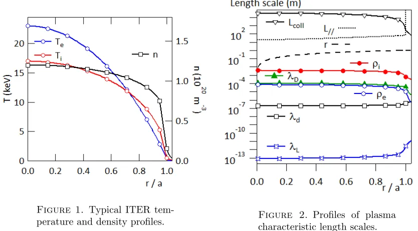
Figure 1. Typical ITER
tem-perature and density profiles. Figure 2.characteristic length scales.Profiles of plasma
magnetic field to the charged particles is at lowest order characterised by a cylindrical symmetry.
In order to illustrate the order of magnitude of the various scales introduced in this paper, we consider ITER [7] characteristic profiles for the ion and electron temperature as well as the density fig.(1). The ITER tokamak has a toroidal geometry with major radius R = 6 m and minor radius a = 2 m. On the profiles, one readily identifies three regions: the core plasma extending typically from r/a = 0 to r/a = 0.95, the pedestal region with sharp gradients fromr/a= 0.95 to r/a= 1, and the SOL region withr/a≥1 which is a thin boundary layer where the temperature profiles and the density decay exponentially to zero. Given ITER temperature characteristic profiles fig.(1), one can determine that of the Larmor radius, fig.(2), for the ions (closed circles) and for the electrons (open circles). These transverse scales are much smaller than the minor radius of the plasma, r (dashed line), fig.(2).
1.2.
Maxwell equations: charge conservation, charge screening
Starting from the Maxwell equations and introducing the electric and vector potential allows one to split this set of equations into geometrical features that determine the relationship between the electromagnetic field and the electromagnetic potential on the one hand and to equations governing the source terms, space charge and currents for the electromagnetic field on the other hand.
∇·B= 0 ; B=∇×A, (4)
∇×E=−∂
∂tB ; E=−∇U− ∂
∂tA, (5)
∇·E= ρ 0
; ∂
c ∂t ∂
c ∂tU−∇
2U= ρ
0
, (6)
∇×B=µ0j+
∂
c2 ∂tE ;
∂ c ∂t
∂
c ∂tA−∇
2A=µ
Accordingly, the definition of the potentials is completed by the Lorenz gauge:
c∇·A+ ∂
c ∂tU = 0. (8)
Combining the Maxwell equation relating the electromagnetic potentials,U andA, to charge densityρEq.(6) and current density j Eq.(7) and the Lorenz gauge Eq.(8), one readily recovers the fundamental charge conservation equation:
∂
∂tρ+∇·j= 0. (9)
The latter readily stipulates that if no current is flowing out of a given volume the charge density within that volume is the initial one, hence that charge neutrality in that volume is conserved. This is a general form of the quasi-neutrality equation since it postulates that at a given scale, so that the electric current vanishes, the system appears as neutral. Normalising the time space scales with τ and L and introducing U∗ =e U / T¯, A∗ =A L /B¯,ρ∗ =ρ/(e ¯n) andj∗ =j LB/¯ (¯nT¯) where ¯nand ¯T are the characteristic particle density and temperature of the plasma respectively andeis the electric charge. The normalising current is defined in terms of the normalised magnetic field having in mind the MHD force balance between the pressure gradient and the Laplace forcej×B. One then obtains:
L
c τ 2τ ∂
∂t τ ∂ ∂tU
∗−
L∇2U∗=e 2 n L¯ 2
0 T¯
ρ∗ =
L
λD
2
ρ∗, (10)
L
c τ 2τ ∂
∂t τ ∂
∂tA
∗−L∇2A∗= n¯ T¯
¯ B2/ µ
0
j∗ = β j∗, (11)
L∇·A∗ = −
D
B
τ c2 τ ∂
c ∂tU
∗. (12)
The right-hand side of this set of equations exhibits three dimensionless parameters that depend on well known plasma parameters. The Debye scale λ2
D =0 T /(e2n) is a measure of the importance of charge separation at scaleL in generating the electromagnetic field Eq.(10). One thus finds that at large scales, very small charge densities associated to polarisation effects generate the electromagnetic fields. The plasma is then considered as quasineutral, ρ≈n(λD/L)2. Consequently, with L λD, one finds the quasineutrality condition ρ→0.
Regarding Eq.(11), the dimensionless parameter is the MHDβ parameter which characterises the generation of magnetic fields by the plasma. In Eq.(12), one finds the Bohm diffusion coefficient DB =e T / B, and
therefore the departure from the Coulomb gauge ∇·A= 0. The condition can also be expressed in terms of the Larmor radius and frequency Eq.(3), asDB/(τ c2) =
ρ2/(cτ)2)(Ωτ). This parameter tends to zero in most cases of interest in plasma physics.
The profile of the Debye scale for ITER typical parameters is plotted on fig.(2) (closed triangles). One finds that λD ≥ ρe, hence that regarding the electrons, the Coulomb interactions close to the screening limit are
magnetised. This feature is also clear on fig.(4) where the ratioλD/ρeis larger than unity over the whole profile
and increases sharply in the SOL region.
1.3.
Coulomb collision mean free path
Various scales characterise the collisions. First one can introduce the Landau scaleλL such that the kinetic
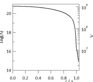
Figure 3. Profiles of the ratios of plasma characteristic length scales.
Figure 4. Plasma parameter profile.
is given by the thermal energyT. The Landau scale is therefore defined as:
T λL=
e2 4π0
=α ; λ3d n= 1. (13)
In burning plasmas, this scale is such that λL ≤10−13 m so that a sufficiently large number of fusion events
occur. This threshold effect is equivalent to the threshold on the plasma thermal energyT ≥10keV. The con-stantα=e2/(4πε0) will be used in the following to simplify the notations. Another relevant scale is the typical distance between the particles, the Loschmidt scaleλd Eq.(13). In all magnetic fusion plasmasλL/λd1, see
fig.(3). This means that the average kinetic energy of the particles, the thermal energy, is always much larger than the typical Coulomb potential energy. The collisions are therefore a weak effect and particles are mostly free-streaming and only constrained by the electromagnetic field, in particular the large magnetic field.
GivenλL andλd one can readily estimate the Debye length Eq.(10).
λD=
0T
e2n 1/2
=λd
1 2√π
λ
d
λL
1/2
. (14)
One thus finds λD λd when λd λL, which means that the screening effect at the Debye scale occurs in
regions of very small interaction energy via the collisions compared to the kinetic energy.
When analysing the effect of weak binary collisions, one finds that the most important effect is the change in direction of the relative velocity of the interacting particles during the collision, the deflection angleεb. One
can expect this angle to depend on the impact parameter b, see figure (5). The deflection of the trajectory of a given particle is a random function with positive and negative deflection events. On average one thus finds
εb
= 0 and therefore that the deflection angles exhibits a diffusive process. The collision mean free pathLcoll
interaction, hence a deflection of the order of π, hence:
Z
db 2π b Lcolln
ε2b
π2 ≈1. (15)
The key parameter to determine the collision mean free path is therefore the typical deflection angle during a binary collision. In the following we will calculate this angle, first in a simplified way that underlines the key aspects of weak Coulomb collisions and with an exact calculation. However, before proceeding to the calculation, one can estimate εb =λL/b from a simple dimensional point of view, retaining the fact that the
larger the impact parameter, the smaller the deflection. With this approximation one readily obtains:
Lcoll≈
π 2
λ3d λ2
L
Z db
b −1
=λd
π 2
λd
λL
2 1
Log(Λ). (16)
In typical systems with neutral particles, the collision mean free path is comparable to the Loschmidt scale. However, in plasmas this distance is much larger due to the parameter (λL/λd)−2, fig.(3). The effect of the
Coulomb logarithm Log(Λ) stemming from the integration over the impact parameterb does not balance the former effect, fig(4).
The cut-off introduced to bound the logarithmic divergence of the integrated Coulomb potential energy is twofold, towards the smallest scale the Landau scale separates the weak and strong collisions is thus sets a lower bound. Towards the largest scales, the Debye scale λD is an upper bound governed by the screening
properties. The Coulomb logarithmLog(Λ) depends on the plasma parameter Λ, which is then defined by the chosen cut-offs:
Λ = λD λd
λd
λL
= 1 2√π
λ
d
λL
3/2
= 4π λ3Dn. (17)
One thus readily finds that the plasma parameter Λ is a large number, large enough to yield a Coulomb loga-rithmLog(Λ) exceeding 10, fig(4) .
Regarding the strong binary collisions, one can readily estimate the mean free path associated to this effect by considering that all collisions in the volumeπλ2L LScoll to be large, hence given the density:
LScoll≈λd
1 π
λ2
d
λ2
L
=Lcoll
2
π2 Log(Λ)
. (18)
The Coulomb logarithm set the ratio between the two collision mean free paths, LScoll Lcoll provided that
Log(Λ)1. Given this condition, one can then work in the approximation of weak binary collisions.
1.4.
Weak Coulomb collisions
Let us consider the calculation of the deflection angle due to weak Coulomb collisions considering two charged particles labelled 1 and 2. We separate the system in the motion of the mass centre and the relative motion. For isolated binary collisions, the momentum of the mass centre is conserved and one can thus concentrate on the relative motion with the reduced massm=m1m2/M, whereM =m1 +m2and the central forceq1q2αrˆ/r2 where 4π0α=e2,qi=ei/eis the normalised charge of particleiof chargeei. The distance to the mass centre
israndˆris the unit vector from the mass centre to the relative particle position. The plane where the collision deflection takes plane is then defined by the origin, the mass centre, the vector rˆand the relative velocity v
of the deflection so that the relative velocity at t → −∞ is oriented along the y-axis, v =−v∞ yˆand such
that the particle reaches the x-axis, y = 0, at time t = 0. We further introduce the impact parameter b as the distance between the knock on axis (b=0) and the parallel axis defined by the position and velocity of the particle att→ −∞, see fig.(5).
In the simplified approach, we consider that the motion along they-axis is unperturbed so thaty=v∞t at
all times. The deflection will then be determined by the momentum transfer along xcompared to mv∞ and
thus determined by the integration of the Coulomb force projected onxfrom t→ −∞tot→+∞, hence:
εb(t) =
∆(m vx)
mv∞
= 2 Z t
0
dt0 q1 q2α r2 = 2
2q1 q2 α
m v2
∞b
Z tv∞/b
0
du 1 (1 +u2)3/2 =
λL
b
t v∞/b
1 + (t v∞/b)2
1/2. (19)
At the limitt→+∞, one thus recovers the expression used in Section (1.3), the trajectory during the collision remaining unaffected in the y-direction. This model also allows one to determine where most of the deflection
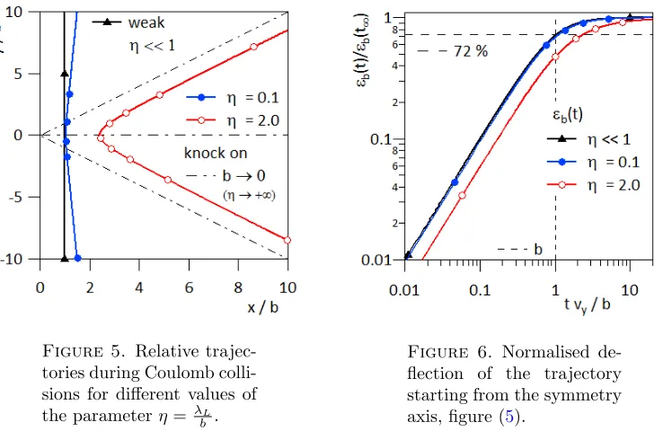
Figure 5. Relative trajec-tories during Coulomb colli-sions for different values of the parameterη= λL
b .
Figure 6. Normalised de-flection of the trajectory starting from the symmetry axis, figure (5).
occurs, fig.(6). One finds that within this approximation, labelled by η 1 in fig.(6), more than 70 % of the deflection occurs at a distance equal to the impact parameter from the mass centre. Hence, during a typical collision at the Loschmidt scale, the binary interaction is predominantly governed by one neighbouring particle.
The complete model for the Rutherford collision is readily derived from the angular momentum Eq.(20) and energy Eq.(21) conservation laws. In cylindrical coordinates (r, θ), this yields:
dτ
dθ = u
−2, (20)
dθ
du = −
1
1−η u−u2 1/2
whereu=b/r,bis the impact parameter,τis the normalised time,τ =v∞t/bandη=λL/b. Changing variable
in the second equation with z= (u+η/2)/(1 +η2/4)0.5 andz= cos(θ), hence:
cos(θ) = u+η/2
(1 +η2/4)1/2 . (22)
Given the chosen symmetry, see fig.(5), one obtains the minimum value ofr atθ= 0. The deflection angle b
is then determined by:
sin(b) =sin(2θ∞) =
η
1 +η2/4. (23)
One thus recovers b = η = λL/b as used for the calculation of the mean free path. The deflection angle
computed here is that of the relative motion. It must be multiplied by a mass ratio to determine the actual deflection for the particles. For like-particles collisions or for electrons impacting ions this does not change the order of magnitude. However for ions impacting electrons this has a large impact by reducing the deflection angle according to the mass ratiome/mi.
2.
Kinetic equation
2.1.
Klimontovich density and Liouville probability
We follow here a standard approach [3] starting from the Klimontovich densityFa(Z, t) for speciesaat point
Z = (X,P) of the phase space and at time t.
Fa(Z, t) =
X
ia
δZ−Zia(t)
=X
ia
δX−Xia(t)
δP−Pia(t)
. (24)
The Klimontovich densityFa(Z, t) accounts for point particles labelled byia. The trajectory for a given particle
in phase space is thus defined byZia(t) =
Xia(t),Pia(t)
and is determined by the HamiltonianH such that:
dXia
dt =
∂H
∂Pia
=−[H,Xia]X,P, (25)
dPia
dt = −
∂H
∂Xia
=−[H,Pia]X,P, (26)
where the Hamiltonian is the sum of the contribution of each kinetic energy and of the interaction coulomb potentials.
H=X
a
X
ia
H 0
a+
1 2
X
b
X
jb
α qaqb
|Xia−Xjb|
= X
a
X
ia
Ha(Zia, t). (27)
The Coulomb interaction potential only depends on the distance between particles in physical space |rij| =
|Xi−Xj|. The summation over aand b are summations over species and the summation over ia andjb are
summations over the particles of a given speciesaandb respectively. The massma and charge number Za are
only species dependent, hence labelled by a for species a, withqa = ea/|e| ea being the charge of species a.
The interaction constant of the Coulomb potential is α=e2/(4πε0). Note that for identical particles, hence identical species and identical particle label, one has |rij|= 0, however the divergence is removed because the
interaction potential between a particle and itself is equal to zero. Implicitly one thus assumes that only one par-ticle can be located at a given location in physical spaceX. The HamiltonianH0
The phase space integration of the Klimontovich density for speciesayields the number of particles of species a,Na. The phase space integral accounts for the whole space inP and a volumeV for the physical space.
Z
dZFa(Z, t) =
Z dX
Z
dP Fa(Z, t) =Na. (28)
Assuming that particles are not created nor destroyed, one can then consider the particle conservation equation, which yields:
dFa(Z, t)
dt =
∂Fa(Z, t)
∂t − h
HFa(Z, t)
i
X,P = 0. (29)
The Poisson brackets are defined as:
h F, Gi
X,P
= ∂F ∂X ·
∂G ∂P −
∂G ∂X ·
∂F
∂P. (30)
The subscript X, P in the Poisson bracket specifies which variables are used and the order of the derivatives. It will be dropped at a later stage to simplify the notation. The extension of the Liouville equation Eq.(29) to a case with particle creation or destruction can readily be done by implementing a non vanishing right-hand side, yielding the creation/destruction rate.
Introducing the definition Eq.(24) in Eq.(29), one obtains:
∂Fa(Z, t)
∂t + X
ia
˙ Xia·
∂Fa(Z, t)
∂Xia
+P˙ia·
∂Fa(Z, t)
∂Pia
= 0. (31)
Given the definition of the Klimontovich density in terms ofδfunctions, one then readily obtains:
∂Fa(Z, t)
∂t +
˙
X·∂Fa(Z, t)
∂X + ˙
P ·∂Fa(Z, t)
∂P
= ∂Fa(Z, t) ∂t −
h H, Zi
X,P ·
∂Fa(Z, t)
∂Z = 0. (32)
In this result, the two fieldsX˙ andP˙ are extended to regions where particles are not necessarily located. Let us now introduce the Liouville probabilityPL
{zi}, t
for a elementary-state where particleiis located
in phase space numberixi,pi
at (Xi(t),Pi(t)) =Zi(t) at timet, and similarly for all particles. Each particle
is then located in its own specific 6D phase space. Note that for the Liouville probability the species index is dropped because this probability encompasses all particles and species of the plasma in defining elementary-state for the whole plasma in the volumeV. Using a Hartree-Fock structure, hence multiplicative probabilities as for independent events, one then defines the probability of the given elementary-state as:
PL
{zi}, t
= Y
a, ia
δzi−Zia(t)
= Y
a, ia
δxi−Xia(t)
δpi−Pia(t)
, (33)
where {zi} is the coordinate ensemble for all species in theN = PaN a phase-spaces of dimension 6D. As
defined in Eq.(33), the Liouville is the probability to have particle i located at the chosen position zi and
range. Such a micro-state is then the mean of all the elementary-states of the form (33) that yield the same
electromagnetic field. The probability for the micro-state is then PL
{zi}, t
=<PL
{zi}, t
>µstate that we
enforce to be continuous in phase space [8]. This procedure thus allows one to avoid the BBGKY hierarchy to directly address the physics of the one particle distribution function. When addressing the collisions, the equation for the two particle distribution function is then built starting from the one particle distribution. This leads to developing an inverse BBGKY hierarchy, where only the two first equations are relevant to address the collisions in fusion plasmas. More mathematical settings of such a procedure exist, for example [9]. However such works remain within the BBGKY standard framework. One then defines the one particle distribution function of speciesaas the average Klimontovich density for speciesawhere the weight in the averaging process is the Liouville probability of the micro-state. This Liouville average can also be seen as the projection of PL on
Fa(Z, t).
Fa(Z, t) = Na
Y
ia=1
Z
dziaFa(Z, t)
Y
b, ib
Z dzibP
{zi}, t
=hFa(Z, t)iPL. (34)
2.2.
Average and fluctuation separation with the Liouville average
Given the Liouville average defined in Eq.(34), one can separate the Klimontovich density as the sum of its averageFa(Z, t) and fluctuating partsfa(Z, t), hence:
Fa(Z, t) =Fa(Z, t) +fa(Z, t). (35)
Dropping the subscript X, P in the Poisson bracket, the kinetic equation Eq.(31) can then be written as the evolution of the mean and fluctuating parts of the Klimontovich density:
∂Fa(Z, t) +fa(Z, t)
∂t −
h
H+h, Fa(Z, t) +fa(Z, t)
i
= 0. (36)
In this equation we also separate the Hamiltonian into its mean and fluctuating part so that: H=H+h. The equation can then be split into the mean equation obtained by averaging Eq.(36):
∂Fa(Z, t)
∂t − h
H, Fa(Z, t)
i
−Dhh, fa(Z, t)
iE
PL
= 0, (37)
and the fluctuation part which is the obtained by subtracting Eq.(37) from Eq.(36).
∂fa(Z, t)
∂t − h
H, fa(Z, t)
i
−hh, Fa(Z, t)
i −
h
h, fa(Z, t)
i
−Dhh, fa(Z, t)
iE
PL
= 0. (38)
These steps are standard in all quasilinear approaches. Regarding collisions, one can replaces H and h by a more explicit dependence on the Coulomb potential starting from Eq.(27)
Ha(Zia, t) = H
0
a(Zia, t) +
X
b
X
jb
α qaqb
|Xia−Xb|
δXb−Xjb
= Ha0(Zia, t) +
X
b
α qaqb
|Xia−Xb|
X
jb
δZb−Zjb(t)
. (39)
This expression thus depends explicitly on the Klimontovich densityFb(Zb, t)
Ha(Za, t) =Ha0(Za, t) +
X
b
Z dZb
α qaqb
|Xa−Xb|
so that:
Ha(Za, t) = Ha0(Za, t) +
X
b
Z dZb
α qa qb
|Xa−Xb|
Fb(Zb, t), (41)
ha(Za, t) =
X
b
Z dZb
α qa qb
|Xa−Xb|
fb(Zb, t). (42)
These expressions then lead to:
∂Fa(Za, t)
∂t − h
Ha(Za, t), Fa(Za, t)
i −X
b
∂
∂Pa
· Z
dZb
∂
∂Xa
α q
a qb
|Xa−Xb|
fb(Zb, t)fa(Za, t)
PL
= 0. (43)
The source term in the evolution of the distribution function is the third term of Eq.(43) which explicitly depends on the correlation functionCa,b(Za, Zb, t) =< fa(Za, t)fb(Zb, t)>PL.
∂Fa(Za, t)
∂t − h
Ha(Za, t), Fa(Za, t)
i − ∂
∂Pa
·X
b
Z dZb
∂
∂Xa
α q
a qb
|Xa−Xb|
Ca,b(Za, Zb, t) = 0. (44)
The next steps in the calculation of the collision operator then aims at reducing the correlation function Ca,b(Za, Zb, t) to a function of the single particle distribution functions so that one obtains an equation of
the form Eq.(44) that only depends of the distribution function, thus closing the kinetic equation of the one particle distribution function.
3.
Collision operators: expanding the correlation function
3.1.
Expansion of the correlation function in terms of the one-particle and two-particle
distribution functions
The correlation functionCa,b is related to the Klimontovich densities:
Ca,b(Za, Zb, t) =hFa(Za, t)Fb(Zb, t)iP−Fa(Za, t)Fb(Zb, t). (45)
The correlation function of the two Klimontovich densities is split into two contributions of different orders. First, fora=bandZa=Zb one obtains the self correlation term equal to the one particle distribution function.
The contribution for different species,a6=b, or for different particles of the same species,a=bandZa6=Zb, is
by definition the two-particle distribution function that can be expanded asFa(Za, t)Fb(Zb, t) +ga,b(Za, Zb, t).
One thus obtains:
Ca,b(Za, Zb, t) =δ(a, b)δ(Za−Zb)Fa(Za, t) +ga,b(Za, Zb, t). (46)
In Eq.(44), the self-correlation term does not contribute since it leads to self-Coulomb interaction which is set to zero. The lowest order contribution of the correlation function then yields the Vlasov equation. One must therefore determine the higher order contribution, ga,b(Za, Zb, t) to obtain a non-vanishing collision operator.
∂Fa(Za, t)
∂t − h
Ha(Za, t), Fa(Za, t)
i − ∂
∂Pa
·X
b
Z dZb
∂
∂Xa
α q
a qb
|Xa−Xb|
3.1.1. Formal solution for the fluctuations of the Klimontovich density
Given the definition of the correlation functionCa,b(Za, Zb, t), one can either solve Eq.(38) to determine the
evolution of the fluctuating densities fa andfb or address the evolution of the correlation function. Formally,
Eq.(38), can be written as:
∂tfa(Za, t) +La(t)fa(Za, t) =Ka(t)Fa(Za, t). (48)
The evolution offathen depends on two contributions, a source term via the operatorKathat explicitly depends
on the fluctuating part of the Hamiltonian acting on the one-particle distribution function, and a contribution that only depends on the fluctuating part of the Klimontovich density. The solution of Eq.(48) can be written as:
fa(Za, t)−Λ(t, t0)fa(Za, t0) = Z t
t0
dt0∂t0
Λa(t, t0)fa(Za, t0)
=
Z t
t0
dt0Λa(t, t0)Ka(t0)Fa(Za, t0), (49)
where the propagator Λa(t, t0) is defined by:
∂tΛa(t, t0) =−La(t)Λa(t, t0). (50)
The fluctuating particle densityfa then depends on two terms, the propagation with Λa of the fluctuations at
timet0and the generation and propagation of fluctuations due to the source term, therefore:
fa(Za, t) = Λa(t, t0)fa(Za, t0) + Z t
t0
dt0Λa(t, t0)Ka(t0)Fa(Za, t0). (51)
3.1.2. Formal solution for the correlation function of Klimontovich density fluctuations
For convenience we note this solution as fa = pa+sa, the propagation on initial fluctuations pa and the
generation part due to the sourcesa. With this notation the correlation function for different species, or different
particles of the same species,Ca,b(Za, Zb, t) =ga,b(Za, Zb, t) takes the form:
ga,b(Za, Zb, t) =
D
papb+ (pasb+pbsa) +sasb
E
P
. (52)
In order to maintain the explicit symmetry between speciesaandbin the calculation, we use the operatorPa,b,
which permutes speciesaandb, hence:
ga,b(Za, Zb, t) =
I+Pa,b
2
papb+sasb
+I+Pa,b
sapb
P
. (53)
Using the two forms for the source term Eq.(49) one then obtains:
I+Pa,b
2 sasb=
I+Pa,b
2
Z t
t0
dt0Λa(t, t0)Ka(t0)Fa(Za, t0)
Z t
t0
dt00∂t00
Λb(t, t00)fb(Zb, t00)
. (54)
Given the symmetry that is enforced by the operatorI+Pa,bbetween the two integrals, one can order the time
integrals so that:
I+Pa,b
2 sasb=
I+Pa,b
Z t
t0
dt0Λa(t, t0)Ka(t0)Fa(Za, t0)
Z t0
t0
dt00∂t00
Λb(t, t00)fb(Zb, t00)
which then yields:
I+Pa,b
2 sasb =
I+Pa,b
Z t
t0
dt0Λa(t, t0)Ka(t0)Fa(Za, t0)
Λb(t, t0)fb(Zb, t0)−Λb(t, t0)fb(Zb, t0)
= I+Pa,b
Z t
t0
dt0Λa(t, t0)Λb(t, t0)Ka(t0)fb(Zb, t0)Fa(Za, t0)−
I+Pa,b
sapb. (56)
Similarly to the fluctuating particle density Eq.(51), one obtains the correlation function as the sum of two terms: one determined by the evolution of initial fluctuations and the other related to the evolution of fluctua-tions generated by the collisions that act as a source term.
ga,b(Za, Zb, t) = I
+Pa,b
2 D
Λa(t, t0)fa(Za, t0)Λb(t, t0)fb(Zb, t0) E
P
+I+Pa,b
Z t
t0
dt0DΛa(t, t0)Λb(t, t0)Ka(t0)fb(Zb, t0)
E
PFa(Za, t
0). (57)
It is to be noted that the evolution operator Λ also depends on the fluctuations and therefore does not commute with the averaging procedure.
3.1.3. Self-similarity of the correlation function
Let us now consider the two operators Ka(t0) and Λ(t, t0) defined by Eq.(48) and Eq.(38) together with
Eq.(50). One then obtains:
Ka(t)Fa(Za, t) =
h
h, Fa(Za, t)
i =X
c
Z dZc
∂
∂Xa
α qa qc
|Xa−Xc|
fc(Zc, t)·
∂
∂Pa
Fa(Z, t), (58)
Lafa(Z, t) =
h
H, fa(Za, t)
i
+hh, fa(Za, t)
i
−Dhh, fa(Za, t)
iE
P
. (59)
Both operators depend on the fluctuations. The operatorKa directly describes the binary interaction between
the particles of the Klimontovich density. This is the source of the fluctuations in the present description. Conversely the operatorLadepends on the fluctuations only via a second order impact on the particle trajectories
and therefore on the evolution of the Klimontovich density. We concentrate here on the lowest order effect, namely the source of the fluctuations via the binary interactions. We thus consider the evolution operator L0
a
and the associated propagator Ua(t, t0) such that:
L(0)a fa(Z, t) = −
h
H, fa(Z, t)
i
, (60)
∂tUa(t, t0) = −L(0)a Ua(t, t0). (61)
With this approximation one then obtains:
ga,b(Za, Zb, t) =
I+Pa,b
2
Ua(t, t0)Ub(t, t0) D
fa(Za, t0)fb(Zb, t0) E
P
+I+Pa,b
Z t
t0
dt0Ua(t, t0)Ub(t, t0)
X
c
Z dZc
∂
∂X
α qa qc
|Xa−Xc|
· ∂
∂Pa
Fa(Za, t0)
D
fc(Zc, t)fb(Zb, t0)
E
and therefore:
ga,b(Za, Zb, t) =
I+Pa,b
2
Ua(t, t0)Ub(t, t0)Ca,b(Za, Zb, t0)
+I+Pa,b
Z t
t0
dt0Ua(t, t0)Ub(t, t0)
X
c
Z
dZc qaqcRa(Za, Zc, t0)Fa(Za, t0)Cc,b(Zc, Zb, t0).(63)
Where we have now introduced the operatorRa(Za, Zc, t) such that:
Ra(Za, Zc, t)Fa(Za, t) =
∂
∂Xa
α
|Xa−Xc|
· ∂
∂Pa
Fa(Za, t). (64)
We thus find that the correlation function depends on the correlation function at previous times in a self-similar fashion with two contributions, the free evolution of the initial correlations att=t0, first term on the right hand side of Eq.(63) and the creation via binary interaction and subsequent free evolution of correlations, second term on the right hand side of Eq.(63).
Following Bogoliubov, we consider a scale separation in time, assuming that the characteristic time of the correlations is much shorter than the characteristic evolution time of the one particle distribution function, typicallyt−t0in Eq.(57). We can then neglect the evolution of the initial fluctuations that will have died away long before the reference timet.
ga,b(Za, Zb, t) =
I+Pa,b
Z t
t0
dt0Ua(t, t0)Ub(t, t0)
X
c
Z
dZc qaqcRa(Za, Zc, t0)Fa(Za, t0)Cc,b(Zc, Zb, t0).(65)
In this expression one can notice the development of a collective behaviour via the summation on the speciesc as well as the dependence on previous timest0.
3.2.
Landau collision term
Given the self-similar form of the correlation function Eq.(65) and the dependence of the correlation function on the one and two particle distribution functions Eq.(46), one obtains:
ga,b(Za, Zb, t) = qa qb
I+Pa,b
Z t
t0
dt0Ua(t, t0)Ub(t, t0)Ra(Za, Zb, t0)Ua(t0, t)Ub(t0, t)Fa(Za, t)Fb(Zb, t)
+I+Pa,b
Z t
t0
dt0Ua(t, t0)Ub(t, t0)
X
c
Z
dZc qaqcRa(Za, Zc, t0)Fa(Za, t0)gc,b(Zc, Zb, t0).(66)
In this expression we have introduced the inverse operators Ua(t, t0)−1 = Ua(t0, t) and Ub(t, t0)−1 = Ub(t0, t)
in the lowest order contribution to the right and side. In order to address the structure of the kernel of this contribution let us use the expression of the operatorRa Eq.(64) in terms of its Fourier transform in space.
Ra(Za, Zb, t0)Fa(Za, t0) =
Z
dKeiK·(Xa−Xb) q
a qb V(K)iK·
∂
∂Pa
Fa(Za, t0). (67)
The kernel is then given by:
Ua(t, t0)Ub(t, t0)Ra(Za, Zb, t0)Ua(t0, t)Ub(t0, t)
= Z
dK Ua(t, t0)Ub(t, t0)eiK·(Xa−Xb)Ua(t0, t)Ub(t0, t)qa qb V(K)iK·
∂
∂Pa
When considering the free streaming approximation for the propagatorUa, one has:
Ua(t, t0) = exp
−(t−t0)va·∇a
, (69)
depending on the velocity v =P/mand where∇a is the compact form of the derivative with respect to the
position is spaceXa:
∇a=
∂
∂Xa
. (70)
The calculation of the kernel of the operator is then straightforward and yields:
Ua(t, t0)Ub(t, t0)Ra(Za, Zb, t0)Ua(t0, t)Ub(t0, t)
= Z
dK expiK·(Xa−Xb−(t−t0)va,b)
qa qb V(K)iK·
∂
∂Pa
, (71)
wherevab=va−vb is the relative velocity.
The lowest non-vanishing collision operator, the Landau collision operator, is then determined by the corre-lation function:
ga,b(1)(Za, Zb, t) =
I+Pa,b
Z t
t0
dt0 Z
dK expiK·(Xa−Xb−(t−t0)vab)
qa qb V(K)Fb(Zb, t)iK·
∂
∂Pa
Fa(Za, t), (72)
which then yields:
Ca
Fa(Za, t)
= − ∂
∂Pa
·X
b
Z dZb
Z
dK0 K0expiK0·(Xa−Xb)
qa qb V(K0)
I+Pa,b
Z t
t0
dt0 Z
dK expiK·(Xa−Xb−(t−t0)vab)
qa qb V(K)Fb(Zb, t)K·
∂
∂Pa
Fa(Za, t). (73)
To recover the standard form of the collision operator, we introduce another scale separation such that the scale of variation of the one particle distribution function is much larger than the relative distance between the particle during the binary interactionXab=Xa−Xb. The integration overdXb then leads toK=−K0 with
the ordering operatorIand toK=K0 with the ordering operatorPa,b so that:
Ca
Fa(Za, t)
= − ∂
∂Pa
·X
b
Z dPb
Z dK
Z t−t0
0
dτ0 e−iτKvab
(2π)3qa qb V(K)
2
K⊗K· I−Pa,b
Fb(Zb, t)
∂
∂Pa
Within the Bogoliubov point of view t−t0 → +∞ so that the integration over τ yields a Dirac distribution and:
Ca
Fa
= ∂
∂Pa
·X
b
Z dPb
Z Kmax
Kmin
dK 1 K π
2 (2π)3
qa qb V(K)
K2 2
v2
abI−vab⊗vab
v3
ab
· I−Pa,b
Fb(Zb, t)
∂
∂Pa
Fa(Za, t). (75)
3.3.
Further expanding the correlation function
3.3.1. Evolution equation of the two-particle distribution function
The self-similar structure of the correlation function Eq.(66) can drive an expansion procedure. We follow a slightly different path by first deriving an evolution equation for the correlation function. Indeed, given Eq.(48), one can determine the evolution ofCa,b(Z, Z0, t) =< fa(Z, t)fb(Z0, t)>PL by combiningfb(Z
0, t)∂
tfa(Z, t) and
fa(Z, t)∂tfb(Z0, t) so that:
∂t
fa(Za, t)fb(Zb, t)
+La(t) +Lb(t)
fa(Za, t)fb(Zb, t) =fb(Zb, t)Ka(t)Fa(aZ, t) +fa(Za, t)Kb(t)Fb(Zb, t).(76)
This equation can also be written as:
∂t
fa(Za, t)fb(Zb, t)
+La(t) +Lb(t)
fa(Za, t)fb(Zb, t)
=fb(Zb, t)
X
c
Z dZc
∂
∂Xa
α qa qc
|Xa−Xc|
· ∂
∂Pa
Fa(Za, t)fc(Zc, t)
+fa(Za, t)
X
c
Z dZc
∂
∂Xb
α qb qc
|Xb−Xc|
fc(Zc, t)·
∂
∂Pb
Fb(Zb, t). (77)
For two distinct particles, Z6=Zb or a6=b, and with the approximationL(Z, t)≈L¯(Z, t) andLP
L = ¯L, one
can average Eq.(77) and obtain the equation forga,b(Za, Zb, t):
∂tga,b(Za, Zb, t) +
¯
La(t) + ¯Lb(t)
ga,b(Za, Zb, t)
=X
c
Z
dZc qa qcRa(Za, Zc, t)Fa(Za, t)
D
fc(Zc, t)fb(Zb, t)
E
PL
+X
c
Z
dZc qb qcRb(Zb, Zc, t)Fb(Zb, t)
D
fc(Zc, t)fa(Za, t)
E
PL
Following Eq.(46), the two last terms yield two contributions: a lower order contribution due to the self-correlations and that due to the two particle functiong.
∂tga,b(Za, Zb, t) +
¯
La(t) + ¯Lb(t)
ga,b(Za, Zb, t)
=X
c
Z
dZcqa qcRa(Za, Zc)Fa(Za, t)
δb,cδZb,ZcFb(Zb, t) +gb,c(Zb, Zc, t)
+X
c
Z
dZcqb qcRb(Zb, Zc, t)
δa,cδZa,ZcFa(Za, t) +ga,c(Za, Zc, t)
=Sa,b(Za, Zb, t) +
X
c
Z
dZcqa qcRa(Za, Zc, t)Fa(Za, t)gb,c(Zb, Zc, t)
+X
c
Z
dZcqb qcRb(Zb, Zc, t)Fb(Zb, t)ga,c(Za, Zc, t). (79)
The right hand side of the latter equation is split into the source termSa,b = (I+Pa,b)Sa,ba and two operators
acting on the global sum for speciesc, the global sum being the sum over all species and over the whole phase space for each species.
Sa,b(Za, Zb, t) = I+Pa,b
∂
∂Xa
α qa qb
|Xa−Xb|
· ∂
∂Pa
Fa(Za, t)Fb(Zb, t)
= ∂
∂Xa
α qa qb
|Xa−Xb| I
−Pa,b
· ∂
∂Pa
Fa(Za, t)Fb(Zb, t)
= (I+Pa,b)Sa,ba = (I+Pa,b)qa qb Ra(Za, Zb, t)
Fb(Zb, t)Fa(Za, t)
. (80)
The source like the other terms of Eq.(79) is thus symmetric by permutation of the indexesaandb. However, in the collision term, this symmetry is lost since the two particle distributionga,b is integrated over species and
phase space for the index bEq.(47).
3.3.2. Low order propagator for the evolution of the two-particle distribution function
Although the structure given by equation Eq.(79) seems appropriate to generate a solution by iteration, we have found more convenient to select the interaction pattern leading to the collective screening by determining the evolution operator for the reduced system :
∂tGaa,b(Za, Zb, t) + L¯a(t)Gaa,b(Za, Zb, t) −
X
c
Z
dZc qa qcRa(Za, Zc, t)Fa(Za, t)Gcc,b(Zc, Zb, t)
=Sa,ba (Za, Zb, t). (81)
In this calculationFb is fixed so thatGaa,b has a linear dependence onFa. It is then possible to find the solution
of Eq.(81) by expandingGa
a,b(Za, Zb, t) following the ordering of small binary collisions compared to the particle
free motion. The term ¯LaGaa,band the source term are considered to be of the same order while the interaction
mediated by other particles, typically Ra,cFa(Za, t)Gc,b, is a higher order in powers of the collision term. We
therefore expandGaa,b
Gaa,b(Za, Zb, t) =
+∞
X
j=0
so that the different terms in this expansion are solution the following set of equations that yield a procedure to address the problem order after order.
∂tG a,(j)
a,b (Za, Zb, t) + L¯a(t)G a,(j)
a,b (Za, Zb, t) =δ(j,0)Sa,ba (Za, Zb, t)
+1−δ(j,0)=X
c
Z
dZc qaqcRa(Za, Zc, t)Fa(Za, t)G c,(j−1)
c,b (Zc, Zb, t). (83)
Given the propagator Uc(t, t0) Eq.(61) with the assumption ¯L ≈L(0), and neglecting the propagation of the
initial conditions, one then obtains the solution by iteration:
for j = 0 : Ga,a,b(0)(Za, Zb, t) =
Z t
t0
dt0Ua(t, t0)Sa,ba (Za, Zb0, t0), (84)
for j6= 0 : Gc1,(j)
c1,b (Zb, Zc2, t) = =
X
c
Z dZc
Z t
t0
dtc1 qcqc1 Uc1(t, tc1)Rc1(Zc1, Zc, tc1)Uc1(tc1, t)
Fc1(Zc1, t))G
c,(j−1)
c,b (Zb, Zc, t). (85)
Despite the iteration structure, one cannot readily recognise a pattern since the global sum over speciescinvolves speciescboth in iterationsj andj−1. One must therefore reorder the terms in the chain rule to sort out the parts that depend on a single species. For that purpose we combine two successive steps of the iteration process.
Let us first expressG(j)according to its j iterations Eq.(83):
Ga,a,b(j)(Za, Zb, t) =
Z t
t0
dta Ua(t, ta)
X
c1
Z
dZc1 qa qc1 Ra(Za, Zc1, ta)Ua(ta, t)
k=j
Y
k=2 Z t
t0
dtk−1 Uck−1(t, tk−1)
X
ck
Z
dZck qck−1 qckRck−1(Zck−1, Zck, tk−1)Uck−1(tk−1, t)Fck−1(Zck−1, t)
Z t
t0
dtj Ucj(t, tj)S
cj
In order to identify a relevant pattern we select iterationsk−1 andk, hence:
G(k−1, k+ 1) = Z t
t0
dtk−1 Uck−1(t, tk−1)
X
ck
Z
dZck qck−1 qck Rck−1(Zck−1, Zck, tk−1)
Z t
t0
dtk Uck(t, tk)
X
ck+1
Z
dZck+1 qck qck+1 Rck(Zck, Zck+1, tk)
= 1
qck−1
Z t
t0
dtk−1 Uck−1(t, tk−1)
Z
dXck q
2
ck−1 ∂
∂Xck−1
α
|Xck−1−Xck|
· ∂
∂Pck−1
Fck−1(Zck−1, tk−1)
X
ck
Z dPck
Z t
t0
dtk Uck(t, tk)
Z
dXck+1 q
2
ck ∂
∂Xck
α
|Xck−Xck+1|
· ∂
∂Pck
Fck(Zck, tk)
X
ck+1
Z
dPck+1 qck+1. (87)
One finds therefore that the distance that governs the Coulomb interaction is the only term that depends on two successive iterations. To split this term, it is convenient to introduce the Fourier transform Eq.(67).
G(k−1, k+ 1) = 1 qck−1
Z t
t0
dtk−1 Uck−1(t, tk−1)
Z
dKk−1 Z
dXck q
2
ck−1 V(Kk−1)e
iKk−1·(Xck−1−Xck)
iKk−1·
∂
∂Pck−1
Fck−1(Zck−1, tk−1)
X
ck
Z dPck
Z t
t0
dtk Uck(t, tk)
Z dKk
Z
dXck+1 q
2
ck V(Kk)e
iKk·(Xck−Xck
+1)
iKk·
∂
∂Pck
Fck(Zck, tk)
X
ck+1
Z
dPck+1 qck+1. (88)
therefore:
G(k−1, k+ 1) = 1 qck−1
Z t
t0
dtk−1 Z
dKk−1 Uck−1(t, tk−1)e
iKk−1·Xck−1 Uc
k−1(tk−1, t)
Z
dXck q
2
ck−1 V(Kk−1)e
−iKk−1·Xck
iKk−1· ∂
∂Pck−1
Fck−1(Zck−1, t)
X
ck
Z dPck
Z t
t0
dtk
Z
dKk Uck(t, tk)e
iKk·Xck Uc k(tk, t)
Z
dXck+1 q
2
ck V(Kk)e
−iKk·Xck+1
iKk·
∂
∂Pck
Fck(Zck, t)
X
ck+1
Z
dPck+1 qck+1. (89)
Following Eq.(69) and Eq.(70) one then readily obtains:
G(k−1, k+ 1) = 1 qck−1
Z t
t0
dtk−1 Z
dKk−1eiKk−1·Xck−1 e−iKk−1·vck−1(t−tk−1) Z
dXck q
2
ck−1 V(Kk−1)e
−iKk−1·Xck
iKk−1· ∂
∂Pck−1
Fck−1(Zck−1, t)
X
ck
Z dPck
Z t
t0
dtk
Z
dKk eiKk·Xck e−iKk·vck(t−tk)
Z
dXck+1 q
2
ck V(Kk)e
−iKk·Xck+1
iKk·
∂
∂Pck
Fck(Zck, t)
X
ck+1
Z
dPck+1 qck+1. (90)
It is then possible to associate the terms with the same spacial location. The calculation is performed with a few changes in the ordering of the integrals and introducing an operator acting onG for symmetry purposes.
Z
dXck−1e
−iK·Xck−1
G(k−1, k+ 1) = 1 qck−1
Z t
t0
dtk−1 Z
dKk−1 Z
dXck−1e
i(Kk−1−K)·Xck−1
e−iKk−1·vck−1(t−tk−1)
Z dKk
Z
dXck q
2
ck−1 V(Kk−1)e
i(Kk−Kk−1)·Xck
iKk−1· ∂
∂Pck−1
Fck−1(Zck−1, t)
X
ck
Z dPck
Z t
t0
dtk e−iKk·vck(t−tk)q2ck V(Kk)
iKk·
∂
∂Pck
Fck(Zck, t)
X
ck+1
Z
dPck+1 qck+1
Z
dXck+1 e
−iKk·Xck
+1 . (91)
Consequently, this leads the result in terms of a single wave vector.
Z
dXck−1e
−iK·Xck−1
G(k−1, k+ 1) = 1 qck−1
Z t
t0
dtk−1 e−iK·vck−1(t−tk−1)
qc2
k−1(2π)
3 V(K)
iK· ∂
∂Pck−1
Fck−1(Pck−1, t)
X
ck
Z dPck
Z t
t0
dtk e−iK·vck(t−tk) qc2k(2π)
3 V(K)
iK· ∂
∂Pck
Fck(Pck, t)
X
ck+1
Z
dPck+1 qck+1
Z
dXck+1 e
−iK·Xck+1
. (92)
This expression allows one to identify the following pattern:
G(k−1, k+ 1) = P(k−1, k)P(k, k+ 1),
P(k, k+ 1) = X
ck
Z
dZck qk e
−iK·Xck !−1
E(K)
X
ck+1
Z
dZck+1 qck+1e
−iK·Xck
+1
. (93)
The patternPthus depends on the rankkvia the two operators that dress the propagatorE(K) that is species independent since it contains a sum over all species,
E(K) = X
c
Z dPc
i
Z t
t0
dt0 e−iK·vc(t−t0)
q2c(2π)3 V(K) K· ∂
∂Pc
Fc(Pc, t). (94)
With this expression one can readily determine the functionG(a,bj) Eq.(86):
Ga,a,b(j)(Za, Zb, t) =
Z t
t0
dta Ua(t, ta)
X
c1
Z
dZc1 qa qc1 Ra(Za, Zc1, ta)
X
c1
Z
dZc1 q1 e
−iK·Xc1
!−1
E(K)j−1
X
cj
Z
dZcj qcje −iK·Xcj
Z t
t0
dtj Ucj(t, tj)S
cj
cj,b(Zcj, Zb, tj). (95)
Given the definition of Ra, Eq.(64) and Eq.(80) one can then write:
Ga,a,b(j)(Za, Zb, t) =
Z t
t0
dtaUa(t, ta)
Z
dK E(K)j qa qb eiK·(Xa−Xb)V(K)
iK· ∂
∂Pa
Fa(Pa, ta)Fb(Pb). (96)
In this expression one recognises the Fourier transform of the source term Sa
a,b combined to E(K)j with Fb
constant as assumed in the definition ofGa
j according to Eq.(82) so that one has:
Gaa,b(Za, Zb, t) =
Z t
t0
dtaUa(t, ta)
Z
dK(1−E(K))−1 qa qb eiK·(Xa−Xb)V(K)
iK· ∂
∂Pa
Fa(Pa, ta)Fb(Pb). (97)
When the source term is written in Fourier space, one finds an explicit expression of the propagatorMa(t, ta)
that yields the evolution ofGa
a,b, namely:
ˆ
Ma(t, t0) =
ˆ Ua(t, t0)
E K , (98)
where ˆUa(t, t0) = exp(−K·va(t−t0)) is the free streaming propagator in Fourier space, and where E is the
plasma permittivity:
E K
=1−E K−1
. (99)
Let us consider the evolution equation forgsuch that:
∂g ∂t =
La+Lb
g+S. (100)
LetMa be the propagator associated toLa, hence:
∂
∂tMa(t, t
0) =L
a Ma(t, t0). (101)
We then define the propagatorMforL=La+Lb. We look for a solution of the formM(t, t0) =Ma(t, t0)Mb(t, t0)
and thus find that the propagator Mb(t, t0) is defined as the solution of:
∂
∂tMb(t, t
0)) =M
a(t, t0)Lb Ma(t, t0)−1
Mb(t, t0). (102)
At lowest order, for the free streaming operator with the permittivity correction, the operators Ma(t, t0) and
Lb commute so that Mb(t, t0) =Pa,bMa(t, t0) if Lb = Pa,bLa. Given the propagator Eq.(98), one can then
determine the two particle distribution functionga,b(Pa,Pb, t) at low but non-trivial order:
ga,b(Za, Zb, t) = qb qa
Z dK
Z t
t0
dt0 ˆ Ua(t, t0)
E K
! ˆ Ub(t, t0)
E −K
!
eiK·(Xa−Xb)V(K)
I−Pa,b
iK· ∂
∂Pa
Fa(Pa, t0)Fb(Pb, t0). (103)
3.3.3. Lenard-Balescu collision operator
This solution forga,b is quite similar to Eq.(72) giving the two particle distribution function as lowest
Lenard-Balescu collision operator, will have exactly the same structure as the Landau operator Eq.(75).
Ca
Fa
= ∂
∂Pa
·X
b
Z dPb
Z Kmax
0
dK 1 K 2π
2(2π)3 q
a qb V(K)
K2|E(K)|2 2
v2abI−vab⊗vab
v3
ab
· I−Pa,b
Fb(Zb, t)
∂
∂Pa
Fa(Za, t). (104)
4.
Beyond the Landau collision operator
4.1.
Gradients at the scale of the Debye length
In order to address the effect of small scale gradients let us rewrite the Landau collision term as:
Ca
Za, t
= ∂
∂Pa
·X
b
Z dZb
Z +∞ 0
dτ ∇aV (|Xab|)⊗
Ua(t, t−τ)Ub(t, t−τ)∇aV(|Xab|)·(I−Pa,b)
∂
∂Pa
Ua(t−τ, t)Ub(t−τ, t)
Fa(Za, t)Fb(Zb, t). (105)
The time τ is the duration of the correlation, which is assumed short compared to the relevant mesoscopic scale of interest. The upper bound in the τ integral is then set at +∞ wo that the integration will lead to distribution functions without enlargement effects due to the slow time scale changes. Gradients appear in the formulation due to two different effects. On the one hand the distribution of speciesb is not localised at the point where the collision operator. This characterises the non-local feature of the Coulomb interaction. Taylor expanding the distribution function Fb it is then possible to localise the interaction at the cost of the
gradient expansion, characterised by the Debye scale, that modifies the collision operator compared to the homogeneous case. Similarly, the derivative with respect to P does not commute with the propagatorU thus leading to gradients acting on both distribution functions. On the other hand, for magnetised plasmas, the change of coordinates to guiding centre coordinates introduces a velocity dependence in the particle position and therefore, via theP derivative, a gradient relative to the guiding centre position. The characteristic scale associated to the latter effect being the Larmor radius. On the basis of these remarks one obtains the following expression of the collision operator:
Ca
Za, t
= ∂
∂Pa
·X
b
Z dPb
Z
dX δ(X−Xa)
Z dXab
Z +∞ 0
dτ ∇abV(|Xab|)⊗ Ua(t, t−τ)Ub(t, t−τ)∇abV(|Xab|)Ua(t−τ, t)Ub(t−τ, t)
!
·(I−Pa,b)
Ua(t, t−τ)
∂
∂Pa
Ua(t−τ, t)
eXab·∇ Fa(Za, t)Fb(X,Pb, t). (106)
The propagator for magnetised trajectories at lowest order is that in cylindrical geometry with homogeneous magnetic field and thus governs a rotation of the velocity transverse to the magnetic field and the time-integration of this rotating velocity to obtain the displacement. Following the same procedure as in Section3.3.2, Eqs.(100, 101 ,102), one then finds the propagator for particles of speciesa:
Ua(t, t−τ) =eΩaτ ∂ϕa e−vGa(τ)·∇=eΩaτ ∂ϕa e− G
t a(τ)v
·∇
, (107)
where ϕa is the cyclotron angle of the velocity and Ωa the cyclotron frequency. The velocity variation is then
by the magnetic field B. The operator Ga(τ), transposed operator Gta(τ), is the integration of the rotation
operator:
Ga(τ) =
Z τ
0
dtR(Ωat). (108)
One readily recovers the non-magnetised propagator with the limit Ωaτ →0 so that the propagator acting on
the cyclotron angle tends to the identity as well as the rotation operator R(Ωaτ) → I so thatGa(τ) → τ I.
Given Eq.(108) one then finds:
Ua(t, t−τ)
∂
∂Pa
Ua(t−τ, t) =R(Ωaτ)
∂
∂Pa
− 1
ma
Ga(τ)∇a, (109)
as well as the displacement due to the motion of the particle labelled bya:
Ua(t, t−τ)X Ua(t−τ, t) =X−da(τ) ; da(τ) =Gta(τ)v. (110)
One then readily obtains:
Ua(t, t−τ)Ub(t, t−τ)V (|Xa−Xb|) =V(|Xa,b−da,b(τ)|)Ua(t, t−τ)Ub(t, t−τ). (111)
Given the two commutation relations Eq.(111) and Eq.(109), the expression of the collision operator is the following:
Ca
Za, t
= ∂
∂Pa
·X
b
Z dPb
Z
dX δ(X−Xa)
Z dXab
Z +∞ 0
dτ ∇abV (|Xab|)⊗∇abV(|Xab−dab|)
·(I−Pa,b)
R(Ωaτ)
∂
∂Pa
− 1
maG a(τ)∇a
eXab·∇ Fa(Za, t)Fb(X,Pb, t). (112)
In a further step, one must commute the displacement operator exp(Xab·∇) with the gradient operators∇a
and∇b, hence:
Ca
Za, t
= ∂
∂Pa
·X
b
Z dPb
Z
dXb δ(Xb−Xa)
Z +∞ 0
dτ
Z
dXab∇abV (|Xab|)⊗∇abV (|Xab−dab|)eXab·∇b
·
(I−Pa,b)R(Ωaτ)
∂
∂Pa
− 1
maG
a(τ)∇a+
1 µabG
ab(τ)∇b
Fa(Za, t)Fb(Xb,Pb, t), (113)
where 1/µab= 1/ma+ 1/mb is the reduced mass and:
1 µabG
ab(τ) =
1 mbG
b(τ) +
1 maG
a(τ). (114)
It is to be noted that a loss in symmetry is thus introduced between species a and b because the collision operator is located at Xa, and consequently, the relative motion of particle b with respect to a includes the
dependence of the relative motion of two particles following helical trajectories with different axis, cyclotron frequency, and consequently radius, as well as different parallel velocity. Eq.(113) corrects the results in [2] where this complex dependence is missing. Let us now define the kernel of the collision operatorKabsuch that:
Ca
Za, t
= ∂
∂Pa
·X
b
Z dPb
Z
dXb δ(Xb−Xa)
Z +∞ 0
dτ Kab
·
(I−Pa,b)R(Ωaτ)
∂
∂Pa
− 1
maG
a(τ)∇a+
1 µabG
ab(τ)∇b
Fa(Za, t)Fb(Xb,Pb, t). (115)
The operatorKabcan readily be computed in Fourier space leading to:
Kab= (2π)3
Z
dKV|K| V|K+i∇b|
K+i∇b
⊗KeiK·dab. (116)
In this expression, the relative displacementdabdoes not depend on space so that commutation with operator∇b
is straightforward. Regarding the latter, one can obtain a more convenient expression with a Taylor expansion ofV |K+i∇b|, hence:
Kab = (2π)3
Z
dK V(K)
+∞
X
j=0 1 j!
iK·∇b k
d dk
j V(K)
K⊗Ke
iK·dab
+i (2π)3 Z
dK V(K)
+∞
X
j=0 1 j!
iK·∇b k
d dk
j V(K)
∇b⊗KeiK·dab. (117)
The non-local feature of collisions within the Debye sphere is thus equivalent to an infinite expansion in terms of powers of ∇b. The two contributions have opposite parity with respect toK as also readily noticeable with
the difference in powers of i. As a consequence, the associated distribution functions stemming from the in-tegral onτwill be either Dirac distributions as in the case of the homogeneous limit, Eq.(75), or principal parts.
The calculation of the collisional contribution for the terms depending linearly on the gradients, relative
to the Landau collision term, yields terms scaling like λD/
L Log(Λ)where L is the characteristic gradient length. One thus finds that forLλD these terms are small contributions compared to the standard Landau
collision operator. Conversely for LλD these collisional transport terms will be larger and will smooth out
the gradients on these scales, which justifies a posteriori that homogeneous one particle distribution functions be considered when deriving the Lenard-Balescu collision operator.
4.2.
Magnetised collisions
Magnetised plasmas correspond in practise to two different limits. The first limit depends the characteristic time of interest. Most mechanisms relevant to fusion plasmas exhibit a characteristic time 1/ω1/Ω so that the free trajectories, neglecting the collisions, can be averaged over the fast cyclotron motion. This leads to the so-called guiding centre coordinates where the velocity is reduced to 2D: the parallel velocity vk and the
magnetic moment µ, namely the motion adiabatic invariant associated to the fast cyclotron phase ϕc that is
averaged out. This limit is addressed in the gyrokinetic framework [5]. The second limit is reached when λDρa, a situation that is marginally met for the electrons.
In the gyrokinetic framework, such thatλDρa, the free trajectories are toroidal, and close to cylindrical at
Consequently, the collision operator defined by Eq.(115) and Eq.(117) is to be evaluated in the limit Ωτ →0. The difference, however, is that the location of the particle considered in the distribution functions is the guiding centre position, typically located at the barycentre of the cyclotron motion, therefore displaced by the Larmor radius from the particle position, henceXG =X−ρ, see Eq.(3). In order to address the effect on collisions,
hence on short scales and fast times, we approximate the particle motion to its cylindrical limit, hence with homogeneous magnetic field. In that case the averaged distribution function is such thatFG(XG, VG) depends
onXG, defined above, andVCG= (vk, v⊥). As a consequence, one finds that:
∂
∂PFG
XG, vk, v⊥
= ∂ ∂P(X−
m
q Bb×v)·∇FG+ 1 m
∂FG
∂v⊥
ˆ v⊥+
1 m
∂FG
∂vk b
= 1 m
1 ΩL
b×∇FG+
∂FG
∂v⊥
ˆ v⊥+
∂FG
∂vk b
. (118)
One thus finds that changing coordinates to that more appropriate to the actual properties of the particle trajectories reintroduces a gradient operator that acts at the Larmor radius scale. One also changes the velocity derivatives that only depends on two components: one in the vˆ⊥ direction that exhibits a high gyration
fre-quency and the other in the direction parallel to the magnetic field. The first term in Eq.(118) is thus governed by a drift motion transverse to the magnetic field and distribution function gradient. This is a non local effect induced by the fact that the collisional pitch angle scattering leads in practise to a displacement of the guiding centre. The second term governs the change in magnetic moment generated by the collisions. Such a high frequency term will not be averaged out provided it is combined to the similar contribution stemming from the other velocity derivative of the collision operator, thus yielding a quadratic magnetic moment exchange term. Finally the third term, ruling the parallel velocity component is not modified by the magnetic field and is thus comparable to the case of a non magnetised plasma. This analysis of the effect of the velocity derivative of the gyrokinetic distribution function only provides a qualitative description of the modifications of the collision operator. The complete collision operator with this dual symmetry is far more difficult to handle and ongoing mathematical developments address possible linearised forms of the collision operator [10] suitable for gyroki-netic codes such as GYSELA [6].
In the second limit, one addresses magnetised collisions, such that the displacement dab(τ) depends on
the gyrating motion. Within the collision term, this is only valid when the impact parameter is such that ρ≤b≤λD. The collisions with a smaller impact parameter remaining non-magnetised. One then finds that
the displacement is bounded in the transverse direction and that the Larmor rotation tends to average out the pitch angle scattering effect. As a consequence, it is shown that the correction is mainly that of the Coulomb logarithm since a good approximation in many cases is obtained by replacingλD by the Larmor radiusρ[2].
Physically this corresponds to an ineffective deflection in the directions transverse to the magnetic field. For standard conditions of plasmas confined by a magnetic field, such a correction remains negligible, typically a reduced collision efficiency of the order ofLog(λD/ρL)/Log(Λ)<0.05, see fig.(3,4). However, it can also lead
to an increased exchange due to the parallel relative velocity contribution. Indeed, unlike the non-magnetised case, the weight of this contribution is not vanishing since it is restricted to 1D.
finds, Ref( [2]), that this second class of collisions is described by very complicated expressions, in particular due to the expansion in terms of Bessel functions, with possible resonances of the particle cyclotron motions. However, the bottom line of these complex formulas is that collisions in this interaction regime are rather inef-fective so that their main impact is to reduce the upper bound of the Coulomb logarithm from the Debye length to the Larmor radius.
5.
Conservation properties of the collision operator
5.1.
Conservation laws for the full distribution function
Conservation properties are embedded in that of the initial equation (29) which is written for an isolated system without creation or destruction of particles, hence the Liouville equationdF/dt= 0. Given this structure one readily finds thatR dZ G(F) is conserved. HereG0=dG/dF is used for convenience.
Z
dZ G0(F) ∂
F(Z, t) ∂t −
h
H,F(Z, t)i
= Z
dZ
G0(F)∂tF(Z, t)−
Z
dZ G0(F)hH,F(Z, t)i
= Z
dZ∂tG(F)−
h
H, G(F(Z, t))i= ∂ ∂t
Z
dZ G(F)
= 0. (119)
One thus uses the properties of the Poisson brackets to include the function G0 in the Poisson bracket that stands for the divergence of the phase space flux. One can then use the key property, namely that the phase space flux integrated over the phase space is zero which stems from the assumption of a closed system, hence with no outflux in physical space, including outflux to smaller scales, and no outflux in momentum usually attached to the assumption that F vanishes at large value of the momentum faster than any function of the momentum. The conservation law Eq.(119) thus stems directly from our assumptions.
For the particular choice ofG0(F) =−1 +Log(F), henceG(F) =−F Log(F)), one immediately obtains
the entropy conservation law for the entropy S = R
dZ S(F) where the entropy density S(F) is defined as S(F) =−F Log(F).
∂ ∂t
Z
dZ S(F)
= ∂S
∂t = 0. (120)
Similarly, taking benefit of the other dependence in the Poisson bracket, one can also address conservation equations for functions ofH, henceG(H) leading to the conservation ofFG(H).
From these properties one readily finds the particle conservation lawG(F) = 1 for the whole phase space or locally in physical space.
∂ ∂t
Z dZ F
= 0,
∂ ∂t
Z dP F
+ ∂
∂X
Z
dP ∂H
∂P F