Combining nested and linear sampling for determining the scale and form of spatial variation of regionalized variables.

Telephone: +44 (0)1582 763133 Web: http://www.rothamsted.ac.uk/

Rothamsted Research is a Company Limited by Guarantee Registered Office: as above. Registered in England No. 2393175. Registered Charity No. 802038. VAT No. 197 4201 51. Founded in 1843 by John Bennet Lawes.

Rothamsted Repository Download

A - Papers appearing in refereed journals

Oliver, M. A. and Webster, R. 1986. Combining nested and linear

sampling for determining the scale and form of spatial variation of

regionalized variables. Geographical Analysis . 18 (3), pp. 227-242.

The publisher's version can be accessed at:

•

https://dx.doi.org/10.1111/j.1538-4632.1986.tb00095.x

The output can be accessed at:

https://repository.rothamsted.ac.uk/item/85z77/combining-nested-and-linear-sampling-for-determining-the-scale-and-form-of-spatial-variation-of-regionalized-variables

.

© Please contact [email protected] for copyright queries.

Margaret

A.

Oliver

and

R. Webster

Combining

Nested and Linear

Sampling

for

Determining

the

Scale

and

Form of Spatial Variation

of Regionalized Variables

The scale and pattern of variation of continuous spatial variables are often

difficult to identify. The semi-variogram of regionalized variable theory provides a

precise solution once the approximate scale of spatial variation isknown. The latter

can be determined economically over several orders of magnitude by a nested analysis of variance where stages incorporate spatial scale. The method can become

cumbersome i f many stages are required, and an unbalanced design is described

that enables many stages to be examined with a reasonable number of sampling

points. The methods are illustrated with examples

fim

a soil survey in the

Midlands of England.

INTRODUCTION

The description and analysis of the variation over the land surface of phenomena, both natural and man-made, are central to geography. Geographers have devoted much attention to defining regional patterns and to relationships in space among regions, towns, people, and other features. A characteristic of many of the examples in the geographical literature is that the features studied are discrete and visible, such as distinct parcels of land or towns that are bounded or for which a centroid can be defined (Cliff and Ord 1981). The patterns and spatial interrelationships of such phenomena often can be seen, and the purpose of analysis is one of measuring what is visible. In many instances the variation must be regarded at least partly as

stochastic, so that a joincount statistic (Moran 1948) or a spatial autocorrelation coefficient (Moran 1950, Geary 1954) is appropriate for describing it.

Many other geographical properties, especially natural ones, vary continuously and randomly in space, but the pattern and scale of their variation is not readily apparent. These include rainfall, air and ground temperatures, atmospheric pollutants, particle size distribution of soil and other superficial materials, and crop

The authors thank Margaret Smith, Lynn Ford, and Joyce Munden for their help with typing,

Margaret A. Oliver is a researcher in geography, University of Birmingham, England. R.

computing, and graphics.

Webster is a research scientist, Rothamsted Experimental Station, Harpenah, England.

yields. Similar types of properties are the concern of geologists, geophysicists, mineral prospectors, hydrologists, and soil scientists. These groups of scientists have to sample their medium, make measurements on the samples or at the sampling sites, and then analyze their data, taking account of the spatial positions of the sampling sites. Much of the early development was done in isolation with individual disciplines using a particular set of analytical procedures. Geographical analysts (e.g., Nieuwenhuis and Van Den Berg 1971, Thomes 1973) have favored the correlogram. The French school of geostatistics, led by Matheron (1965) and working in the context of mining, has been especially influential. The school has developed methods to determine the scale and pattern of variation of continuous spatial variables such as ore grades and to estimate or interpolate values optimally at unvisited locations. David (1977) and Journel and Huijbregts (1978), formerly of the school, have produced two widely acclaimed texts that describe both the theory and practice of spatial analysis.

Modem geostatistics is largely the application of Matheron’s regionalized variable theory, the central tool of which is the semi-variogram. The semi-variogram can provide a concise and unbiased description of the scale and pattern of spatial Variation. It can be estimated simply from a sample, and once a suitable mathematical model has been fitted to the values of the experimental semi-variogram (Oliver and Webster 1986, McBratney and Webster 1986), its parameters can be used for local estimation by kriging, i.e., optimal interpolation (Matheron 1965,

Journel and Huijbregts 1978), and for optimizing sampling (McBratney, Webster, and Burgess 1981). The general form of the semi-variogram and the value of the scale parameter might suggest a possible underlying process responsible for the spatial pattern of the variation. Regionalized variable theory has been applied widely in mining-see, for example, Verly et al. (1984). The methods have also been applied in irrigation studies (Hajrasuliha et al. 1980, Russo 1984), soil science (Burgess and Webster 1980, Campbell 1978, McBratney et al. 1982), and rainfall monitoring (McCullagh 1975), and are applicable in principle to other geographically distributed phenomena.

The Problem of Scale

Spatial variation can occur on scales that differ by several orders of magnitude simultaneously. This is because the physical processes that create the pattern of variation operate and interact at different spatial scales. Thus in any region there may be several sources and scales of variability present. For example, Haining

(1978) noticed this for the spatial pattern of wheat yields in the Great Plains of North America, and Griffith (1979) recorded influences within cities at three distinct scales. Burrough (1983) postulated variation in soil arising from effects of geology, relief, and earthworms, to which one could add those of tree-throw, moles, and man-made divisions into fields and farms. The result in each instance is a nested structure of variation.

Conventionally the semi-variogram is estimated at regular intervals of spatial lag, preferably from a regular systematic sample (see equation [S]). This procedure, however, limits the range of spatial variation that the semi-variogram can reveal or express to little more than a single order of magnitude. It is unsuited for exploring nested variation in the first instance, and unless an investigator already knows roughly the spatial scale of the major source of variation he may sample either too sparsely to identify it if its range is short, or unnecessarily intensively if only long-range variation is present. Clearly, a surer means of determining the structure and scale of variation in a region is needed.

Margaret A . Oliver and R . Webster

/

229

involved nested sampling and hierarchical analysis to estimate the components of variance associated with different scales. Other soil scientists, Jacob and Klute (1956) and Hammond, Pritchett, and Chew (1958), and geologists, Olson and Potter (1954) and Krumbein and Slack (1956), experimented with the technique in the 1950s, but it is only fairly recently that its true potential seems to have been realized (Moellering and Tobler 1972, Webster and Butler 1976, Tidball and Severson 1976, Nortcliff 1978, Garrett 1983). It also links neatly with regionalized variable theory (Miesch 1975). The procedure is especially useful for investigating spatial variation in regions that have not been surveyed previously and for exploring in greater detail spatially unresolved variation from earlier surveys. In its original formulation, however, it could still require excessive resources to cover several orders of magnitude, and some modification may be needed to make it economically feasible.

Recently we made such a modification and applied the technique to investigate the distribution of soil in a little-understood region of forest (Oliver 1984, Webster and Oliver 1985). We then used the results to plan a linear sampling and model the semi-variograms of several soil properties. Our purpose in this paper is to draw the attention of geographical analysts to the way in which nested survey and analysis overlaps with, and can be used in conjunction with, regionalized variable theory, and to demonstrate the economy achieved by simple modification to extend its range. We illustrate it with examples from the above-mentioned survey of soil in the Wyre Forest in the Enghsh Midlands.

FORMALISM

A regionalized variable Z ( x ) can be any attribute that varies from place to place, though the term is usually restricted to ones in which the variation is to some extent at least stochastic. The variable is assumed to be continuous in space, and to take values z ( x i ) at places x i , i = 1,2,.

. .

, 00, where x denotes the spatial

coordinates in one, two, or three dimensions, according to context. In this section we specify the models of variation and summarize the underlying formalism on which the later analyses are based.

Spatial Autocorrelation

The model of autocorrelation in its general form is

n

z ( x >

=

c

akfk(x)

+

c ( x ) *

k = O

This states that the value of the variable Z at any place x is the sum of two terms. In the first term on the right-hand side of the equation the a k , k = 1,2,.

. .

, n, are unknown coefficients and the f k ( x ) are known functions of x . This term therefore represents the deterministic element of variation. The global trend of a trend surface analysis is of this kind, as are the local drifts of universal kriging (Matheron

1969). The quantity c ( x ) is a random term, which we define below.

It is often found in practice that the first term can be ignored and that the regionalized variable can be regarded as the realization of a wholly random process. Equation (1) then simplifies to

z(x)

= p

+

+ ) ,

(2)

where p is the mean or expected value of Z :

E [ Z ( x ) l = P ,

where E denotes the expectation.

The random component has the following properties. Its expectation is zero:

E[c(x)l = 0 , (4)

and its variance is such that for any two places x and x

+

h separated by a lag vector h

var[c(x) - E(X

+

h)] = E [

{

E(X)

-

E(X

+

h)j2]

= 2y(h). ( 5 )

In other words, the variance of Z is structured in a way that depends on the separation in space of any two sites and not on their absolute positions. With a constant mean equations (4) and (5) are equivalent to

E[Z(x) - Z(X

+

h)] = 0 ₍₆₎

and

var[Z(x)

-

Z(x

+

h)] = E [ {Z(X)

-

Z(X

+

h)j2]

= 2y(h). (7)

This latter combination constitutes Matheron's (1965) intrinsic hypothesis, which forms the basis of much practical geostatistics. The quantity y is known as the

semi-variance: it is half the variance of the difference between values at two sites.

The function y(h) that relates y to the lag is the semi-uariogram.

As an aside we note that the semi-variance and the structure that it represents are related to the more familiar spatial covariance, autocorrelation coefficient, and correlogram. The covariance at lag h is defined as

and the autocorrelation coefficient is then

The quantity C(O), the covariance at zero lag, is the variance of the process, and known to geostatisticians as the a prim' uariance. Provided it is finite, equations (7)

and (8) can be rearranged to give

y(h) = c(0) -

W),

(10)

and therefore

Margaret A. Oliver and R . Webster

/

231

They have no finite a priori variance and so the autocorrelation coefficient cannot be defined. Since the semi-variance is not so restricted, it is the more versatile measure of spatial correlation.

Semi-variances can be estimated readily without bias from data, preferably by sampling at regular intervals along transects or on a regular grid. With only a little more trouble irregularly scattered data can be used, however (Webster 1985).

Sample estimates are obtained from the computing formula:

where M(h) is the number of comparisons available at lag h. The ordered series

T(h) for a particular set of values of h is the sample semi-variogram, and this estimates the population function.

Nested Variation

The model for nested variation is based on the notion that the population of interest can be divided into distinct stages. Classes created by an initial division of the population can be subdivided at a second stage into subclasses, which can in turn be further subdivided, and so on in a hierarchical fashion. Each stage constitutes a category, and any one sampling unit belongs to one class and only one class in each category. The underlying idea is that an individual observation embodies a contribution from each stage, including an unresolved variance in the smallest subdivision. Sampling designs based on the model are often used in agriculture, medicine, and manufacturing. In agriculture, for example, the categories might be farms, fields, and plots; in forestry they might be trees, branches, and leaves.

Since we regard the actual soil as just one realization of a random process and are not interested in contrasts between particular sites, the appropriate model is the random effects model (model 11) of the analysis of variance (Marcuse 1949).

For m stages

where Z i j k , , , m is the value of the mth unit in

. .

.

the kth class at stage 3 in the j t h class at stage 2 and in the ith class at stage 1. The general mean is p; A i is the difference between p and the mean of class i in the first category; B i j is the difference between the mean of the jth subclass in class i and the mean of class i, and so on. The final quantity c i j k , . , m represents the deviation of the observed value from its class mean at the last stage of subdivision. The quantities A i, Bi j , Ci j k ,

.

.

.

, c j k , , ,m are assumed to be independent random variables with

means of zero and variances ,:a u:, u:,

.

. .

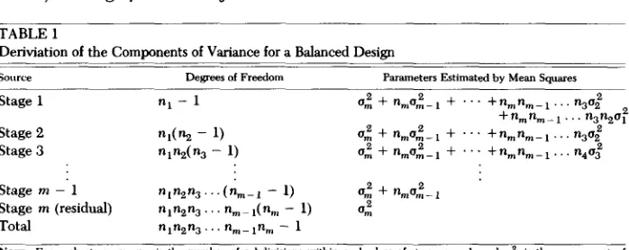
, u:, respectively. They are components of the total variance; thus

TABLE 1

Deriviation of the Components of Variance for a Balanced Design -

Source Degrees of Freedom Parameters Estimated by Mean Squares

Stage 1

Stage 2 Stage 3

Stage rn -'I n , t ~ . p ~ . . . ( n , , - ~ - 1) 0:

+

nma:m2-1 Stage rn (residual) n,n2n3..

.

n,-,(n, - 1)

4

Total n,n2n3. .

.

n,-ln, - 1

NOTE: For each stage ni, nm is the number of subdivisions within each class of stage m - 1, and 0: is the component of variance.

of freedom to obtain the mean squares. It is easy to see then that by starting at the bottom of the table the estimates of the components, u,$ am-,,

. . .

, uI, are computed.

Youden and Mehlich's (1937) inspired contribution was to see that for an attribute distributed in space, the stages could be represented by different distances, and provided these were suitably nested in pairs, the hierarchical model would be valid. They adapted the nested sampling procedure with four stages for soil survey by selecting widely spaced primary stations from which they selected two substations 305 m from one another. Each substation was represented by two further subdivisions 30.5 m apart in each of which were two sampling points

3.05 m apart where the soil was measured. In terms of the analysis in Table 1,

rn = 4, n1 = 9, and n, = n3 = n4 = 2. The components then estimated the con- tributions to the total variance as u: at 3.05 m, u: at 30.5 m, u i at 305 m, and u;

at an average distance somewhat more than 1.6 km.

Finally, the link between the spatial autocorrelation and the results of nested survey was pointed out by Miesch (1975). Where the stages represent distances the accumulated components are semi-variances as defined in equation (7). If we have a nested scheme with rn stages of bifurcation and distances d,, d,,

.

.

.

, d,

between the sampling centers, then

2 2

and so on.

INCREASING ECONOMY

It will be clear from the above that to achieve good spatial resolution over a wide span of ranges demands a large number of stages. Since the sample size at least doubles for each additional stage in a balanced design, nested sampling could readily become prohibitively expensive. Youden and Mehlich's design with only four stages had 9 X 2 x 2

x

2 = 72 sampling points. A fifth and sixth stage would

have required 144 and 288 points, respectively. As it happens, however, full

Stage

1

2

3

4

5

6

7

e

9

Margaret A. Oliver and R. Webster

/

233

7

i

I

Sampling design f o r each centre in example with 5 stages

---

Projected sampling

design for a d d i t i o n a l

stages

FIG. 1. The Unbalanced Hierarchical Sampling Scheme Used in the Nested Survey and a Projected Extension of the Number of Stages to Show the Economy Possible in Such a Design

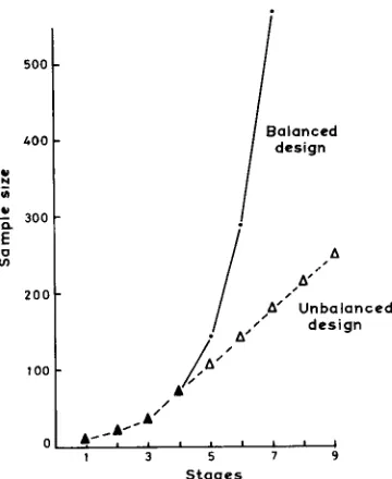
reached. We introduced this innovation in our survey of the Wyre Forest, where with five stages we replicated at only half of the fourth stage units (see below and down to the dashed line in Fig. 1). The main purpose of Figure 1, however, is to show how a hierarchy can be constructed so that at each stage beyond, say, the fourth only half of the sampling centers at the previous stage are replicated. In this way the sampling effort increases only linearly with the number of stages of spatial resolution, rather than geometrically. Figure 2 shows the comparison graphically. There is a small penalty to pay for this lack of balance. The coefficients of the components of variance contributing to the mean squares are no longer simply the sample sizes in each mean. Nor are they the same for a given component in every mean square, and this complicates inferential testing. Gower (1962) and Gates and Shiue (1962) have provided the computational procedure for calculating them, and as it is now in standard texts such as Snedecor and Cocbran (1980), we merely summarize it here. Table 2 shows the coefficients that are required to estimate the components. The computational formula appears complex, but if care is taken to follow the indexing then the procedure is straightforward.

Suppose that there are Ci groups at the ith level and that within the kth group at the ith level there are c , k subgroups at level j , each containing npk, p =

1 , 2 , .

.

.

, c j k , where i

<

j . Then the coefficient uij is given by

Balanced

/

d e s i g n

4c

_ -

I

3 5 7 9

Stages

FIG. 2. Comparison of the Number of Samples Required for Balanced and Unbalanced Nested Sampling Designs

TABLE 2

Denvation of Components of Variance for an Unbalanced Design

~ - _ _

Source Degrees of Freedom Parameters Estimated by Mean Squares

Stage 1 fl

Stage 2

fi

-f, u;_fl;

+

₊

ul,,-p;-l _tl,,,-p;-l

₊

+

_{' . '} ' ' ' _+u,,,u; +u,,,u:

₊

+

_u2,2u; ul,2u;

+

ul,lul"

Stage 3 A - f i u;

+

U3.*-p:-]

+

. ' ' +u3,,u:

Stage m - 1 L,-l - f , - 2 u; + ~ m - l , m - l f l : - l

Stage m N - f m - l

4

Total N - 1

~ ~~~~ -~

N = Sample size

f; = Number of classes at the ith stage.

u , , = j t h coefficient of the variance component at the ith stage.

a,! = Component of variance at the ith stage.

EXAMPLE

Nested Survey

We applied the above principles, including the economy of omitting some of the replication at the lowest level, in a survey of the soil in the Wyre Forest. An earlier survey (Oliver 1984) had suggested that all the spatial variation occurred within distances of 165 m, but because there were few sampling sites closer to one another than this it provided too little information for smaller distances. The semi-variograms of these data show very little change with increasing lag. Figure 3 illustrates this effect for four soil properties: the contents of sand, clay and stones, and mottle percentage at three depths in the profile. There is no spatial autocorrelation at this scale; in geostatistical terms these semi-variograms are pure nugget. The aim of our nested sampling was to confirm this result, and more importantly to discover the structure and measure the scale of the spatial variation at spacings less than

Margaret A. Oliver and R . Webster

/

235

1 0 200 400 wo 800

Mottling

' A A

ALA-

2

L I I 1

0 200 400 600 800

Lag I rn

FIG. 3. Sample and Model Semi-variograms from the First Survey of the Soil of the Wyre Forest, sampled at an average spacing of 167 m, for ( a ) stone content, ( b ) sand content, ( c ) clay content, and ( d ) percentage mottling.

Depths: o 0-5 cm 0 15-20 cm A 40-45 cm

A sampling interval of 6 m was chosen for the lowest stage of the design (Table

3) as we expected this to encompass almost all of the variation. The other intervals were based on a geometrical progression of approximately threefold increments at each stage to incorporate the average spacing of 45 m to 50 m between lithological units, the average sampling interval of the first survey, and a much larger sampling interval in the event of the presence of larger structures. The five-stage sampling design spanned the range from 6 m to 600 m, as described below and illustrated in Figure 4.

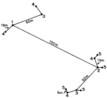
A 600 m grid, with nodes at the grid intersections, was randomly placed over a map of the region to establish the locations of the nine centers for stage 1. From each grid node another point was chosen 190 m away in a random direction to give the second stage. From each of the now 18 points we chose another point 60 m

TABLE 3

Nested Sampling Design for Determining the Scale of Spatial Variation in the Soil of the Wyre Forest

Stage Sampling Interval (meters) Number of Sampling Points 800

190

60 19

6

9 18

36

72

FIG. 4. Spatial Configuration of a Set of Sampling Points from One Center in the Nested Survey

away in a random direction, and repeated the procedure at 19 m to give the fourth stage. From half of the fourth-stage points we chose random points 6 m away (Figs.

1 and 4). A fully balanced survey with 9 first-stage centers would have had

9

x 2 x

2 x 2 x 2 = 144 sampling points. By choosing pairs at only half of the

fourth stage units, however, we contained our sample to 108 (Table 3), resulting in a 25 percent saving of effort. The partitioning of the degrees of freedom and variance was as shown in Table 2. The soil properties were then recorded at four fixed depths in the soil profile: 0 to 5 cm (l), 10 to 15 cm (2), 25 to 30 cm (3), and

50 to 55 cm (4).

Each variate was analyzed following the scheme outlined in Table 2. The estimated components of variance for four of the variates at the four depths are listed in Table 4.

The accumulated components of variance are plotted against distance on a logarithmic scale as semi-variograms (Fig. 5). These graphs and Table 4 indicate that the components of variance for the three lowest stages together account for at least 80 percent of the variation, i.e., a very large proportion of the variation occurs over distances less than 60 m. This pattern of spatial variation is similar for the other properties examined. Stages 1 and 2, i.e., distances between 190 m and

600 m, and 60 m and 190 m, respectively, account for less than 20 percent of the total variation. The estimated component of variance at stage 2 is negative for most of the soil properties. This suggests that variation at this spacing, 190 m, is less than one would expect given the variation at the closer spacings, perhaps because soil features repeat to some extent at that scale. Alternatively, the computed components may estimate zeros in the population, and there is no contribution to the variance at that scale. The confidence limits are wide, and therefore one cannot be sure how to interpret the negative values. There is also considerable residual variation, which represents the variation occurring over distances less than 6 m plus any purely random variation and variation due to measurement error. The spatial variation that remained unresolved at the lowest stage could have been investigated further by adding more stages. This is discussed later.

Transect Sumey

4 -

Y

3 - c

0

.- > k 2 -

1

0

...

:. _.-. -. -. -.

: : ./’ I’

.,ZL

-

”

.

I **

1 1 1 1 ,

400

300

V

0

C

0

0

>

.c 200

100

0

C l a y ...

, I , , (

6 19 60 190 600

....

6001 S a n d ...

400

-

200

-

M o t t l i n g

I 1 1

6 19 60 190 600

S p a c i n g I rn

FIG. 5. Accumulated Components of Variance Plotted against Distance on a Logarithmic Scale for the Soil of the Wyre Forest: ( a ) stone content, ( b ) sand content, ( c ) clay content, and ( d ) percentage mottling.

Depths: 0-5 cm

_____

10-15 cm 25-30 cm . . . 50-55 cm

100 m long and one of 500 m were sampled at 5 m intervals and the same soil properties measured as before. The semi-variances were then estimated by equation

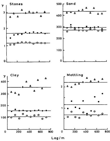
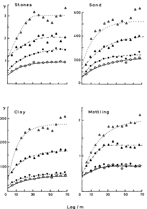
(12) for integer multiples of the sampling interval from 5 m to 70 m. The results for the contents of sand, clay and stones, and for the percentage of mottling are shown in Figure 6.

Following geostatistical practice we have fitted models of smooth curves to the sample estimates. We did this by least squares approximation using Ross’s (1980)

maximum likelihood program. Of the authorized models (Journel and Huijbregts

1978, Oliver and Webster 1986) exponential fimctions provided the best fit, in a least squares sense, for sand, clay and stones, and the spherical model fitted the mottling best. The equations of the models, assuming isotropy, are as follows:

( i ) Exponential:

C,

+

c ( 1 - exp(- h/T)} for h > 0

Margaret A . Oliver and R . Webster

/

239

'1

S t o n e s A A

300 y [ C l a y A A

S a n d

600 r A A

1

M o t t l i n g

A

0 10 30 50 70 0 10 30 50 70

L a g I r n

FIG. 6. Sample and Model Semi-variograms from the Linear Survey of the Soil of the Wyre Forest: ( a ) stone content, ( b ) sand content, ( c ) clay content, and ( d ) percentage mottling.

Depths: 0-0 0-5 cm 0----0 10-15 cm

A- . -A 25-30 cm A . . . . A 50-55 cm

(ii) Spherical:

y ( h ) = c,,

+

c

y ( 0 ) = 0 .

for h > a

In these equations h = lhl, the lag distance, T and a are distance parameters, and

c,, and c are variances.

The parameter a of the spherical model represents a finite limit to the range of spatial dependence, at which the semi-variogram reaches its maximum. Beyond this limit there is no spatial autocorrelation. In these examples the limit occurs at about

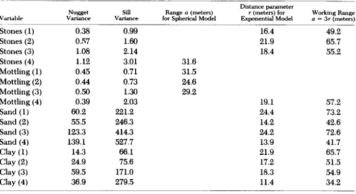
TABLE 5

Parameters of the Models Fitted to the Experimental Semi-variograms of Stone, Sand and Clay Content, and Percentage Mottling at Four Depths in the Soil of the Wyre Forest.

~-

Vanable

Distance parameter

Nugget Sill Range a (meters) r (meters) for Working Range

Variance Variance for Spherical Model Exponential Model a = 3 r (meters)

Stones (1) Stones (2) Stones (3) Stones (4) Mottling (1) Mottling (2) Mottling (3) Mottling (4) Sand (1) Sand (2) Sand (3) Sand (4) Clay (1) Clay (2) Clay (3) Clay (4) 0.38 0.57 1.08 1.12 0.45 0.44 0.50 0.39 60.2 55.5 123.3 139.1 14.3 24.9 59.5 36.9 0.99 1.60 2.14 3.01 0.71 0.73 1.30 2.03 221.2 246.3 414.3 527.7 66.1 75.6 171.0 279.5 16.4 21.9 18.4 31.6 31.5 24.6 29.2 19.1 24.4 14.2 24.2 13.9 21.9 17.2 18.3 11.4 49.2 65.7 55.2 57.2 73.2 42.6 72.6 41.7 65.7 51.5 54.9 34.2

The exponential semi-variograms approach their maxima asymptotically. Nevertheless for practical purposes their ranges are often taken as 3r. An average for the exponential semi-variograms in Table 5 is 55.3 m, which is still within the initially estimated maximum of 60 m.

The quantity c,, known in mining as the nugget variance, is in a sense anomalous. The semi-variance at lag zero is, by definition, itself zero. Yet any reasonable smooth curve fitted through the observed semi-variances in Figure 6 has a positive intercept on the ordinate. The nugget variance appears as the limiting value as h --* 0. In most instances the nugget variance represents spatially dependent variation that occurs over distances smaller than the sampling interval. As Figure 6 and Table 5 show, this variance present within 5 m is still a moderate proportion of the total, c,

+

c.

DISCUSSION AND CONCLUSION

The results from the nested sampling show that almost all of the variance in the

soil properties measured occurs within 60 m. They explain why the semi-variograms

from the earlier survey appeared as pure nugget variance. The interval between neighboring sample points at about 165 m was too large. Only by shortening it could the spatial structure concealed in the nugget variance be exposed. If, as here, nothing is known of that structure then a nested sampling spanning several orders of magnitude in distance should provide a rough semi-variogram of that structure, and in particular indicate its spatial scale.

The results of the transect sampling confirmed this and defined the spatial scale more precisely. They also show the merits of a twephase approach to estimating the semi-variogram as McBratney, Webster, and Burgess (1981) stated.

Margaret A. Oliver and R . Webster

/

241

Using the unbalanced design for nested sampling, the nugget variance can be explored in increasing detail without incurring a huge sampling effort. Stages can be added with only a proportionate rather than geometric increase in effort. In this survey with five stages a 25 percent saving in effort was possible using the unbalanced design, and with more stages the economy would be much greater. If a rough estimate of the scale of spatial variation is all that is required, the nested survey and analysis will suffice.

LITERATURE CITED

Burgess, T. M. and R. Webster (1980). “Optimal Interpolation and Isarithmic Mapping of Soil Properties. I. The Semi-variogram and Punctual Kriging.” J o u m l of Soil Science, 31,315-31.

Burrough, P. A. (1983). “Multiscale Sources of Spatial Variation in Soil. I. The Application of Fractal Concepts to Nested Levels of Soil Variation.” Journal of Soil Science, 34, 577-97.

Campbell, J. B. (1978). “Spatial Variation of Sand Content and pH within Single Continuous Delineations of Two Soil Mapping Units”. Proceedings of the Soil Science Society of America, 42, 460-64.

Cliff, A. D. and J. K. Ord (1981). Spatial Processes: Models and Applications. London: Pion. David, M. (1977). Geostatistical Ore Reserve Estimation. Amsterdam: Elsevier.

Garrett, R. G. (1983). “Sampling Methodology.” In Handbook of Exploration Geochemistry, Vol. 2,

Gates, C. E. and C.

.

Shiue (1962). “The Analysis of Variance of the S-stage Hierarchical Classification.”

Geary, R. C. (1954). “The Contiguity Ratio and Statistical Mapping.” The Zncorporated Statistician, 5,

Gower, J. C. (1962). “Variance Component Estimation for Unbalanced Hierarchical Classification.”

Griffith, D. A. (1979 ‘*Urb% Dominance, Spatial Structure, and Spatial Dynamics: Some Theoretical

Haining, R. P. (1978). “ A Spatial Model for High Plains Agriculture.” Annals of the Association of

Hajrasuliha, S . , N. Baniabbassi, J. Metthey, an!, D. R. Nielsen (1980). “Spatial Variability of Soil

Hammond, L. C., W. L. Pritchett, and U. Chew (1958). “Soil Sampling in Relation to Soil Heterogeneity.”

Jacob, W. C. and A. Klute (1956). “Sampling Soils for Physical and Chemical Properties.” Proceedings

Journel, A. J. and Ch. J. Huijbregts (1978). Mining Geostatistics. London: Academic Press.

Krumbein, W. C. and H. A. Slack (1956). “Statistical Analysis of Low-level Radioactivity of Pennsylvanian Black Fissile Shale in Illinois.” Bulletin of the Geological Society of America, 67, 739-62.

McBratney, A. B. and R. Webster (1986). “Choosing Functions for Semi-variograms of Soil Properties and Fitting Them to Sampling Estimates.” Journal of Soil Science, 37, in press.

A B., R. Webster, and T. M. Burgess (1981). “The Design of Optimal Sampling Schemes

McBratnT

for Loc Estimation .. and Mapping of Regionalized Variables. I. Theory and Method.” Computers and McBratney, A. B., R. Webster, R. G. McLaren, and R. B. Spiers (1982). “Regional Variation of

McCullagh, M. J. (1975). “Estimating by Kriging the Reliability of the Proposed Trent Telemetry

Marcuse, S. (1949). “Optimum Allocation and Variance Components in Nested Sampling with an

Matheron, G. (1965). Les uariables rhgimlishes et leur estimation. Paris: Masson. edited by R. J. Howarth. Amsterdam: Elsevier.

Biometrics, 18, 529-36.

115-45.

Biometrics, 18, 537-42.

and Empirical Impkcations. Economic Geography, 55, 95-113.

American Geographers, 68,493-504.

Sampling for Salinity Studies in Southwest Iran.

Proceedings of the Soil Science Society of America, 22, 548-52.

of the Soil Science Society of America, 20, 170-72.

Irrigation Science, 1, 197-208.

Geosciences, 7, 331-34.

Extractable Copper and Cobalt in the Topsoil of Southeast Scotland.’ Agronomie, 2, 969-82.

Network.” Computer Applications, 2, 357-74.

Application to Chemical Analysis.” B i m t r i c s , 5, 189-206.

(1969). Le krigeage universel. Cahiers du Centre de Morphologie Mathbmatique, No. 1,

Fontainebleau.

Miesch, A. T. (1975). “Variograms and Variance Components in Geochemistry and Ore Evaluation.” In Pantitative Studies in the Geological Sciences, edited by E. H. T. Whitten. Geological Society of America, Memoir 142,333-40.

Moellering, H. and W. Tobler (1972). “Geographical Variances.” Geographical Analysis, 4, 34-50.

Moran, P. A. P. (1948). “The Interpretation of Statistical Maps.” Journal of the Royal Statistical Society, Series B, 10, 243-51.

Nieuwenhuis, J. D. and J. A. Van Den Berg (1971). “Size Investigations in the Morvan.” Reuue de Gomorplwlogie Dynamique, 20, 161-76.

Nortcliff, S. (1978). “Soil Variability and Reconnaissance Soil Mapping: A Statistical Study in Norfolk.” Journal of Soil Science, 29, 403-18.

Oliver, M. A. (1984). Soil Variation in the Wyre Forest: Its Elucidation and Measurement. Ph.D. dissertation, University of Birmingham.

Oliver, M. A. and R. Webster (1986). “Semi-variograms for Modelling the Spatial Pattern of Landform and Soil Properties.” Earth Surface Processes and Landforms, 11, in press.

Olson, J. S. and P. E. Potter (1954). “Variance Components of Cross-bedding Direction in Some Basal Pennsylvanian Sandstones of the Eastern Interior Basin: Statistical Methods.” Journal of Geology, 62, 26-49.

Ross, G. J. S. (1980). MLP Maximum Likelihood Program. Rothamsted Experimental Station, Harpenden. Russo, D. (1984). “Statistical Analysis of Crop Yield-Soil Water Relationships in Heterogeneous Soil

under Trickle Irrigation.” Soil Science Society of America Journal, 48, 1402-10.

Snedecor, G. W. and W. G . Cochran (1980). Statistical Methods. 7th ed. Ames: Iowa State University Press.

Thornes, J. B. (1973). “Markov Chains and Slope Series: The Scale Problem.” Geographical Analysis, 5, 322-28.

Tidball, R. R. and R. C. Severson (1976). “Chemistry of Northern Great Plains Soils.” United States Geological Suruey, Open File Report, 76729, 57-81.

Verly, G., M. David, A. G. Joumel, and A. Marechal, eds. (1984). Geostatistics for Natural Resources Characterization, Parts 1 and 2. Dordrecht: Reidel.

Webster, R. (1985). “Quantitative Spatial Analysis of Soil in the Field.” Aduances in Soil Science, 3, 1-70.

Webster, R. and B. E. Butler (1976). “Soil Classification and Survey Studies at Ginninderra.” Australian Journal of Soil Research, 14, 1-24.

Webster, R. and M. A. Oliver (1985). “Utilisation exploratoire de la gkostatistique pour la cartographie du sol dans la forGt de Wyre (G.B.).” Sciences de la Terre, SMe Z n f m t i q u e Gologique, 24, 162-73.