University of New Orleans University of New Orleans
ScholarWorks@UNO
ScholarWorks@UNO
University of New Orleans Theses and
Dissertations Dissertations and Theses
Summer 8-6-2018
Generalizing Multistage Partition Procedures for Two-parameter
Generalizing Multistage Partition Procedures for Two-parameter
Exponential Populations
Exponential Populations
Rui Wang
University of New Orleans, [email protected]
Follow this and additional works at: https://scholarworks.uno.edu/td
Part of the Applied Statistics Commons, Probability Commons, Statistical Methodology Commons, and the Statistical Models Commons
Recommended Citation Recommended Citation
Wang, Rui, "Generalizing Multistage Partition Procedures for Two-parameter Exponential Populations" (2018). University of New Orleans Theses and Dissertations. 2510.
https://scholarworks.uno.edu/td/2510
This Dissertation-Restricted is protected by copyright and/or related rights. It has been brought to you by ScholarWorks@UNO with permission from the rights-holder(s). You are free to use this Dissertation-Restricted in any way that is permitted by the copyright and related rights legislation that applies to your use. For other uses you need to obtain permission from the rights-holder(s) directly, unless additional rights are indicated by a Creative Commons license in the record and/or on the work itself.
This Dissertation-Restricted has been accepted for inclusion in University of New Orleans Theses and Dissertations by an authorized administrator of ScholarWorks@UNO. For more information, please contact
Generalizing Multistage Partition Procedures for Two-parameter
Exponential Populations
A Dissertation
Submitted to the Graduate Faculty of the University of New Orleans
in partial fulfillment of the requirements for the degree of
Doctor of Philosophy
in
Engineering and Applied Science Mathematics
by
Rui Wang
M.S. University of New Orleans, 2014
B.S. Huazhong University of Science and Technology, 2010
Acknowledgments
I would like to give my sincere gratitude toward Professor Tumulesh Solanky, who
gener-ously spent considerable time in the past few years on discussing lots of details presented
in this dissertation. Professor Solanky also read through the earlier draft of this
disser-tation with great patience and presented many valuable suggestions, without which, I
believe, there is still a long way for it to take the present form. I would like to thank
other four committee members,
Professor Linxiong Li Department of Mathematics,
Professor Jairo Santanilla Department of Mathematics,
Professor Vesselin P Jilkov Department of Electrical Engineering,
Professor Huimin Chen Department of Electrical Engineering,
for their advice and suggestions where contributed in several aspects to this dissertation.
Contents
List of Tables vi
Abstract viii
1 Introduction 1
1.1 Introduction of Exponential Distribution . . . 1
1.2 Parameter Estimation . . . 5
1.3 Bayesian Inference . . . 7
1.4 Two-parameter Exponential Distribution . . . 8
1.5 Ranking and Partition Problems . . . 11
1.6 Formulation . . . 12
1.6.1 Indifference Zone Approach . . . 13
1.6.2 Random Subset Approach . . . 13
1.7 Selecting Best Normal Populations . . . 15
1.8 Selecting Best Two-parameter Exponential Populations . . . 17
1.9 Partition Problem . . . 20
2 Partition Problem for Exponential Distributions 24 2.1 Formulation for Partitioning Two-parameter Exponential Distributions . . 25
2.3 LFC Validation . . . 38
2.4 Single-stage Procedure . . . 44
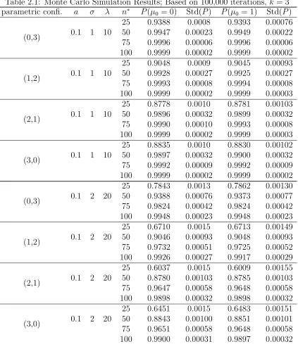
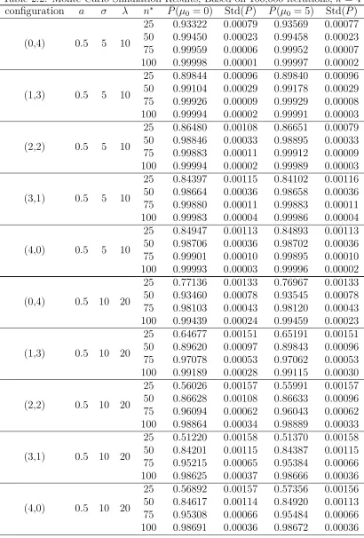
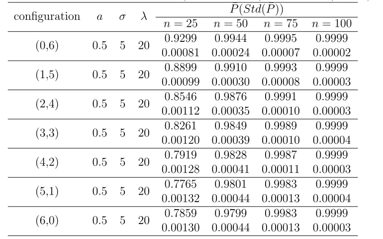
2.5 Monte Carlo Simulation Study of Single-stage Procedure . . . 53
3 Multistage Methodology for the partition problem 58 3.1 Purely Sequential Selection . . . 58
3.2 Asymptotic Properties of Purely Sequential Procedure . . . 60
3.3 Monte Carlo Simulation Study of Purely Sequential Procedure . . . 66
4 Two-stage Selection Procedure 70 4.1 Two-stage Selection . . . 70
4.2 Asymptotic Properties of Two-stage Procedure . . . 71
4.3 Monte Carlo Simulation Study of Two-stage Procedure . . . 79
4.4 Concluding Remarks and Future Work . . . 79
Bibliography 82
List of Tables
2.1 Monte Carlo Simulation Results; Based on 100,000 iterations, k= 3 . . . . 40
2.2 Monte Carlo Simulation Results; Based on 100,000 iterations, k= 4 . . . . 41
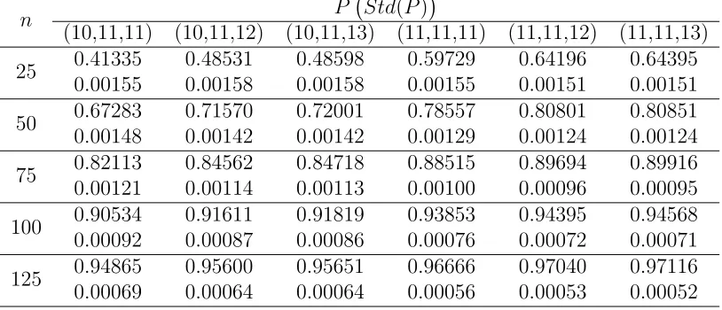
2.3 Monte Carlo Simulation Results of (µ1, µ2, µ3); Based on 100,000 iterations,
indifference zone=(10,11), σ = 20, k= 3 . . . 42
2.4 Monte Carlo Simulation Results of (µ1, µ2, µ3, µ4); Based on 100,000
itera-tions, indifference zone=(10,11), σ = 20,k = 4 . . . 42
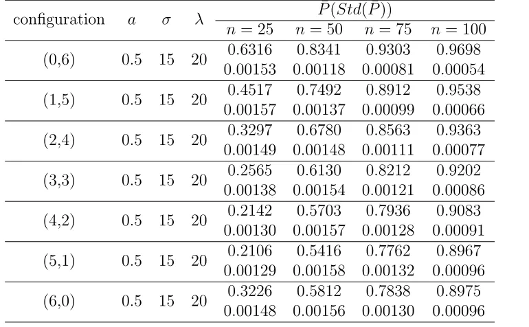
2.5 Monte Carlo Simulation Results; Based on 100,000 iterations, σ= 5, k = 6 43
2.6 Monte Carlo Simulation Results; Based on 100,000 iterations, σ= 10, k = 6 43
2.7 Monte Carlo Simulation Results; Based on 100,000 iterations, σ= 15, k = 6 44
2.8 Value of constantb satisfying (2.14) . . . 47
2.9 Simulation of Single-stage Procedure (2.4.1); Based on 100,000 iterations,
P∗ = 0.9 and n∗ =50, k=4 . . . 56
2.10 Simulation of Single-stage Procedure (2.4.1); Based on 100,000 iterations,
P∗ = 0.95 andn∗ =50, k=4 . . . 56
2.11 Simulation of Single-stage Procedure (2.4.1); Based on 100,000 iterations,
P∗ = 0.9 and n∗ =50, k=6 . . . 57
2.12 Simulation of Single-stage Procedure (2.4.1); Based on 100,000 iterations,
P∗ = 0.95 andn∗ =50, k=6 . . . 57
3.2 Simulation of The purely Sequential Procedure (3.3); Based on 100,000
iterations, p∗ =0.9,k=4, m =5 . . . 68
3.3 Simulation of The purely Sequential Procedure (3.3); Based on 100,000 iterations, p∗ =0.95,k=4, m =5 . . . 68
3.4 Simulation of The purely Sequential Procedure (3.3); Based on 100,000 iterations, p∗ =0.99,k=4, m =5 . . . 69
4.1 Critical Constant value ofh, as defined in (4.4) for P∗ = 0.9 . . . 76
4.2 Critical Constant value ofh, as defined in (4.4) for P∗ = 0.95 . . . 77
4.3 Critical Constant value ofh, as defined in (4.4) for P∗ = 0.99 . . . 78
4.4 Simulation of Two-stage Procedure (4.1); Based on 100,000 iterations, p∗ =0.95,k=4, m =5 . . . 79
4.5 Simulation of Two-stage Procedure (4.1); Based on 100,000 iterations, p∗ =0.9, k=4, m =5 . . . 80
4.6 Simulation of Two-stage Procedure (4.1); Based on 100,000 iterations, p∗ =0.99,k=4, m =5 . . . 80
4.7 Simulation of Two-stage Procedure (4.1); Based on 100,000 iterations, p∗ =0.9, k=4, m =10 . . . 80
Abstract
ANOVA analysis is a classic tool for multiple comparisons and has been widely used in
numerous disciplines due to its simplicity and convenience. The ANOVA procedure is
designed to test if a number of different populations are all different. This is followed by usual multiple comparison tests to rank the populations. However, the probability of
selecting the best population via ANOVA procedure does not guarantee the probability
to be larger than some desired prespecified level. This lack of desirability of the ANOVA
procedure was overcome by researchers in early 1950’s by designing experiments with the
goal of selecting the best population. In this dissertation, a single-stage procedure is
in-troduced to partition k treatments into “good” and “bad” groups with respect to a control
population assuming some key parameters are known. Next, the proposed partition
proce-dure is genaralized for the case when the parameters are unknown and a purely-sequential
procedure and a two-stage procedure are derived. Theoretical asymptotic properties, such
as first order and second order properties, of the proposed procedures are derived to
doc-ument the efficiency of the proposed procedures. These theoretical properties are studied
via Monte Carlo simulations to document the performance of the procedures for small
and moderate sample sizes.
Key words: Two-parameter Exponential Distribution; Sequential Procedure;
Probability of Correct Decision; Indifference Zone;
1
Introduction
1.1 Introduction of Exponential Distribution
How long will a piece of machinery work without breaking down? How much time will
elapse before an earthquake occurs in a given region? How long do we need to wait before
a customer enters a shop? How long will it take before a call center receives the next
phone call? All these questions above concern the time we need to wait before a given
event occurs. If this waiting time is unknown, it is often appropriate to think it of as
a random variable having an exponential distribution. The time we need to wait before
a certain event occurs follows exponential distribution if the probability that the event
occurs during a certain time interval is proportional of the length of that time interval.
The probability density function (PDF) of an exponential distribution is
f(x;λ) =
λe−λx x≥0,
0 x <0.
(1.1)
The parameter λ is called rate parameter. It is the inverse of the expected duration
cumulative distribution function (CDF) of an exponential distribution is given as
F(x;λ) =
1−λe−λx x≥0
0 x <0.
(1.2)
Alternatively, this can be defined using the Heaviside step function H(x) as
F(x;λ) = (1−e−λx)H(x). (1.3)
The cumulative density function (CDF) can be written as the probability of the lifetime
being less than some value x, which is given as
P(X ≤x) = 1−e−λx. (1.4)
A commonly used alternative parametrization is to define the probability density
func-tion (pdf) of an exponential distribufunc-tion as
f(x;β) =
1
βe −x
β x≥0,
0 x <0.
(1.5)
whereβ >0 is mean, standard deviation, and is also known as the scale parameter of the
distribution, the reciprocal of the rate parameter, λ, defined above. In this specification,
β is a survival parameter in the sense that if a random variable X is the duration of time
that a given biological or mechanical system manages to survive and X ∼ Exp(β) then
E[X] = β. That is to say, the expected duration of survival of the system is β units of
time. The parametrization involving the ”rate” parameter arises in the context of events
arriving at a rate λ, when the time between events (which might be modeled using an
The alternative specification is sometimes more convenient than the one given above,
and some authors will use it as a standard definition. This alternative specification is not
used in this chapter.
The expected value of an exponential variable X is :
E[X] = 1 λ.
The variance of an exponential variable X is :
V ar[X] = 1 λ2,
so one properties of the exponential distribution is that the standard deviation and the
mean of the distribution are equal. The moments of X, for n = 1, 2, ..., are given by
E[Xn] = n! λn.
The median of X is given by
m[X] = ln(2)
λ < E[X],
where lnrefers to the natural logarithm. Thus the absolute difference between the mean
and median is
|E[X]−m[X]|= 1−ln(2) λ <
1
λ = standard deviation,
An exponentially distributed random variable T obeys the relation
P(T > s+t|T > s) = P(T > t), ∀s, t≥0.
When T is interpreted as the waiting time for an event to occur relative to some initial
time, this relation implies that, if T is conditioned on a failure to observe the event over
some initial period of time s, the distribution of the remaining waiting time is the same as
the original unconditional distribution. For example, if an machine has not broken after
10 years, the conditional probability that fail will take place after at least 10 more years
is equal to the unconditional probability of observing the fail after more than 10 years
relative to the initial time.
The exponential distribution and the geometric distribution are the only memoryless
probability distributions. The exponential distribution is consequently also necessarily
the only continuous probability distribution that has a constant failure rate. That’s why
the exponential distribution the very commonly used in reliability engineering.
The mathematics associated with the exponential distribution is often of a simple
na-ture, and so it is possible to obtain explicit formulas in terms of elementary functions,
without to obtain troublesome quadrature. For this reason models constructed from
ex-ponential variables are sometimes used as an approximate representation of other models
that are more appropriate for a particular application. Currently among the most
promi-nent applications are in the field of life-testing. The lifetime(or life characteristic, as it is
often called) can be usefully represented by an exponential random variable, with a
rel-atively simple associated theory. Sometimes the representation is not adequate; in such
cases a modification of the exponential distribution (often a Weibull distribution) is used.
Another application is producing usable approximate solutions to difficult
a sequential procedure is due to Ray (1957). He wished to calculate the distribution of
the smallest n for which Pn
i=1Ui2 < Kn, where U1, U2, . . . are independent unit normal
variables and K1, K2, . . . are specified positive constants. By replacing this by the
dis-tribution of the smallest even n, he obtained a problem in which the sums Pn
i=1U 2
i are
replaced by sums of independent exponential variables(actually χ2,s with two degrees of
freedom each).
1.2 Parameter Estimation
Before 1959 a considerable amount of work had been done on inference procedures for
the exponential distribution with both censored and uncensored data. It was realized, in
the 1960s and 1970s, that although the exponential distribution can be handled rather
easily, the consequent analysis is often poorly robust [see Zelen and Dannemiller (1961)].
Nevertheless, the study of properties of this distribution, and especially construction of
estimation and testing procedures has continued steadily, during the last 30 years, with
some emphasis on Bayesian analysis and order statistics methodology, and an explosion
and results on characterizations.
Maximum likelihood estimation is one of the most useful technique which derives
estimates of the unknown parameters by maximizing a likelihood function constructed
through the available data. Suppose, a given variable X is exponentially distributed and
the rate parameter λ is to be estimated. Then, the likelihood function, given by an
independent and identically distributed sample X = (x1,· · · , xn), is given by
L(λ) = Qn
i=1λe
−xiλ =λne−λPni=1xi
=λne−λn¯x,
where ¯x= n1 Pn
The first derivative of the likelihood function’s logarithm is:
d
dλln(L(λ)) = d
dλ(nln(λ)−λnx¯)
= nλ −nx¯
>0 if 0< λ < 1x¯, = 0 if λ= ¯x,
<0 if λ > x1¯.
The second derivative is easily obtained as
d2
dλ2ln(L(λ)) = −
1 λ2 <0.
Consequently the maximum likelihood estimate for the rate parameter is
ˆ λ= 1
¯ x.
Another classic method of parameter estimation is Moment generation method, which
uses the moments of the distribution to estimate the parameter. Since the density function
of exponential distribution only contains one single parameter λ, only first moment is
needed.
E[x] =
Z ∞
0
xf(x)dx=
Z ∞
0
xλe−λxdx
=−
Z ∞
0
xde−λx
= [−xe−λx]∞0 +
Z ∞
0
e−λxdx
=h− 1 λe
−λxi∞
0 = 0 +
1 λ =
1 λ.
Then let E[x] = ¯x, we have
So the moment generating estimator for the rate parameter is
˜ x= 1
¯ x.
1.3 Bayesian Inference
In Bayesian probability theory, if the posterior distribution p(θ|x) and the prior
prob-ability distribution p(θ) are in the same family, then the posterior and prior are called
conjugate distribution, and the prior is called a conjugate prior for the likelihood
func-tion. For instance, the Gaussian family is self-conjugate to Gaussian likelihood function
if the likelihood function is Gaussian. In order to have the posterior distribution to be
Gaussian, one needs to choose a Gaussian prior over the mean. This means that Gaussian
distribution is a conjugate prior for its likelihood function which is also Gaussian.
Sim-ilarly, the conjugate prior for the exponential distribution is the gamma distribution(of
which the exponential distribution is a special case). The following parametrization of
the gamma probability density function is useful:
Gamma(λ;α, β) = β
α
Γ(α)λ
α−1
exp(−λβ). (1.6)
The posterior distribution p can then be expressed in terms of the likelihood function
defined above and a gamma prior:
p(λ)∝L(λ)×Gamma(λ;α, β)
=λnexp (−λnx)× β α
Γ(α)λ
α−1exp(−λβ)
∝λ(α+n)−1exp(−λ(β+nx)).
Since it has the form of a gamma pdf, this can easily be filled in, and one obtains:
p(λ) = Gamma(λ;α+n, β+nx).
Here the hyperparameter α can be interpreted as the number of prior observations,
and as the sum of the prior observations. The posterior mean here is:
α+n β+nx.
1.4 Two-parameter Exponential Distribution
One commonly used generalization of the exponential distribution is the two-parameter
exponential distribution. The density function is given as:
fX(x) =σ−1exp{−(x−θ)/σ}I(x > θ), (1.7)
where σ is the scale parameter, which is equal to λ1 shown in preview sections. And θ is the location parameter.For variables following two-parameter exponential density
function, the possible values varies from θ to∞. θ can be considered equal to 0 respect
to one-parameter exponential distribution.
Similar to the properties with classic one-parameter exponential distributions, some
useful results are shown as below; The expected value of a two-parameter exponential
variable X is :
E[X] =θ+σ.
The variance of an exponential variable X is :
So the standard deviation of the distribution is equal toσ. And the maximum likelihood
estimator and moment generating estimator of σ is 1nPn
i=1(xi − θ). If X1, X2, . . . , Xn
are independent random variables each following two-parameter exponential distribution,
then the maximum likelihood estimators of θ and σ are
ˆ
θ =min(X1, X2, . . . , Xn),
ˆ σ = 1
n n
X
i=1
(Xi−θˆ) = ¯X−θ.ˆ
Ifθ is known, the maximum likelihood estimator of σ is ( ¯X−θ). Even with σ known,
ˆ
θ above is still the maximum likelihood estimator ofθ. The probability density function
of ˆθ is
fθˆ(x) = (n/θ)exp{−n(x−θ)/σ}I(x > θ),
which is of the same form as (1.7) but with σ replaced by σ/n. The variance of ˆθ is
therefore σ2/n2, and its expected value is θ +σ/n. It is interesting to note that the
variance is proportional to n−2 and not to n−1. The expected value of ˆσ[= ¯X −θˆ] is
σ(1−n−1), and its variance isσ2[n−1+n−2−2n−3]. And the expected value of ( ¯X−θ)
is σ and its variance is σ2n−1.
Moment estimators (˜θ,σ˜) of (θ, σ) can be obtained by equating sample and population
values of the mean and variance. They are
˜
θ = ¯X−σ,˜
˜ σ2 = 1
n n
X
i=1
Xi2.
Cohen and Helm (1973) discuss modified moment estimators obtained by replacing
its expected value. This gives
˜
θ∗ +n−1σ˜∗ =X0
1,
which leads to
˜
θ∗ = nX 0
1−X¯
n−1 ,
˜
σ∗ = n( ¯X−X 0
1)
n−1 .
They show that these are minimum variance unbiased estimators (and a fortiori BLUEs).
Also
V ar( ˜θ∗) = σ
2
n(n−1), (1.8)
V ar( ˜σ∗) = σ
2
n−1, (1.9)
Cov( ˜θ∗,σ˜∗) = σ
2
n(n−1), (1.10)
so that Corr( ˜θ∗,σ˜∗) = 1/√n. Further, since ˜σ∗ is distributed as 1
2(n −1)
−1χ2
2(n−1), a
100(1−α)% confidence interval for σ is
2(n−1)
χ2
2(n−1),1−α
2
˜
σ∗, 2(n−1) χ2
2(n−1),α2
˜
σ∗. (1.11)
Two-parameter exponential distribution has been used extensively in many reliability
and life testing experiments for describing the failure rates of complex equipment, vacuum
tubes and so on. It has also been recommended as a statistical model in clinical trials,
such as the studies of behavior of tumor systems in animals and analysis of survival data
in cancel research. The relative applications can be found in Johnson and Kotz (1994),
1.5 Ranking and Partition Problems
In everyday life, one decides on the best medicine, best machine, best strategy or the
best route for a destination, among a number of available options. In the statistical
literature, such selections have been routinely carried out under the area of multiple
comparisons. A commonly used statistical tool called Analysis of Variance (ANOVA)
has been used extensively by practitioners to test whether or not the given treatments
under consideration are all same or not. Generally, the ANOVA test is followed by some
multiple comparisons tests, such as, LSD, Tukey Method, Scheffe Method to name a
few, to decide which treatments are different from one another. However, those methods
perform shortage in reality when implementation.
For example in clinical trials, a usual concern is comparing efficacy of the several
essentially different varieties of drugs. A conclusion that whether those different drugs
have the same efficacy or not can be easily obtained by setting that as the null hypotheses
using above methods, which is meaningless. One main reason is that those different
varieties of drugs tend to perform differently in most cases. But that is far away from
enough to make any market value. Because rather than detecting the difference of the
efficacy among those varieties of drugs, the experimenters are more willing to explore the
one or several drugs that show better efficacy. So detecting the best or worst drugs is the
need, which helps with business strategy making, which ANOVA and those comparison
tests can not help achieve.
Thus, the experimenter’s problem should not be only testing the equality of efficacy of
these drugs, but rather to select the best one. The definition of the best would vary from
situation to situation and it is generally for the experts in the area to dictate what best
means in a given situation. For example, in some clinical trials. Sometimes, practitioners
the ranking of the means without realizing that the ANOVA test is designed to test if the
given treatments are all same or not. The ANOVA test is not designed to select the best
treatment and one cannot associate a probability statement with the selected treatment
as being the best via the ANOVA approach.
In a pioneer work, Bechhofer (1954) introduced the concept of indifference-zone
formu-lation and formulated some methodologies for the problem of selecting the best treatment
from a set of several treatments. The formulation by Bechhofer had the desired property
of selecting the best treatment with the pre-specified probability of correct selection. The
formulation proposed by Bechhofer (1954) is referred to as the indifference-zone
formu-lation in the statistical literature. Around the same time, Gupta (1956) formulated a
strategy which controls the probability of correct selection in the whole parameter space,
as opposed to the preferencezone which was the case under Bechhofers approach. The
formulation of Gupta (1956), selects a subset of random size which includes the best
treat-ment with some pre-specified probability. The formulation proposed by Gupta (1956) is
referred to as the subset-selection formulation in the statistical literature.
1.6 Formulation
In this section, the idea of two most fundamental approaches in the area of selection and
ranking are introduced under a classic case of population partition problem. Suppose
we have πi, i = 1, . . . , k(≥ 2), independent normally distributed populations, having
unknown means µi and common unknown variance σ2. We assume that µi ∈ R and σ ∈ R+, i =1,...k. Let µ[1], . . . , µ[k] be the ordered µ-values, Since the variance is same
among all populations, we sample equally from each population and at any point of time,
whenever we need new” samples from π,s, we take a certain equal number, to be made
associated with µ[k], and such a population is called the best population. We assume
that there is just one population associated with µ[k]. We do not, however assume any
knowledge about the association of the µ,is with µ,[i]s.
1.6.1
Indifference Zone Approach
Next, Bechhofer’s (1954)indifference zone approach is introduced. Givenδ∗ >0, we define
Ω ={µ= (µ1, ..., µk) :µi ∈R, i= 1, ..., k},
Ω(δ∗) ={µ= (µ1, ..., µk) :µ[k]−µ[k−1] ≥δ∗},
where Ω is the whole parameter space forµand Ω(δ∗) is called the preference zone. For a
given P∗ ∈(k−1,1), we are interested in selection procedures such that the probability of
correct selection (CS) of the population associated withµ[k]is at leastP∗or asymptotically
(as δ∗ → 0) at least P∗ whenever the true parameter µ ∈ Ω(δ∗). In other words, we
are interested to identify the best population having certain minimum or approximately
minimum probabilityP∗ that our final decision is the right one when the best population’s
mean is at least δ∗-unit ahead of the mean of the second best. The parameter space
Ω(δ∗) is called, the preference zone, while ΩC(δ∗)(= Ω−Ω(δ∗)) is called the indifference
zone in the sense that the experimenter is not willing to pick the best population when
µ[k]−µ[k−1] < δ∗, that is the experimenter expresses indifference in the parameter space
ΩC(δ∗). Because for the indifference zone ΩC(δ∗) the best population is apparently not
that much better than the second best.
1.6.2
Random Subset Approach
Gupta (1956) assigned a procedure for selecting a subset such that the probability that
greater than a predetermined number P∗. His goal is to separate those treatments which
are better than the control from those that are worse(or not better). Considering the
problem of selecting the best one of k categories when comparing k-1 categories with a
control or standard, he controls the probability of selecting the standard as the best when
the categories are equal to(or worse than) the control. Retain in the selected subset those
and only those populations Ω[i](i= 1,2, ..., k) for which
¯
x[i]≥µ0−dσ/
√ ni.
To determine the value of d letk1,k2 denote the true number of populations with µ≥µ0
and µ < µ0, respectively, so that k1+k2 =k. The the probability P of retaining all the
k1 populations with µ≥µ0 is given by
P =
k1
Y
i=1
P{x¯0i ≥µ0−dσ
p
n0 i}
=
k1
Y
i=1
P{pn0 i(¯x
0−µ0
i)/σ ≥ −d+
p
n0
i(µ0−µ0i/σ}. (1.12)
where primes refer to values associated with the k1 populations for which µ≥µ0. Hence
P =
k1
Y
i=1
{1−F(−d+pni0(µ0−µ0i)/σ},
where F(x) refers to the standard normal cumulative distribution function. Theµ0i above
are restricted by the condition µ0i ≥ µ0 and minimum of equation above is attained by
setting µ0i =µ0(i= 1,2, ..., k1). Now since result depends on the unknown integer k1, we
can obtain a lower bound by settingk1 =k. Then using the symmetry of F we have
The equation determining d is obtained by setting the right-hand member of equation
above equal to P∗ and is given by
F(d) = (P∗)1/p.
1.7 Selecting Best Normal Populations
As mentioned in preview sections, under some cases checking whether the means of several
populations are equal or not is far from enough. People need to find the ”best” one which
have the greatest location parameter. In this section we derive this problem under the
setting of Indifference-Zone from Bechhofer. Mukhopadhyay, N. and Solanky, T.K.S.
(1994) also summarize the relative results.
Suppose that we have k(≥) independent, normally distributed populationsπ1, . . . , πk,
with unknown mean µi and common unknown variance σ2, with the density function
given by
f(xij) = 1/ √
2πσ2exp{−(x
ij −µi)2/2σ2}. (1.13)
Let us define the following:
¯
Xi =n−1
Pn
j=1Xij,
Vi = (n−1)−1Pnj=1(Xij −X¯i)2,
ˆ
σ2 =Pk
i=0
Pn
j=1(Xij −X¯i)
2/((k+ 1)(n−1)),
(1.14)
where ¯Xi is the point estimate of µi and ˆσ is the pooled estimate of σ if a common
unknown standard deviation is assumed. And µ[1], . . . , µ[k] are defined as the ordered
µ-values. Right now it is assumed that σ is known and Xi1, . . . , Xin from πi have been
recorded. The natural selection rule is simply to pick the population associated with the
R∗: Selectπj as the best population if ¯Xjn=M ax1≤i≤kX¯in.
It is denoted that φ(y) = (2π)−12exp(−y2/2) and Φ(y) = Ry
−∞φ(x)dx, for all y ∈ R.
Let π(i) stand for the population associated with the location parameter µ[i] and let us
write ¯X(in) for the sample mean arising from the population π(i), i= 1, . . . , k. Also, write
δi = µ[k]−µ[i] and note that δi ≥ 0 for arbitrary µ ∈ Ω(δ∗)∪Ωc(δ∗) and δi ≥ δ∗ for
arbitrary µ∈Ω(δ∗). Then, the probability of correct selection is given by
Pn(CS) =P{X¯kn >X¯in, i= 1, . . . , k−1}
=P{n12σ−1( ¯Xkn−µ[k]) +n 1
2σ−1(µ[k]−µ[i])> n 1
2σ−1( ¯Xin−µ[i]), i= 1, . . . , k−1}
=P{Ykn+n 1
2δiσ−1 > Yin, i= 1, ..., k−1},
whereYin =n 1
2( ¯Xin−µ[i])/σ, i= 1, ..., k, which is following a standard normal distribution.
From equation above, for all µ∈Ω(δ∗),
Pn(CS) =
R∞
−∞
Qk−1
i=1 Φ(y+n
1
2δiσ−1)φ(y)dy ≥R∞
−∞Φ(y+n 1
2δ∗σ−1)φ(y)dy,
where the equality holds whenδi =δ∗for alli= 1, ..., k−1. Thereforeµ[1] =· · ·=µ[k−1] =
µ[k]−δ∗, a parameter configuration is referred to as the least favorable configuration(LFC).
Hence,
Infµ∈Ω(δ∗)Pn(CS) =
Z ∞
−∞
Φ(y+n12δ∗σ−1)φ(y)dy, (1.15)
while this infimum is attained at the LFC. Let h=h(k, P∗) be such that
Z ∞
−∞
[Φ(y+h)]k−1φ(y)dy=P∗, (1.16)
then it follows that Pn(CS) ≥ P∗ for all µ ∈ Ω(δ∗) when n ≥ h2σ2/δ∗2 = C. In other
implement the corresponding selection rule above to pick the best normal distribution in
order to meet theP∗ requirement for P(CS) in Ω(δ∗). HoweverC is unknown. Moreover,
one can show that there exists no fixed-sample size procedure that will meet the P∗
requirement for P(CS) in Ω(δ∗), uniformly in σ ∈ R+. The values of ”h” was tabulated in Bechhofer (1954). For the case of σ being unknown, a two-stage procedure had been
proposed by Bechhofer et al. (1954) and a purely sequential procedure had been proposed
by Robbins et al. (1968).
1.8 Selecting Best Two-parameter Exponential
Populations
Two-parameter exponential model has applications in many fields. In reliability and
en-gineering, the location parameter is guarantee life of a component and scale parameter
is the average life. When distribution is used to model the life lengths in dose-response
experiments, location and scale parameters are referred as guaranteed and average
effec-tive duration of a drug respeceffec-tively. For some applications of two-parameter exponential
model one may refer to Johnson and Kotz (1994), Bain and Engelhardt (1991), Lawless
and Singhal (1980), Zelen (1966).
Many researchers have discussed the problem of simultaneous comparisons of
exponen-tial location parameters when scale parameters are equal or unequal under
heteroscedas-ticity. Ng et.al (1993) proposed multiple comparison procedures with control when scale
parameters are equal. Wu et al. (2010) developed one-stage procedure of multiple
com-parisons with the control for exponential location parameters under heteroscedasticity.
The procedures proposed by these researchers make use of Lam (1987,1988) technique to
construct SCIs(Simultaneous Confidence Intervals).
their location parameters come from the setting of Indifference-Zone as mentioned in
previews sections which originated in comparing several normal populations.
Suppose that we have k(≥ 2) independent and exponentially population π1, ..., πk,
with density function of πi :i= 1,2, . . . , k given by
fX(x) = σ−1exp{−(xij −θi)/σ}I(xij > θi). (1.17)
Let us define the following:
Ti =M in1≤j≤n{Xi1, ..., Xin}, Vi = (n−1)−1Pjn=1(Xij −Ti),
ˆ
σ =Pk
i=0
Pn
j=1(Xij −Ti)/((k+ 1)(n−1)),
(1.18)
whereTi are the order statistic or point estimate ofθi and ˆσ is the pooled estimate ofσ if
a common unknown scale parameter is assumed. The density function of T is derived as
F(T) =P(T ≤t) = 1−P(T > t) = 1−P(X1 > t, X2 > t, . . . , X(n)> t)
= 1−Qn
i P(Xi > t) = 1−
Qn
i[1−F(Xi)]
= 1−[1−F(t)]n.
Since F(X) = 1−e−x−σθ, X > θ, then the cumulative function and density function of T
are obtained as
FT(t) = 1−e−
n(t−θ)
σ t > θ,
fT(t) = [F(T)]
0
= nσe−n(tσ−θ) t > θ.
(1.19)
It is clear thatTis are following exponential distribution with location parameter ofθ and
scale parameter of σn. Here θ[1], . . . , θ[k] are defined as the ordered θ-values. The partition
distribution, which has the largest or smallest location parameter. It is assumed that σ
is known and the observations Xi1, ..., Xin from πi, i= 1, . . . , k have been recorded. The
natural selection rule is simply to pick the population associated with the largestTi value,
i = 1,..., k, which is procedure
R∗: Selectπj as the best population if Tj =M ax1≤i≤kTin.
Let π(i) stand for the population associated with the location parameter θ[i] and let
us write Tin for the sample minimum arising from the population π(i), i = 1, ..., k. Also,
write δi =θ[k]−θ[i] and note that δi ≥0 for arbitrary θ ∈Ω(δ∗)∪Ωc(δ∗) and δi ≥δ∗ for
arbitrary θ∈Ω(δ∗). Then, the probability of correct selection is given by
Pn(CS) =P{Tkn > Tin, i= 1, ..., k−1}
=P{nσ−1(Tkn−θ[k]) +nσ−1(θ[k]−θ[i])> nσ−1(Tin−θ[i]), i= 1, ..., k−1}
=P{Zkn+nδiσ−1 > Zin, i= 1, ..., k−1},
where Zin = n{Tin − θ[i]}/σ, i = 1, ..., k, which are all following standard exponential
distribution. From equation above, for all θ ∈Ω(δ∗),
Pn(CS) =
R∞
0
Qk−1
i=1[1−exp(−z−nδiσ
−1)]exp(−z)dz
≥R∞
0 [1−exp(−z−nδ
∗σ−1)]k−1exp(−z)dz,
where the equality holds whenδi =δ∗for alli= 1, ..., k−1. Thereforeθ[1] =· · ·=θ[k−1] =
θ[k]−δ∗, a parameter configuration is referred to as the least favorable configuration(LFC).
Hence,
Infθ∈Ω(δ∗)Pn(CS) =
Z ∞
0
[1−exp(−z−nδ∗σ−1)]k−1exp(−z)dz, (1.20)
while this infimum is attained at the LFC. Let b =b(k, P∗) be such that
Z ∞
0
then it follows that Pn(CS) ≥ P∗ for all θ ∈ Ω(δ∗) when n ≥bσ/δ∗ =C. The values of
”b” was tabulated in Raghavachari and Starr(1970). In other words, if σ was given, the
experimenter should take [C]∗+1 samples from eachπand and implement the
correspond-ing selection rule above to pick the best two-parameter negative exponential distribution
in order to meet theP∗ requirement for P(CS) in Ω(δ∗). For the case ofσbeing unknown,
a two-stage procedure had been proposed by Desu et al.(1977) and a purely sequential
procedure had been proposed by Mukhopadhyay(1986).
1.9 Partition Problem
However, in many cases the need for experimenters has been beyond selecting the best
treatment. The experimenter may want the best to be some “specified amount better
than what is already in use (known as Control or Standard). This requirement forced the
researchers to seek out alternative formulations and thus the problem of comparisons with
a control originated. The problem of comparisons with a control has been investigated
by many researchers under different types of formulations, and under different criteria to
be satisfied by an acceptable procedure. Among the early investigations some research
related to comparisons with respect to a control population had been done. In 1969, Tong
published his paper of partitioning a set of normal distributions by their locations with
respect to a control through the formulation of Bechhofer’s indifference zone.
Assume that there are (k+ 1) independent populations, π0, π1, ..., πk, with unknown
location parameters µi, i = 0,1, ..., k, but common scale parameter σ2. π0 is denoted
as the standard or control populations. Given arbitrary but fixed constants δ1 and δ2,
δ1 < δ2, define three subsets along the lines of the Bechhofer’s (1954) indifference zone
ΩB = {πi :µi ≤µ0+δ1, i= 1, ..., k},
ΩI = {πi :µ0+δ1 < µi < µ0+δ2, i= 1, ..., k},
ΩG = {πi :µi ≥µ0+δ2, i= 1, ..., k}.
(1.22)
We refer to ΩGas the set of ”good populations” and ΩBas the set of ”bad populations”.
It is important to note that the choice of the constantsδ1 and δ2 is generally provided by
the experimenters. Our aim is to correctly partition the populations into that two sets.
The ΩI is considered as the indifference zone set and a correct decision puts no restrictions
on the partition of the populations belonging to this set. Next, with high accuracy, we
want to partition the set Ω into two disjoint subsetsSB andSG, such that, ΩB ⊆SB and
ΩG ⊆ SG. Such a partition is know in the literature as a correct decision(CD). In other
words, given a preassigned numberP∗,2−k< P∗ <1, we seek statistical methodologies ℘
to determineSB and SG, such that
P{CD|µ, σ2, ℘} ≥P∗ ∀ µ∈Rk+1, σ ∈R+, (1.23)
where µ= (µ0, µ1,· · · , µk)0.
Tong (1969) considered the following decision rule to partition the set of treatments
Ω, based on some appropriately N observations from each of the k treatments and the control population:
SB = {πi : ¯XiN −X¯0N < d, i= 1,· · · , k}, SG = {πi : ¯XiN −X¯0N > d, i= 1,· · · , k},
(1.24)
use:
d= (δ1+δ2)/2, a= (−δ1+δ2)/2, λ=σ/a, and
m =
k/2 if k is even,
(k+ 1)/2 if k is odd.
(1.25)
Next, using the partition rule (1.24), Tong (1969) showed that the probability of
correct decision for the normally distributed populations can be expressed as
Inf µ∈Rk+1
P [CD] =
Z (12N)
1 2 λ −∞ · · ·
Z (12N)
1 2
λ
−∞
|Σ|12
(2π)k2
exp
−y 0Σ−1y
2
dy1· · ·dyk, (1.26)
where y0 = (y1,· · · , yk) has a multivariate normal distribution with mean vector of zero,
the covariance matrix Σ is given by
Σ =
1 12 −1
2 · · · − 1 2
. .. ... . .. ...
1
2 1 −
1
2 · · · − 1 2
−1
2 · · · − 1 2 1 1 2 .. . . .. ... . .. −1
2 · · · − 1 2 1 2 1 ,
and the infimum for P(CD) is attained if µ1 = µ2 = · · · = µm = µ0+δ1 and µm+1 =
µm+2 = · · · =µk =µ0+δ2. In the statistical literature, this parameter configuration is
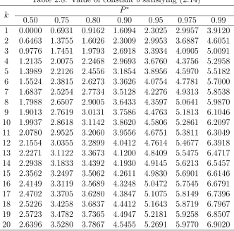
known as theleast favorable configuration (LFC). Next, supposeb is a constant satisfying
P∗ =
Z b
−∞ · · ·
Z b
−∞ |Σ|12
(2π)k2
exp
−y 0Σ−1y
2
dy1· · ·dyk. (1.27)
according to the partition rule (1.24), we have
P[CD]>P∗, ∀ µ∈Rk+1, σ∈R+.
The values of design constantbhave been tabulated in the Table 1 of Tong (1969). For the unknown σ2 case, Tong (1969) also constructed a two-stage and a purely sequential
procedure. For the unknown σ2 case, Datta and Mukhopadhyay (1998) had constructed a fine-tuned purely sequential procedure and some other multistage methodologies,
em-phasizing the second-order asymptotic properties. However, the sequential procedures
are known to be operationally inconvenient and rather cumbersome to use, as decisions
and computations need to be carried out after each stage of the sampling process. With
that as the motivation, Solanky (2006) constructed a two-stage procedure with
elimina-tion which eliminates too inferior or too superior populaelimina-tions after the stage one of the
sampling process and in the stage two sampling is carried out only from the competing
2
Partition Problem for Exponential
Distributions
In the chapter 1, the method of partitioning a set of normal populations respect to the
location parameter was introduced. However, what about the case when the populations
needed partitioning are not following a normal distribution? For example, suppose
sev-eral new developed medicine needs to be classified as “Good” and “Bad” based on the
effectiveness compared a control medicine. Or, several different brand light bulbs need
partitioning according to their lifetime compared to a standard bulb. In these cases, the
populations will probably be distributed as two-parameter exponential distribution, and
will require methodology to partition two-parameter exponential distributions with
re-garding to a control. In this chapter, a procedure of partitioning several two-parameter
exponential distributions respect to their location parameter is introduced. The first few
sections show the logical thinking and derivation of design parameters for this problem,
including a detailed discussion on existence and derivation of the Least Favorable
con-figuration. The later part of the chapter is devoted to developing first and second order
2.1 Formulation for Partitioning Two-parameter
Exponential Distributions
In this section, we will introduce the formulation of partition problem for two-parameter
exponential distributions respect to the location parameter along with the setting of
Bech-hofer’s (1954) indifference zone idea and give some necessary notations of some statistical
symbols for later sections’ use.
It is assume that there are (k + 1) independent negative exponential populations
π0, π1, . . . , πk, with unknown location parameters θ, i = 0,1, . . . , k, and common scale
parameterσ. π1, . . . , πkare denoted as the populations to be partitioned andπ0 is denoted
as the standard or control populations. For i = 0, . . . , k, the density function of the
population is expressed as
fX(xij) =σ−1exp{−(xij −θi)/σ}I(xij > θi). (2.1)
Given arbitrary but fixed constants δ1 and δ2, let us define three subsets along the
lines of the Bechhofer’s (1954) indifference zone formulation as
ΩB = {πi :θi ≤θ0+δ1, i= 1, ..., k},
ΩI = {πi :θ0+δ1 < θi < θ0 +δ2, i= 1, ..., k},
ΩG = {πi :θi ≥θ0+δ2, i= 1, ..., k}.
(2.2)
We refer to ΩGas the set of “good populations” and ΩBas the set of “bad populations”.
It is important to note that the choice of the constants δ1 and δ2 is generally determined
by the experimenters based on the prior knowledge of the practical situation. Our aim
is to correctly partition the populations into two groups. The subset ΩI is considered
of the populations belonging to this set. Next, with high accuracy, we want to partition
the set Ω into two disjoint subsets SB and SG, such that, ΩB ⊆ SB and ΩG ⊆ SG.
Such a partition can guarantee that all true “good population” and “bad population”
are correctly labeled, which is known in the literature as a correct decision(CD). In other
words, given a preassigned value P∗, 2−k < P∗ <1, we seek statistical methodologies ℘
to determineSB and SG, such that
P{CD|θ, σ, ℘} ≥P∗ ∀ θ ∈Rk+1, σ ∈R+, (2.3)
where θ= (θ0, θ1,· · · , θk)0.
Alone with the setting originated in Tong (1969), with N observations from each of
the k populations to be partitioned and the control population, we define a partition rule
℘ was defined as:
SB = {πi :Ti−T0 < d, i= 1,· · · , k},
SG = {πi :Ti−T0 > d, i= 1,· · · , k},
(2.4)
where Ti = M in1≤j≤N{Xi1, . . . , XiN} is a point estimator of θi, i = 0,1,· · · , k. Through
this decision rule, the probability of correct partition is controlled by the selection size.
Or equivalently, the power of grouping procedure according the the rule ℘ is controlled
by the setting of collection size of the k + 1 populations. Next we will show how this
relationship takes effect. In order to make the derivation clear, the following are defined
for later use:
d= (δ1+δ2)/2, a= (−δ1+δ2)/2, λ=σ/a, and
m =
k/2 if k is even,
(k+ 1)/2 if k is odd.
(2.5)
exponential populations are partitioned based on rule ℘. Then the probability of making
a correct decision(ΩB ⊆SB,ΩG ⊆SG) can be obtained as
P(CD|σ, ℘) =P[Ti−T0 < d, Tj −T0 > d,0≤i≤N1,0≤j ≤N2|σ, ℘]. (2.6)
Where N1 is the number of populations in ΩB and N2 is the number of populations
in ΩG. Since the population location parameters are unknown, in order to guarantee
(2.1.3) to hold, the infimum of the left hand side should be controlled greater or equal
to P∗. Holding this purpose, the least favorable configuration of the population location
parameters(LFC) θ0 amongRk+1 minimizing the probability of correct partition is being
analyzed here. In other words, we are interested in finding the worst or hardest situation
to do the partition process.
The above states the importance of detecting the LFC to the partition process. Next
we try to tackle the task of finding the LFC.
Theorem 2.1.1 If a vector θ0 is a least favorable configuration under under procedure
℘, it has to satisfy the two conditions below: (i) ΩI is empty.
(ii) All populations that needs to be partitioned have a location parameter lying on the boundaries which are either θ0+δ1 or θ0+δ2.
Proof: Suppose there is a parameter configurationθ1 which satisfies that Ω
Iis not empty
and the PCD of it can be expressed as (2.6). Thenk−N1−N2 >0 and there always exits
another parameter configuration which is more difficult to be partitioned. For example,
let us assume a configuration θ2 that k−N
configuration θ2 can be expressed as
P(CD|θ2, σ, ℘)
= P[Ti−T0 < d, Tj −T0 > d, Tl−T0 < d,0≤i≤N1,0≤j ≤N2,
0≤l ≤k−N1−N2|σ, ℘]
= P[Ti−T0 < d, Tj −T0 > d∩Tl−T0 < d]
= P[Ti−T0 < d, Tj −T0 > d]·P[Tl−T0 < d|Ti−T0 < d, Tj−T0 > d]
< P[Ti−T0 < d, Tj −T0 > d] =P[CD|θ1, σ, ℘].
Compared to the case above, next a case that not all populations’ location parameter are
on the boundary of the indifference set is discussed.
Under the setting of (i) suppose there is a parameter configuration θ3 which satisfies that ΩI is empty and the PCD of it can be expressed as (2.6). So now k−N1−N2 = 0.
Let θi = θ0+δ1+τi, θj =θ0+δ2+τj, τi, τj ≥ 0 for i= 0, . . . , N1 and j = 0, . . . , N2 be
assumed as the real setting of components. Then the PCD under configuration θ3 can be
expressed as
P
h
CD|θ3, σ; ℘
i
= PhTi−T0 < d, Tj−T0 > d, 0< i≤N1, 0< j ≤N2|θ3, σ
i
= PhTi−θi
σ/n −
T0−θ0
σ/n <
d−θi+θ0
σ/n ,
Tj−θj
σ/n −
T0−θ0
σ/n >
d−θj+θ0
σ/n ,
0≤i≤N1, 0≤j ≤N2
i
= PhZi−Z0 <
d−(δ1−τi)
σ/n , Zj−Z0 >
d−(δ2 +τj)
σ/n , 0≤i≤N1, 0≤j ≤N2
i
= PhZi−Z0 <
a σ/n +
τi
σ/n, Zj−Z0 >− a σ/n−
τj
σ/n, 0≤i≤N1, 0≤j ≤N2
i
= PhZi−Z0 <
an
σ +
τin
σ , Z0−Zj < an
σ +
τjn
σ , 0≤i≤N1, 0≤j ≤N2
i
≤ PhZi−Z0 <
an
σ , Z0−Zj < an
σ , 0≤i≤N1, 0≤j ≤N2
i
It can be shown that the infimum of PCD under configuration θ3 is attached when
τi, τj = 0 fori = 0, . . . , N1 and j = 0, . . . , N2. Equivalently speaking, the infimum is
at-tached when all populations have a location parameter on the boundary of the indifference
zone.
Next, under the setting of conditions from Theorem 2.1.1, suppose out ofkpopulations
there are r exponential populations having a location parameter at θi =θ0+δ1,0≤i≤r
and k−r exponential populations having a location parameter atθj =θ0+δ2, r > j ≤k.
Here comes a goal that we need to find the value of r(0 ≤ r ≤ k) which leads the
probability of the correct decision to attach the infimum.
Without the loss of generality assume that the first r populations have the location
parameterθ0+δ1and the restk−rpopulations have the location parameterθ0+δ2.
Denot-ing this configuration as θ0(r), then the probability of correct decision can be expressed
as
PhCD|θ0(r), σ; ℘i
= PhTi−T0 < d, Tj−T0 > d, 0< i≤r, r < j≤k|θ0(r), σ
i
= PhTi −θi
σ/n −
T0 −θ0
σ/n <
d−θi+θ0
σ/n ,
Tj−θj
σ/n −
T0−θ0
σ/n >
d−θj+θ0
σ/n ,
1≤i≤r, r+ 1 ≤j ≤ki
= PhZi−Z0 <
d−δ1
σ/n , Zj −Z0 >
d−δ2
σ/n , 1≤i≤r, r+ 1 ≤j ≤k
i
= PhZi−Z0 <
an
σ , Z0−Zj < an
σ , 1≤i≤r, r+ 1≤j ≤k
i
, (2.7)
where Zi = Tσ/ni−θi for i = 0, . . . , k, are all following standard exponential distributions.
According the (1.19),
F(Z) =P(Z ≤z) = P(Tσ/n−θ ≤z)
=P(T ≤ zσ
n +θ) = 1−e
−n(zσn+θ−θ) σ
= 1−e−z.
Then fZ(z) = [F(Z)]
0
= e−z, which is the density function of standard exponential
distribution.
Let us define Yi = Zi −Z0 for 0 < i ≤ r and Yi = Z0 −Zi for r < i ≤ k , then Yi for i = 1, . . . , k are all following Laplace distribution. Then it can be obtained that
Y = (Y1, Y2, . . . , Yk)
0
is a joint distribution of k Laplace distributions. And the (k×k)
covariance matrix ΣY = (σij) as
σij =
2 for i=j,
1 for i6=j,andi, j ∈[1, r] ori, j ∈ [r+ 1, k],
−1 for i6=j,andi∈[1, r] andj ∈ [r+ 1, k].
(2.8)
Then probability of of correct decision (2.7) can be considered as a probability related to a multivariate distribution. Let us denote the density function of Y as a multivariate
distribution expressed as fY(·).
Next, we will investigate if the multivariate distributionfY(·) is a Multivariate Laplace
distribution. And it is important to note that a multivariate Laplace distribution is not
a unique distribution. Also, using (2.7), we will next investigate the value ofr which will
minimize the probability requirement from (2.7). This choice of r, known as LFC in the
statistical literature, will have that at a given fixed significance level α
PhCD|θ0(r), σi ≥P∗
After the value of r is identified, some critical constant related to n can be computed
correspondingly. That will help statisticians with determining the sample size needed if
the power of partition procedure is required. These two different directions are detailed
discussed in the later sections.
2.2 Multivariate Distribution Identification
In the last section, a multivariate distribution is derived based on the form of the
proba-bility expression of the correct decision. In this section, the statement that distribution of
Y is a Multivariate Laplace distribution is verified. In case the statement is true, as was
the case in Tong (1969), formula of probability of correct decision (2.7) can be evaluated as a integral of a Multivariate Laplace distribution, which is somewhat easy to solve with
or without standard software packages. In addition, some good properties of Multivariate
Laplace distribution can be developed related to our problem and then used to identify
the LFC (Least Favorable Configuration).
It is known that the joint distribution of k normal variables is not guaranteed to
follow a Multivariate Normal distribution. The Multivariate distribution requires that any
linear combination of its components to follow the same type of marginal distribution.
For example, a multivariate density is known as a multivariate normal density if any
linear combination of its components also follows a normal density. The realization of
this condition is the reason why Tong could derive a multivariate normal distribution for
the partition problem respect a set of normal populations in Tong (1969). However, the
multivariate Laplace distribution doesn’t follow the same properties. Next, we show how
a multivariate normal variable can be derived from normal partition problem and why
the multivariate Laplace variable can not, under the partition problem considered in this
Theorem 2.2.1 SupposeZ0, Z1, Z2 are independent standard normal variables and Y1 =
Z1−Z0 and Y2 =Z2−Z0, then the joint distribution of Y1 and Y2 is a bivariate normal
distribution
Proof: Note that in probability theory and statistics, the multivariate normal
distribu-tion is a generalizadistribu-tion of the one-dimensional normal distribudistribu-tion to higher dimensions.
One definition is that a random vector is said to be k-variate normally distributed if every
linear combination of its k components has a univariate normal distribution. Therefore,
to prove the joint distribution ofY1 andY2 is not a bivariate normal distribution is
equiv-alent to show that any linear combination ofY1 and Y2 is following a normal distribution
is wrong. Now we try to find whether the distribution ofaY1+bY2 is normal distribution
when a and b are not both 0. Let us define
X =aY1+bY2 =aZ1+bZ2 −(a+b)Z0.
So the expectation and variance of X can be obtained
E[X] =aE[Z1] +bE[Z2]−(a+b)E[Z0] = 0
V ar[X] =a2V ar[Z1] +b2V ar[Z2] + (a+b)2V ar[Z0] = 2(a2+ab+b2),
To find the distribution ofX, we first find the joint distribution of (X1 X2 X)0 by the
method of transformation of variables. Then, derive the distribution of X by obtaining
the marginal distribution. Here we let X1 = Z1 and X2 = Z2. Since Z0, Z1, Z2 are
independent normal variables. then the joint density ofZ0, Z1, Z2 can be expressed as
f(Z1, Z2, Z0) = (2π)−
3 2e−
1 2(z
2
And the relationship of Z0, Z1, Z2 and X, X1, X2 is
Z1 = X1
Z2 = X2
Z0 = a+abX1+a+bbX2−a+1bX
J =
1 0 0
0 1 0
a a+b
b a+b −
1
a+b
=− 1
a+b.
Then the joint density function of (X1 X2 X)0 can be obtained as
g(x1, x2, x) = (2π)−
3 2e −1 2 h x2
1+x22+(aa+bx1+ b a+bx2−
1
a+bx)
2
i
· |J|
= (2π)−32e −12
h
x2 1+x22+
a2
(a+b)2x 2 1+
b2
(a+b)2x 2 2+
1 (a+b)2x
2+ 2ab
(a+b)2x1x− 2a
(a+b)2x1x− 2b
(a+b)2x2x
i
· | 1 a+b|
= (2π) −3
2 |a+b|e
−1 2
h
2a2+2ab+b2
(a+b)2 x 2 1+
2ab
(a+b)2)x1x2− 2a
(a+b)2x1x
i
e− 1 2
h
a2+2ab+2b2
(a+b)2 x 2 2−
2b
(a+b)2x2x
i
e− 1 2(a+b)2x
2 .
Then the marginal density g(x2, x) can be solved as
g(x2, x) =
Z ∞
−∞
g(x1, x2, x)dx1
= (2π) −3
2 |a+b|e
−1 2
h
a2+2ab+b2
(a+b)2 x 2 2−
2b
(a+b)2x2x
i
e− 1 2(a+b)2x
2
·
Z ∞
−∞ e−
2a2+2ab+2b2
2(a+b)2
h
(x1−
ax−abx2
2a2+2ab+b2)
2−( ax−abx2 2a2+2ab+b2)
2
i
dx1.
Let us make the part of g(x2, x) as
A=
Z ∞
−∞ e−
2a2+2ab+2b2
2(a+b)2
h
(x1− ax
−abx2 2a2+2ab+b2)2−(
ax−abx2 2a2+2ab+b2)2
i
dx1
=e
(ax−abx2)2
2(a+b)2(2a2+2ab+b2)
Z ∞
−∞ e−
(x1− ax−abx2
2a2+2ab+b2)2
2(a+b)2/(2a2+2ab+b2)dx
1
=e
(ax−abx2)2
2(a+b)2(2a2+2ab+b2) ·
h 2π(a+b)2
2a2+ 2ab+b2
i(−12)(−1)
=h 2π(a+b)
2
2a2+ 2ab+b2
i12
e
a2b2x22−2a2bx2x+a2x2
Then the density of (X2, X) can be simplified as
g(x2, x) =
(2π)−32 |a+b|e
−1 2
h
a2+2ab+b2
(a+b)2 x 2
2−(a+2bb)2x2x
i
e− 1 2(a+b)2x
2
·h 2π(a+b)
2
2a2+ 2ab+b2
i12
e
a2b2x22−2a2bx2x+a2x2
2(a+b)2(2a2+2ab+b2)
= (2π)
−1
(2a2+ 2ab+b2)12e
− 1 2(a+b)2x
2
·e−
1
2(a+b)2(2a2+2ab+b2)
h
(a2+2ab+2b2)(2a2+2ab+b2)x22−2b(2a2+2ab+b2)x2x−a2b2x22+2a2bx2x−a2x2
i
= (2π)
−1
(2a2+ 2ab+b2)12e
− 1 2(a+b)2x
2 e
a2
2(a+b)2(2a2+2ab+b2)x2
·e−
1
2(a+b)2(2a2+2ab+b2)
h
2(a+b)2(a2+ab+b2)x22−2b(a+b)2x2x
i
= (2π)
−1
(2a2+ 2ab+b2)12e
− 1 2(a+b)2x
2 e
a2
2(a+b)2(2a2+2ab+b2)x
2 e−
a2+ab+b2
2a2+2ab+b2
h
x22−a2+bxab+b2x2
i
,
then solve g(x) by solving
g(x) =
Z ∞
−∞
g(x2, x)dx2
= (2π)
−1
(2a2+ 2ab+b2)12 e−
1 2(a+b)2x
2 e
a2
2(a+b)2(2a2+2ab+b2)x
2Z ∞
−∞ e−
a2+ab+b2
2a2+2ab+b2
h
x2 2−
bx a2+ab+b2x2
i
dx2.
Similarly, we can let part ofg(x) be
B =
Z ∞
−∞ e−
a2+ab+b2
2a2+2ab+b2
h
x22−a2+bxab+b2x2
i dx2 = Z ∞ −∞ e−
a2+ab+b2
2a2+2ab+b2
h
(x2− bx 2(a2+ab+b2))
2−( bx
2(a2+ab+b2))
2
i
dx2
=e
b2x2
4(2a2+2ab+b2)(a2+ab+b2)
Z ∞
−∞ e−
(x2− 1 2bx
a2+ab+b2)2 (2a2+2ab+b2)/(a2+ab+b2)dx
2
=e
b2x2
4(2a2+2ab+b2)(a2+ab+b2) ·
h
2π·2(2a2+ 2ab+b2)/(a2+ab+b2)
i(−12)(−1)
=h4π(2a
2+ 2ab+b2)
a2+ab+b2
i12
e
b2x2
then the density function of variableX can be obtained as
g(x) = (2π) −1
(2a2+ 2ab+b2)12 e−
1 2(a+b)2x
2 e
a2
2(a+b)2(2a2+2ab+b2)x
2
·h4π(2a
2+ 2ab+b2)
a2+ab+b2
i12
·e
b2x2
4(2a2+2ab+b2)(a2+ab+b2)
=h4π(a2+ab+b2)i −1
2
·e−
1
4(a+b)2(2a2+2ab+b2)(a2+ab+b2)
h
2(2a2+2ab+b2)(a2+ab+b2)x2−2a2(a2+ab+b2)x2−b2(a+b)2x2
i
=
h
4π(a2+ab+b2)
i−12
e−
1
4(a+b)2(2a2+2ab+b2)(a2+ab+b2)
h
(2a2+2ab+b2)(a+b)2x2
i
=h4π(a2+ab+b2)i −1
2 e−
x2
4(a2+ab+b2).
It is shown that g(x) is density function of a normal distribution with µx = 0 and
σ2
x = 2(a2 +ab+b2). It implies X = aY1 +bY2 follows normal distribution when a and
b are not both 0. That is, the joint distribution of Y1 and Y2 is a multivariate normal
distribution.
Above, we have shown that for the normal partition problem considered in Tong
(1969), a Multivariate Normal distribution can be derived to calculate the probability of
correct decision. Next, we show some results for the case of partitioning two-parameter
exponential distributions.
Theorem 2.2.2 Suppose Z0, Z1, Z2 are independent standard exponential variables and
Y1 =Z1−Z0 andY2 =Z2−Z0, then the joint distribution of Y1 andY2 is not a bivariate
Laplace distribution.
Proof: Since Z0, Z1, Z2 are independent standard exponential variables, Y1, Y2 are both
following Laplace distribution with location parameter of zero and scale parameter of 1.
Then note that to prove the joint distribution of Y1 and Y2 is not a bivariate Laplace
Laplace distribution. That is, we will prove that the distribution of aY1 + bY2 is not
Laplace distribution. Let us define
X =aY1+bY2 =aZ1+bZ2−(a+b)Z0 (2.10)
SoE[X] =aE[Z1] +bE[X2]−(a+b)E[Z0] = 0. And then denote X =A−B, where
A = aZ1+bZ2
B = (a+b)Z0.
Let us consider the case thata andb are both positive but not equal for simplicity. First,
since Z0, Z1, Z2 are independent exponential variables, then the characteristic function of
A is
ϕ(A) =ϕ(aZ1)·ϕ(bZ2) =
1 1−iat ·
1 a−ibt.
Since a6=b, then the characteristic function can be expressed as
ϕ(A) = a a−b ·
1 1−iat +
b b−a ·
1 1−ibt.
By inverse Fourier transform, it is easy to obtain the density function of A and B, which
are expressed as
f(A) = a−ab · 1
ae −A
a + b
b−a·
1
be −A
b = 1
a−be −A
a + 1
b−ae −A
b, 0≤A <∞
f(B) = a+1be−aB+b, 0≤B <∞.
Then to solve then cumulative function of X,
P(X ≤x) =P(A−B ≤x)