* Corresponding author. Tel./fax: +98-21-77240481
E-mail addresses: [email protected](M. Moshref Javadi), © 2011 Growing Science Ltd. All rights reserved.
doi: 10.5267/j.ijiec.2010.03.007
Contents lists available atGrowingScience
International Journal of Industrial Engineering Computations
homepage: www.GrowingScience.com/ijiec
Supplier selection and order lot sizing using dynamic programming
M. M. Moqria, M. Moshref Javadia*and S. A. Yazdiana
a
Department of Industrial Engineering, Iran University of Science and Technology, Narmak, Tehran Iran
A R T I C L E I N F O A B S T R A C T
Article history: Received 10 January 2010 Received in revised form 10 June 2010
Accepted 26 June 2010 Available online 27 June 2010
In this paper, we consider a multi-period integrated supplier selection and order lot sizing problem where a single buyer plans to purchase a single product in multiple periods from several qualified suppliers who are able to provide the required product with the needed quality in a timely manner. Product price and order cost differs among different suppliers. Buyer’s demand for the product is deterministic and varies for different time periods. The problem is to determine how much product from which supplier must be ordered in each period such that buyer’s demand is satisfied without violating some side constraints. We have developed a mathematical programming model to deal with this problem, and proposed a forward dynamic programming approach to obtain optimal solutions in reasonable amount of time even for large scale problems. Finally, a numerical example is conducted in which solutions obtained from the proposed dynamic programming algorithm is compared with solutions from the branch-and-bound algorithm. Through the numerical example we have shown the efficiency of our algorithm.
©2011 Growing Science Ltd. All rights reserved.
Keywords: Supply chain Supplier selection Order lot sizing Dynamic programming Wagner Whitin
1. Introduction
literature. Order lot-sizing is among the most important problems in this domain. In these types of problems inventory holding costs and fixed ordering costs are included in the mathematical model. The smaller the batch size is, due to increase in number of yearly orders, the greater the ordering cost will be. There have been little works in the SSOLSP domain to simultaneously consider the supplier selection and inventory control. Therefore, the problem is to consider the most appropriate suppliers, and to determine the optimal lot-size for each product in each planning period to minimize the total inventory holding costs.
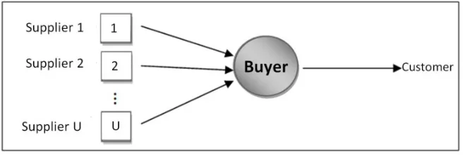
Fig. 1 General scheme of the problem under consideration
Brahimi et al. (2006) presented a comprehensive review of the lot sizing problem in the case that demand of the product varies over different time periods. These types of problems were first
proposed in Wagner and Whitin (1958) and was solved using dynamic programming in O(n2). Later,
Evans (1985), Heady and Zhu (1994) and others improved the solution procedure proposed by Wagner and Whitin (1958). Due to applicability of the problem, many other researchers such as Aryanezhad(1992), Wolsey(1995), and Cattrysse et al.(1990) worked on the other aspects of this problem. The supplier selection problem without inventory consideration was also studied in the literature (Current and Weber (1994)). However, there are limited efforts for the case of multiple suppliers where inventory is also considered. Aissaoui et al. (2007) dedicated a review paper for this problem for different cases. Dai and Qi (2007), and Rosenblatt et al. (1998) examined this problem where the demand of the product was constant and developed the well known economic order quantity method for this problem. Tempelmeier (2002) considered a lot-sizing problem with single product and proposed a new model formulation with discount rate along with a heuristic solution method for this problem where demand of the product varies over different periods. Their proposed solution procedure yielded near optimal solutions. Ustun and Demirtas (2008a and 2008b) tackled the problem using multiple criteria decision making techniques. Rezaei and Davoodi (2006 and 2008) considered a multi-product problem under fuzzy environment and with the undesirable product quality, respectively, and solved the developed problem using genetic algorithm (GA) method. Hassini (2008) also considered the limited capacity of suppliers and proposed a linear programming model for the problem when discount rate and due date were part of the modeling formulation. In this problem, decisions regarding mode of transporting the product can also be considered simultaneously and it requires a more sophisticated model (Liao and Rittscher(2007)). Basnet and Leung (2005) considered the supplier selection and order lot sizing problem in the case where there were multiple products each with different deterministic demand. They developed an integer linear programming (ILP) formulation for the problem and proposed a heuristic algorithm to solve the model. The proposed method of this paper is based on the approach which was originally developed by Basnet and Leung (2005) for a single product. Sadjadi et al. (2009) developed the Wagner Within algorithm for economic lot sizing problems based on the planning horizon theorem and the economic part period concept. This problem was investigated both when backlogging, inventory holding and setup costs were fixed and unfixed.
propose a new mathematical relation using dynamic programming to find the optimal solution. The solution procedure for the proposed algorithm is presented both in a step-by-step manner and tabular computations. Computational results along with comparisons with the branch-and-bound solution procedure for a hypothetical numerical example are summarized in Section 4. Finally, in Section 5 conclusions are given.
2. Problem description and the mathematical formulation
Consider Fig. 1 where a producer (buyer) can purchase its required item (product) from different suppliers. Each supplier has a different unit price for the product; and, in addition, each has a different fixed ordering cost. Buyer’s demand in each period is deterministic and is known in advance. If the lot size for a period exceeds buyer’s demand for that period, excessive products are held in inventory to use in subsequent periods. However, no backlog is permitted. The buyer needs to make decisions on how much product must be ordered from each supplier in each period.
We assume that:
• Products are shipped directly from suppliers to the buyer (i.e., there is no intermediate distributer);
• Only one product is considered;
• Suppliers’ capacity is unlimited;
• Buyer’s demand for the product is deterministic and is known in advance;
• The planning horizon is finite (1,2,…,T);
• Product price does not depend on the amount of product ordered (i.e., there is no discount
rate);
• Inventory holding cost is linearly proportional to the amount of product stocked in inventory;
• Order lead-time is deterministic and is the same for each period (here, we assume it to be
zero);
• Initial inventory of the first period and the inventory at the end of the last period are assumed
to be zero;
• No product shortage is permitted (i.e., the buyer’s demand for the product in each period
should be satisfied).
Sets, parameters and decision variables are defined as follows:
U Index of suppliers, u=1,2,…,U,
T Index of time periods, t=1,2,…,T,
dt Buyer’s demand for the product in period t,
ht Unit inventory holding cost in period t,
sut Fixed ordering cost from supplier u in period t,
put Unit product price of supplier u in period t,
It Inventory at the end of period t,
Xut Amount of product ordered (lot size) from supplier u in period t,
Yut Equals 1 if the buyer orders from supplier u in period t, and 0 otherwise.
Minimize
T
(1)
= + (2)
, (3)
0 or 1 , (4)
, 0 , (5)
The objective function (1) minimizes total costs, composed of fixed ordering cost, variable purchasing cost and inventory holding cost. Constraint set (2) is the flow conservation equation in
each period t. Constraint set (3) correlates the amount of product ordered from supplier u in period t
to the binary variable Yut. This constraint causes Yut to be 1 in those periods that Xut is positive which
means ordering is performed. Finally, constraints (4) and (5) are binary and non-negativity constraint, respectively. Before presenting the solution procedure, we first describe some characteristics of the optimal solution.
Lemma 1. Given suppliers have unlimited capacity, purchasing from different suppliers in each single period cannot be optimal. In other words:
Xut Xkt = 0 t, u≠k
Lemma 2. For every u and t in the optimal solution we have XutIt-1=0. This means that in each period
either an order is placed or we have inventory from the preceding period.
Proof. Proofs of the two above lemmas, for multi-product problems, are given in Basnet and Leung (2005).
Theorem 1. In the optimal solution if Xut >0, then Xut=∑ for a k>0, which means in every period
t the lot size must be equal to the sum of buyer’s demand in k+1 consecutive periods beginning from
period t.
Proof. The proof is obtained directly from lemma 1 (Basnet and Leung, 2005).
Theorem 2. Assume in the optimal solution we have It = 0 for some t, then we can plan for periods 1
through t-1, and t through T, independently.
Proof. Wagner and Whitin(1958) proposed this theorem for a single supplier case, and using theorem 1 showed that this theorem also holds for a multiple supplier case.
Using the above theorems, Wagner and Whitin (1958) proposed the following relation (in the single-sourcing case) for planning with minimum cost:
( ) min min ( ) , ( )
t 1 t
j l k t
1 j t
l j k n 1
F t s h d F j 1 s F t 1
−
≤ ≤ = = +
⎧ ⎛ ⎞ ⎫
⎪ ⎜ ⎟
= ⎨ + + − + − ⎬
⎜ ⎟ ⎭
⎪ ⎝ ⎠
⎩
∑ ∑
where F(0)=0 and F(1) =s1. Using this relation, by having minimum costs of previous periods in
hand, we can calculate the minimum cost in the beginning of period t.
Assume that in all periods the product price is the same. Therefore, using Eq. (6) and theorems (1) and (2) we can define a new relation for the multi-sourcing case.
(
)
( ) min min min ( ) , min ( )
t 1 t
uj n k ut
1 j t 1 u U 1 u U
n j k n 1
F t s h d F j 1 s F t 1
− ≤ ≤ ≤ ≤ ≤ ≤ = = + ⎧ ⎡ ⎛ ⎞⎤ ⎫ ⎪ ⎢ ⎜ ⎟⎥ ⎪ = ⎨ + + − + − ⎬ ⎜ ⎟ ⎢ ⎥ ⎪ ⎣ ⎝ ⎠⎦ ⎪ ⎩
∑ ∑
⎭ (7)where F(0)=0 and F(1)= min . In general, where the product price varies in different periods, we
have:
(
)
( ) min min min ( ) , min ( )
t 1 t t
uj n k uj l ut
1 j t 1 u U 1 u U
n j k n 1 l j
F t s h d p d F j 1 s F t 1
− ≤ ≤ ≤ ≤ ≤ ≤ = = + = ⎧ ⎡ ⎛ ⎛ ⎞ ⎞⎤ ⎫ ⎪ ⎢ ⎜ ⎜ ⎟ ⎟⎥ ⎪ = ⎨ ⎢ ⎜ + + ⎜ ⎟+ − ⎟⎥ + − ⎬ ⎪ ⎣ ⎝ ⎝ ⎠ ⎠⎦ ⎪ ⎩
∑ ∑
∑
⎭ . (8)Note that Eq. (8) calculates the minimum total cost for the first t periods. If in the optimal policy the
last order takes place in the last period, we have,
(
( ))
min )
(t s p d F t 1
F ut ut t
U u
1 + + −
=
≤
≤ (9)
otherwise,
( ) min min ( )
t 1 t t
uj n k uj l
1 j t 1 u U
n j k n 1 l j
F t s h d p d F j 1
− ≤ ≤ ≤ ≤ = = + = ⎧ ⎡ ⎛ ⎛ ⎞ ⎞⎤⎫ ⎪ ⎢ ⎜ ⎜ ⎟ ⎟⎥⎪ =⎨ + + + − ⎬ ⎥ ⎟ ⎜ ⎜ ⎟ ⎢ ⎪ ⎣ ⎝ ⎝ ⎠ ⎠⎦⎪ ⎩
∑ ∑
∑
⎭ . (10)Eq. (9), determines the minimum ordering cost from different suppliers in period t. In Eq. (10) we
consider different cases for the last order period. Assume that the last period in which an order is placed is j, then the least cost associated with this policy is as follows,
⎜⎜ ⎜ ⎝ ⎛ ⎟⎟ ⎟ ⎠ ⎞ − + ⎟ ⎟ ⎠ ⎞ ⎜ ⎜ ⎝ ⎛ + +
∑ ∑
∑
− = = + = ≤ ≤ 1 t j n t 1 n k t j l l uj k n uj U u1min s h d p d F(j 1) . (11)
Eq. (11) is composed of two parts; the first part determines which supplier satisfies sum of demands
from period j through period t with the least cost, and 1 is the least cost for meeting the
demands of the first j-1 periods. Therefore, if the last period in which an order is placed becomes j,
Eq. (11) yields the minimum cost for the entire planning horizon. Since the Eq. (8) is recursive we can use the dynamic programming technique to solve the problem.
3.Dynamic programming algorithm
For every period t* (t*=1,2,…,T), the following algorithm gives the least cost for meeting the demand
of the product up to the period t*.
1. For every period t** (t**=1, 2, …, t*), and for every u (u=1, 2, …, U), consider a case in
which the last order is placed in period t** on supplier u, and demands of periods preceding
period t** are satisfied with the least cost (this minimum cost is obtained in previous stages).
2. Among t*×u different policies, select that policy which has the least cost. This is the optimal
policy to satisfy demands from period 1 through t*.
3. If t*=T, then the algorithm is terminated, or else, repeat steps 1 and 2 for t*+1.
One important advantage of the proposed algorithm is that the search space is reduced from UT to
T(T+1)/2*U in order to obtain the optimal solution. Wagner and Whitin (1958) presented the
following tabular calculations for their algorithm (with a single supplier):
Table 1
Tabular calculations for Wagner-Whitin algorithm
1 2 3 4 N
1 1 (1)2 (1,2)3 (1,2,3)4 … (1,2,..., N- 1)N
2 12 (1)23 (1,2)34 … (1,2,..., N-2)N- 1,N
3 123 (1)234 … (1,2,...,N-3)N-2,N- 1,N
4 1234 …
Min (1) (1,2) (1,2,3) (1,2,3,4) (1,2,…,N)
In Table 1, columns represent different planning periods, and the last row in each column is the least
cost in the optimal solution up to the current period. The expression (1, 2, …, t**) t**+1, t**+2, …,
t* is the planning for first t* periods and shows the policy in which the last order is placed in period
t**+1 and the first t** periods are planned optimally. In this table, calculations are started with the
first column then the second column, and so forth (forward planning). When calculations of the tth
column are completed we have the optimal ordering plan to meet all the demands up to period t.
Finally, in column N, we can obtain the optimal plan of the entire planning period in which the last
row shows the optimal total cost. An example of tabular calculations for the proposed algorithm with two suppliers is depicted in Fig 2.
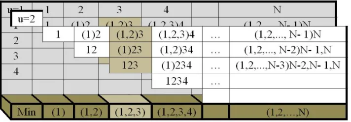
Fig. 2: Tabular calculations of the proposed algorithm
For the sake of simplicity, in Fig. 2 we have just considered two suppliers. In table 2, different layers
of u represent different suppliers. In each layer, u is calculated the same as in Wagner-Whitin tabular
calculations in case of one supplier (supplier u). The main difference between our method and the
Wanger-Whitin method is in calcualtions of the last row (the “Min” row). As it can be seen from Fig
2, for all different layers (suppliers), we have only one common last row. The value of the t*th
write the minimum value of that cell over all layers. For example, mu[(1)23] is the minimum value of (1)23 over all layers.
Table 2
Development of Table 1 in the case of multiple supplires.
{u}
1 2 3 4 N
1 mu[1] mu[(1)2] mu[(1,2)3] mu[(1,2,3)4] … mu[(1,2,..., n- 1)n]
2 mu[12] mu[(1)23] mu[(1,2)34] … mu[(1,2,..., n-2)n- 1,n]
3 mu[123] mu[(1)234] … mu[(1,2,...,n-3)n-2,n-1,n]
4 mu[1234] …
min (1) (1,2) (1,2,3) (1,2,3,4) mu[(1,2,…,n)]
Calcualtions in this table are also started with the first column and they continue column-by-column. Initially, claculations of the first column for every layer is executed and then the least cost of the
column is written in the last row (common between all layers) of the table. Similarly, for the tth
column, using the common last row, we perform calculations for each layer, and then the least cost of this column over all layers is written in the last row of the tth column.
4.Computational Results
A hypothetical example with four planning periods and two suppliers is considered in this section. Parameters of this numerical example are presented in Table 3. For the ease of calculations, we assume that inventory holding cost per unit per unit time is constant over all periods and is equal to 1.
Table 3
Parameters of the numerical example
T dt It s1t p1t s2t p2t
1 30 1 50 2 70 2.5
2 35 1 45 2.5 75 2
3 40 1 60 3 80 2.5
4 20 1 60 3 80 2
110+45+2.5*(35+40)+1*40=382.5. 3. An order is placed in period 1 to satisfy all the damands of periods 1 through 3 with the total cost of 50+2*(30+35+40)+(1*35)+(1+1)*40=375. The minimum of 395, 382.5 and 375 is written in the last row. Similarly, for the column 4 the least cost is 472.5 which corresponds to the policy in which an order is placed to satisfy all the demands of periods 2 through 4, and the demand of period 1 is ordered in the first period. This is the optimal ordering policy over four periods.
Table 4
Results of the numerical example addressed by Wagner and Whitin (1958) (supplier 1)
1 2 3 4
1 110 242.5 395 495
2 215 382.5 465
3 375 472.5
4 475
Min 110 215 375 472.5
Table 5
Results of the numerical example for supplier 2.
1 2 3 4
1 140 255 395 495
2 292.5 375 465
3 395 455
4 557.5
Min 140 255 375 455
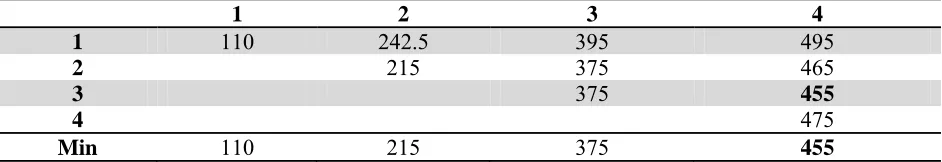
Now consider a case where there are two suppliers. The value in cell (1,1) for supplier 1 is 50+2*30=110 (Table 4), and for supplier 2 is 70+2.5*30=140 (Table 5). Thus, mu[1]=110; and, therefore, the value of the last row of column 1 of Table 6 will be 110 which means that an order must be placed on supplier 1 to satisfy the demand in period 1. According to Table 5, value of the first row of column 2 for supplier 2 is 110+75+2*35=255 in which 110 is the cost of optimal ordering policy in period 1 (ordering from supplier 1). Thus, in Table 6 we will have mu[(1)2]=242.5. The second row of the second column of Table 5 is 70+2.5*(30+35)+1*35=292.5 which corresponds to ordering from supplier 2 in period 1 to satisfy demands of periods 1 and 2; therefore, in Table 6 we will have mu[12]=215, and, consequently, min(mu[(1)2], mu[12])=215 will be the value of the last row of column 2 of Table 6. The third column of Table 5 consists of three ordering policies: 1. An order is placed on supplier 2 to satisfy the demand in period 3 while demands of the two first periods are satisfied optimally and independently from period 3 (first row of column 3). The cost of this policy is 215+80+2.5*40=395. 2. An order is placed on supplier 2 to satisfy demands in periods 2 and 3, and demand of period 1 is ordered optimally (second row of column 3). The cost of this policy is 110+75+2*(35+40)+1*40=375. 3. An order is placed on supplier 2 to satisfy demands of periods 1 through 3 with the cost of 70+2*(30+35+40)+(1*35)+(1+1)*40=395. Therefore, in Table 6, we have mu[(1,2)3]=395, mu[(1)23]=375, mu[123]=375.
Table 6
Results of our proposed numerical example in the case of multiple suppliers
1 2 3 4
1 110 242.5 395 495
2 215 375 465
3 375 455
4 475
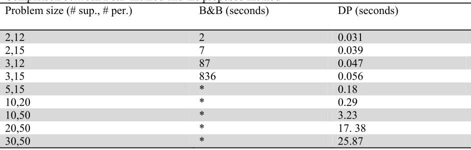
The minimum of these three costs, i.e. 375, will be the value of the last row (“Min” row) of Table 6, which shows that the optimal ordering policy would be as follows: placing an order on supplier 2 to satisfy demands of periods 2 and 3, and placing an order on supplier 1 to satisfy demand of the first period. Similarly, for the fourth column, the minimum cost of 455 is the optimal ordering policy which suggests placing an order on supplier 1 in period 1 to satisfy the demand of this period, and placing an order on supplier 2 in period 2 to satisfy demands of periods 2 through 4. In Table 7, we have compared our proposed dynamic programming method with the branch and bound (B&B) method, which also yields the exact solution, in terms of CPU time (seconds). The first column of Table 7 is the problem size (no. of suppliers, no. of periods). Column 2 is the solution time of the B&B method, and column 3 is the solution time of proposed dynamic programming method. As it can be seen, for the small problem sizes, our method is considerably superior to the B&B method, and for larger problem sizes, while our method has reached the optimal solution in relatively small amount of time, the B&B method has failed to reach to any solution.
Table 7
Comparison between B&B method and the proposed method
Problem size (# sup., # per.) B&B (seconds) DP (seconds)
2,12 2 0.031
2,15 7 0.039
3,12 87 0.047
3,15 836 0.056
5,15 * 0.18
10,20 * 0.29
10,50 * 3.23
20,50 * 17. 38
30,50 * 25.87
5. Conclusion and future research directions
We have presented the supplier selection and lot-sizing problem in which a single product with deterministic demand is ordered from different suppliers for different time periods. Demand of the product is not constant and varies in different time periods. For the sake of simplicity, we ignored restrictions imposed on the warehouse storing space and production capacities of suppliers, and model the problem as a mixed integer linear program (MILP). The main contribution of this paper is the proposed solution method to obtain the optimal solution. Using a recursive relation, we have developed a dynamic programming solution methodology which reduces the search space to obtain
the optimal solution from UT to T*(T+1)/2*U. This way, by reducing the search space from
polynomial time to linear time, efforts to obtain the optimal solution, especially for large scale and practical problems, have considerably been decreased, such that in some large-scale cases the optimal solution can be reached in a reasonable amount of time. Finally, we have illustrated the solution algorithm both in the step-by-step and tabular forms, and presented a numerical example to show the high efficiency of the proposed method. As a future research direction, the proposed relation and solution algorithm can further be developed to handle the multi-product cases.
References
Aissaoui, N., Haouari, M., & Hassini, E. (2007). Supplier selection and order lot sizing modeling: A
review, Computers & operations research, 34, 3516–3540.
Aryanezhad, M.B.G. (1992). An algorithm based on a new sufficient condition of optimality in
Basnet, C., & Leung, J.M.Y. (2005). Inventory lot-sizing with supplier selection, Computers and Operations Research, 32, 1–14.
Brahimi, N., Dauzere-Peres, S., Najid N.M. & Najid, A. (2006). Single item lot sizing problems,
European Journal of Operational Research, 168, 1-16.
Cattrysse, D., Maes, J., & Van Wassenhove, L.N. (1990). Set partitioning and column generation
heuristics for capacitated dynamic lot-sizing, European Journal of Operational Research, 46,
38–48.
Current, J., & Weber, C. (1994). Application of facility location modelling constructs to vendor
selection problems, European Journal of Operational Research, 76, 387–92.
Dai, T., & Qi, X. (2007). An acquisition policy for a multi-supplier system with a finite-time horizon,
Computers & Operations Research, 34, 2758 – 2773.
Evans, J.R. (1985). An efficient implementation of the Wagner–Whitin algorithm for dynamic lot
sizing, Journal of Operations Management, 5, 235–239.
Hassini, E. (2008). Order lot sizing with multiple capacitated suppliers offering leadtime-dependent
capacity reservation and unit price discounts, Production Planning & Control, 19, 142–149.
Heady, R.B., & Zhu Z. (1994). An improved implementation of the Wagner–Whitin algorithm,
Production and Operations Management, 3, 55–63.
Liao, Z., & Rittscher, J. (2007). Integration of supplier selection, procurement lot sizing and carrier
selection under dynamic demand conditions, Int. J. Production Economics, 107, 502–510.
Rezaei, J., & Davoodi M. (2006). Genetic algorithm for inventory lot-sizing with supplier selection
under fuzzy demand and costs, Advances in Applied Artificial Intelligence, 4031, 1100–1110.
Rezaei, J., & Davoodi, M. (2008). A deterministic multi-item inventory model with supplier
selection and imperfect quality, Applied Mathematical Modelling, 32, 2106–2116.
Rosenblatt, M. J., Herer, Y. T., & Hefter, I. (1998). An acquisition policy for a single item
multi-supplier system, Management Science, 44, 96–100.
Sadjadi, S. J., Aryanezhad, M.B.G., & Sadeghi, H.A. (2009). An Improved WAGNER-WHITIN
Algorithm, International Journal of Industrial Engineering & Production Research, 20,
117-123.
Tempelmeier, H. (2002). A simple heuristic for dynamic order sizing and supplier selection with
time-varying data, Production and Operations Management, 11, 499–515.
Ustun, O., & Demirtas, E. A. (2008a). An integrated multi-objective decision-making process for
multi-period lot-sizing with supplier selection, Omega, 36, 509 – 521.
Ustun, O., & Demirtas, E. A. (2008b). Multi-period lot-sizing with supplier selection using
achievement scalarizing functions, Computers & Industrial Engineering, 54, 918–931
Wagner, H. M., & Whitin, T.M. (1958). Dynamic version of the eonomic lot-size model,
Management Science, 5, 89–96.
Wolsey, L. A. (1995). Progress with single-item lot-sizing, European Journal of Operational