METHODOLOGY
Land-based crop phenotyping by image
analysis: consistent canopy characterization
from inconsistent field illumination
Joshua Chopin
*, Pankaj Kumar and Stanley J. Miklavcic
Abstract
Background: One of the main challenges associated with image-based field phenotyping is the variability of illumination. During a single day’s imaging session, or between different sessions on different days, the sun moves in and out of cloud cover and has varying intensity. How is one to know from consecutive images alone if a plant has become darker over time, or if the weather conditions have simply changed from clear to overcast? This is a signifi-cant problem to address as colour is an important phenotypic trait that can be measured automatically from images. Results: In this work we use an industry standard colour checker to balance the colour in images within and across every day of a field trial conducted over four months in 2016. By ensuring that the colour checker is present in every image we are afforded a ‘ground truth’ to correct for varying illumination conditions across images. We employ a least squares approach to fit a quadratic model for correcting RGB values of an image in such a way that the observed values of the colour checker tiles align with their true values after the transformation.
Conclusions: The proposed method is successful in reducing the error between observed and reference colour chart values in all images. Furthermore, the standard deviation of mean canopy colour across multiple days is reduced significantly after colour correction is applied. Finally, we use a number of examples to demonstrate the usefulness of accurate colour measurements in recording phenotypic traits and analysing variation among varieties and treatments. Keywords: Wheat, Colour, Phenomics, NDVI
© The Author(s) 2018. This article is distributed under the terms of the Creative Commons Attribution 4.0 International License (http://creat iveco mmons .org/licen ses/by/4.0/), which permits unrestricted use, distribution, and reproduction in any medium, provided you give appropriate credit to the original author(s) and the source, provide a link to the Creative Commons license, and indicate if changes were made. The Creative Commons Public Domain Dedication waiver (http://creat iveco mmons .org/ publi cdoma in/zero/1.0/) applies to the data made available in this article, unless otherwise stated.
Background
The century-old [1] endeavour to understand complex genotype × environment (G × E) interactions and their effect on plant phenotype has triggered a series of break-throughs in the field of plant phenotyping. Manual meth-ods for recording phenotypic traits gradually evolved [2] to semi-manual and automatic methods, through the use of electronic hand-held devices and imaging equip-ment. Automated phenotyping through image capture and analysis was first achieved with state of the art robot-ics and imaging sensors in controlled environments [3–
7]. More recently, in order to further understand G × E interactions, the ‘environment’ side of the equation has
increased in accuracy thanks to phenotypic analysis in the field [8–11].
The range of phenotyping that can occur in the field is vast. Hardware solutions that have been proposed range from aerial imaging [12, 13], large and expensive purpose-built systems [14, 15], small and expensive purpose built systems [16–18] to small and inexpen-sive systems [19, 20]. While each approach possesses distinct advantages and disadvantages, the increase in throughput and volume of high resolution RGB (Red, Green and Blue channel) data offered by imaging of field trials comes at a cost: new methodologies are required to overcome new challenges. In this article the challenge of accurately recording plant colour under varying illumination conditions in the field is con-sidered. In essence, the critical question is how is one to know from consecutive images alone if a plant has
Open Access
*Correspondence: [email protected]
become darker over time, or if the weather conditions have simply changed from clear to overcast? Despite colour being reported as an important plant pheno-typic trait [2, 21, 22] indicative of plant health, an early indicator of a state of stress or disease, and related to plant chlorophyll [23, 24] and nitrogen content [25], it has been largely neglected in the literature until recently [14, 15, 26].
Existing approaches to compensate for variations in illumination can be classified as hardware or soft-ware solutions. Utilising the camera’s hardsoft-ware, a com-mon approach is to simply use the ‘automatic-exposure’ mode on digital cameras [14, 15, 27], which makes use of the camera’s in-built metering system to automati-cally decide on an appropriate shutter speed and aper-ture. This approach comes with a number of drawbacks such as spherical aberration [28] and a lack of consist-ency in recording colour. From a theoretical standpoint the computer vision community has proposed many post-processing techniques to determine the illuminant in an image, which they call the colour constancy prob-lem. For example, Finlayson et al. [29] used histogram equalization to provide illumination invariance across devices and before that calculated individual likelihoods that each possible scene illuminant was illuminating the test image [30]. Forsyth [31] estimated the illuminant in images using surface reflection functions and D’Zmura et al. [32] showed that in an arbitrary scene the chromac-ity of reflected light from at least four surfaces is required to estimate illumination.
In the case of field-based phenotyping, most image analysis approaches taken to the illumination chal-lenge focus on accurately determining canopy cover-age or other traits, rather than correcting the canopy colour itself. For example, in [33] the authors propose a method for image segmentation that is invariant to illu-mination. However, the segmented plant still contains the illuminated pixels. In [34] the authors train two sepa-rate support vector machines, for high and low lumi-nance, then propose an approach to classify every image as one of those two, before applying the respective SVM for segmentation. Both of these examples are useful for approximating coverage, yet provide misleading colour information. In a study closely related to the present work, Grieder et al. [35] made use of a colour checker for standardizing colour images over a day but only used a linear transformation to correct the colour values. We will show that for images in the field a quadratic model is more accurate. Furthermore, as that study was focussed on assessing canopy coverage of plots, an investigation into the accuracy of colour measurements over time and how robust they are to varying illumination conditions was not within the scope of their article.
In this paper we propose the use of an X-rite Colour Checker chart [36] and a quadratic model for correcting the colour of plant images taken in the field. Two stand-ard digital cameras and a colour chart are mounted on an inexpensive, land-based vehicle in order to capture a time series of high resolution images of individual plots of a wheat field over a period of four months. The details of this field trial and the construction of the vehicle are explained in the Methods section. An image processing pipeline for analysing the images, comprised of pre-pro-cessing and segmentation stages, is also provided in this section. A quadratic model is then used to ascertain the relationship between observed and reference colour chart values for every image and the appropriate transforma-tion is applied to each of them. In the Results sectransforma-tion we demonstrate the effectiveness of the quadratic model and produce evidence of its robustness over multiple days. Finally, we provide examples illustrating the application of accurate colour measurement by studying variations across varieties and treatments, as well as predicting the normalized difference vegetation index of plants using mean canopy colour.
Methods
The field trial was conducted at Mallala (− 34.457062, 138.481487), South Australia, in a randomized complete block design with a total of 60 plots consisting of ten spring wheat (Triticum aestivum L.) varieties and six rep-licates for each. To mitigate the effects of border rows, an additional plot (not included in the analysis) was planted at the beginning and end of each row of plots. Plots were 1.2 m wide and 4 m long with a gap of approximately 1 m between columns and rows. Half of the replicates were treated with nitrogen at a standard rate of 80 kg nitrogen, 40 kg phosphorus and 40 kg potassium per hectare and the other half received no treatment. The macronutrients nitrogen, phosphorus and potassium were first applied on 12 August 2016 and imaging of the plots took place between August 23 and November 18 of the same year. A detailed report on the outcome of this field experiment is the subject of a separate communication.
Images were acquired using a stereo pair of Canon EOS 60D digital cameras, placed approximately 20 cm apart and 2 m above ground level. Manual focus was used dur-ing all imagdur-ing sessions with cameras focused at 2 and 1.5 m during early and late plant growth stages, respec-tively. Camera settings were as follows; focal length 18 mm, aperture f/9.0, ISO—automatic and exposure time 1/500 s. Cameras were temporally synchronized to capture images within 1 ms of each other.
Image processing
All image processing and analysis steps were conducted in MATLAB 2017a. A flowchart outlining each step of the image analysis pipeline is shown in Fig. 2. While this section provides an overview of each image process-ing task associated with analysprocess-ing images from the field, a more detailed explanation can be found in Additional file 1.
Before applying the colour correction technique to images from the field two important pre-processing steps were taken. Both of these steps are necessary due to challenges arising from field conditions. The two pre-processing steps are detecting the region of inter-est (ROI), the image region containing plant pixels, and extracting the colour checker. To provide consistency in the analysis of images of all plant varieties and through-out the season, with the added benefit of avoiding spuri-ous contributions from weeds present in the images but lying outside the ROI, the ROI was chosen to be all pixels inside the parallel rails of the phenotyping vehicle. From an image processing perspective this involves detecting the two rails, using a Hough transform [37], and creating a mask the same size as the original image which, after the application of a Hadamard product [38], removes the background regions outside of the ROI perimeter (Addi-tional file 1: Fig. S1). The colour chart is extracted using a template matching algorithm which iteratively searches the image for regions which resemble a pre-saved generic image of a colour checker.
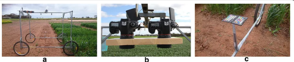
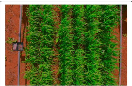
After image pre-processing the next step is segmenta-tion. Plant pixels in all images were segmented from the background using support vector machines (SVM) [39] which were trained on the output of k-means cluster-ing [40]. SVM is a supervised machine learning tech-nique which, for a set of data with two classes, attempts to find the best hyperplane that separates the two data classes. Using k-means clustering, each training image is segmented into 20 clusters with minimal intra-class vari-ance, then each cluster is given a label as green plant or background. The centre of each cluster, or mean colour, is then used as an individual training data point for the SVM (Additional file 1: Fig. S2). As this process takes Fig. 1 Imaging wagon. a The ground based vehicle for imaging in the field. b Two stereo cameras are placed in the centre of the top section, with a third camera at an oblique view not used in this experiment. c An x-rite colour checker is also placed on the side of the vehicle, visible by the camera on the same side
far less time than manually segmenting entire images, it allows more total images to be used for training, captur-ing more variation across plots and over time.
Colour correction
The goal of colour correction is to transform the pixel values in an image in such a way that the observed ues of the colour checker tiles will match their true val-ues after the transformation. This requires constructing a model using the observed values from the colour checker in an image, which can take as input a new colour triplet and output its corrected values. In this article we have chosen to conduct the colour correction stage in the CIEL*a*b* 1976 colour space, abbreviated as L*a*b* here-inafter. The L*a*b* space was chosen as it was designed to be a device-independent space. In addition, through experimentation and following a review of the literature, the L*a*b* space was found to perform better generally than the RGB space for colour correction [41]. While the L*a*b* space was determined to be the most useful for performing colour correction, all results have been con-verted back to RGB values for illustrative purposes, since the RGB space mimics human vision and each channel contains values in the same range of [0, 255]. Conversion between RGB and L*a*b* values is carried out using the standard formulae [42].
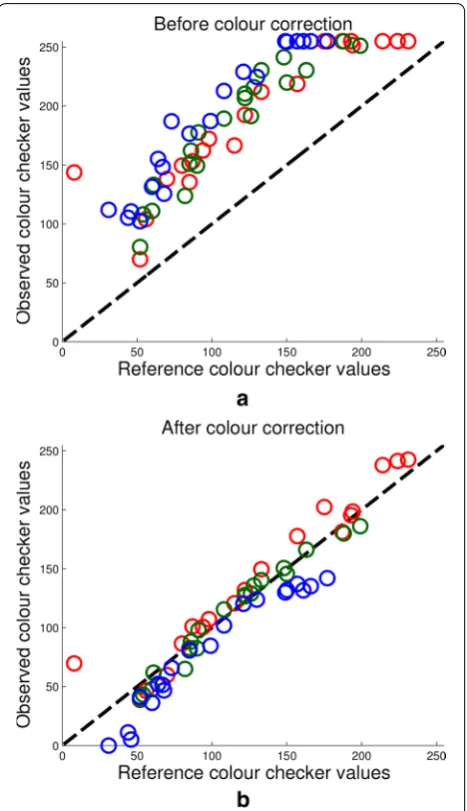
Figure 3a shows the relationship between true and observed RGB values of the 24 colour checker tiles for a typical image. As the relationship does not appear to be linear, a quadratic model was chosen to fit the data. As an aside, this model was used to fit all 24 tiles as well as a number of subsets of tiles, in order to determine whether the range of colours provided by the colour checker was appropriate. We found that using all tiles provided the best results and most versatile model. The quadratic model makes use of all three channels and their squares when predicting colour values. For example, the formula-tion for the L∗ channel is as follows,
where Li , ai and bi refer to the observed L∗ , a∗ and b∗
values of the i-th colour checker tile, α refers to the
fit-ting coefficients and Lˆi refer to the L∗ reference values of
the i-th tile. The same methodology is used with β and γ
(1)
coefficient values for the a∗ and b∗ channels, respectively.
Finally, the least squares method is used to determine the values of α , β and γ . Applying the model to the observed
colour checker values shown in Fig. 3a, after correction yields the results shown in Fig. 3b.
Results and discussion
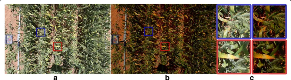
An example of a colour corrected image of a field plot is shown in Fig. 4. The magnified image regions illustrate the increased contrast between healthy and senesced plant regions in later stages of plant life. We demon-strate the usefulness of colour correction by first illustrat-ing the increase in accuracy and consistency it provides when measuring mean canopy colour in the field. Fixing
Fig. 3 Colour correction. a Reference colour checker values vs observed colour checker values before colour correction takes place.
camera settings and applying colour correction, rather than relying on camera automatic-exposure settings, is preferential for a number of practical reasons which will be explained in this section. However, to prove this point in a quantitative manner, the reproduction error of colours for each approach is calculated. Once it is established that colour corrected images are more useful than uncorrected images we show how they can be used in typical phenotypic analyses. This includes outlining key differences in time series data of mean canopy col-our for wheat plots of different varieties under different treatment conditions. Furthermore, we show that col-our corrected images can be used to find relationships between the RGB values of plot canopies and their manu-ally measured normalized difference vegetation index (NDVI) values.
Quantifying the importance of colour correction
While most literature concerning image-based pheno-typing in the field do not perform colour correction at all, the few that do use a simple linear scaling of pixel val-ues [35]. However, the observed pixel values in images compared to their true values, as shown in Fig. 3, appear to follow a quadratic rather than linear relationship. To compare how well the data is fit by linear and quadratic models, we compare the approach outlined by Grieder et al. with the method presented here. The dashed and solid lines in Fig. 5a, b show the R2 values of linear and
quadratic fits of the observed colour values, respectively. The values on the horizontal axis represent the 60 plots of wheat used in the field trial, ordered in order of increas-ing illumination. That is, the first data point represents the plot with the largest difference between observed and reference colour checker values. The mean square error (MSE) can be seen on the left side horizontal axis and is illustrated by the dashed black line.
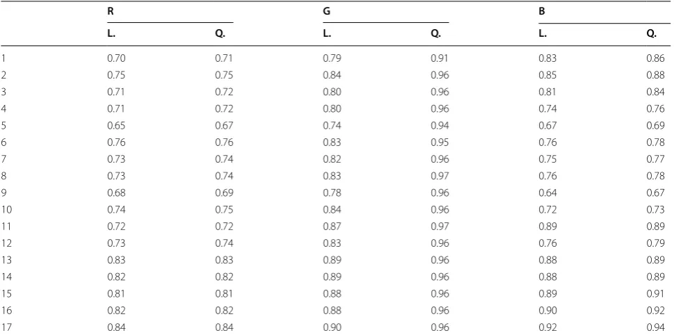
Figure 5a, b represent two different days during the experiment, therefore changes in illumination with time will also be different and as such the order of plots is not maintained between figures. The purpose of this choice for visualization is two-fold. First, one can see that on these 2 days the quadratic model always provided a more accurate fit of the data. Furthermore, while the improve-ment between a linear and quadratic fit is insignificant in the red and blue channels, it is substantial in the green channel. As the defining characteristic of plant pixels is their green intensity, this is the most important channel to correct. Table 1 shows the mean R2 values for fitting
a quadratic or linear model to the red, green and blue channels over the 17 imaging sessions. While the average difference in R2 value between a linear and quadratic fit
in the red and blue channels is 0.05 and 0.02 respectively, it is a substantially higher 0.12 in the green channel.
The second reason for ordering the data in order of illumination is to highlight how the illumination con-ditions affect the goodness of fit for these models, and subsequently the accuracy of the final colour correction. The two examples in Fig. 5a, b show that there is a clear inverse relationship between the degree of illumination and how well the two methods were able to fit the colour data in the red and blue channels. The green channel has not only been fit with larger R2 values overall, but appears
to also be less affected by illumination conditions when fit with a quadratic model.
Figure 6 shows the mean and standard deviation of error between observed and reference colour checker val-ues, over all 16 imaging sessions, before and after the col-our correction process, using the quadratic model. The error, E, which is the average Euclidean distance between the two colour triplets or mean square error (MSE), is calculated according to Eq. 2, where R, G and B denote the red, green and blue colour channels respectively,
Ri denote the reference and observed red values of the ith
tile, respectively, and similarly for G, green, and B, blue. The amount of error after colour correction is approxi-mately four times lower than before it was applied. Fur-thermore, there is more variation across imaging sessions when colour correction is not applied, as error rates
increase and decrease over time with no predictable pat-tern. This is due to the different illumination conditions and the effect they have on colour correction. Therefore, another meaningful analysis is to investigate how well the colour correction process is able to maintain a consistent measure of colour for each plot across multiple days. Fig. 5 Quadratic fits over a day with a constant change in illumination and b step-changes in illumination. Graphs displaying the R2 value of a linear
Table 1 R2 values for linear (L.) and quadratic (Q.) fits of the red (R), green (G) and blue (B) data for 17 imaging sessions (rows), averaged over the 60 plots each time (columns)
R G B
L. Q. L. Q. L. Q.
1 0.70 0.71 0.79 0.91 0.83 0.86
2 0.75 0.75 0.84 0.96 0.85 0.88
3 0.71 0.72 0.80 0.96 0.81 0.84
4 0.71 0.72 0.80 0.96 0.74 0.76
5 0.65 0.67 0.74 0.94 0.67 0.69
6 0.76 0.76 0.83 0.95 0.76 0.78
7 0.73 0.74 0.82 0.96 0.75 0.77
8 0.73 0.74 0.83 0.97 0.76 0.78
9 0.68 0.69 0.78 0.96 0.64 0.67
10 0.74 0.75 0.84 0.96 0.72 0.73
11 0.72 0.72 0.87 0.97 0.89 0.89
12 0.73 0.74 0.83 0.96 0.76 0.79
13 0.83 0.83 0.89 0.96 0.88 0.89
14 0.82 0.82 0.89 0.96 0.88 0.89
15 0.81 0.81 0.88 0.96 0.89 0.91
16 0.82 0.82 0.88 0.96 0.90 0.92
17 0.84 0.84 0.90 0.96 0.92 0.94
0 2 4 6 8 10 12 14 16 18
1 2 3 4 5 6 7 8 9 10 11
Time
Mean Square Error
Error of observed colour chart tiles
After colour correction Before colour correction
Figure 7 shows mean canopy colour in the red, green and blue channels for a sample wheat plot over all 16 imaging sessions. The purpose of this plot is not to demonstrate the mean intensities themselves but rather to depict the consistency of colour measurements over multiple days with varying levels of illumination. The jagged nature of the dashed lines, colours before correction, implies changes in colour too severe and irregular to be associ-ated with a biological phenomena. Instead, the mean intensities are changing over time primarily due to imag-ing sessions beimag-ing conducted on bright or overcast days. On the other hand, the solid lines, representing colour values after correction, appear much more stable over a long period of time. It is also of note that the steady rise in pixel intensities in the colour corrected data toward the end of the experiment is to be expected, as plants are beginning to senesce and turn yellow, which has higher red intensities than green. Table 2 shows the standard deviation of mean canopy colour over the 16 days for all 60 plots in the trial. In no case did the standard devia-tion of corrected values exceed the standard deviadevia-tion of uncorrected ones, which were 63% higher, on average.
(2)
E = 1
24 24
i=1
(Rˆi−Ri)2+(Gˆi−Gi)2+(Bˆi−Bi)2
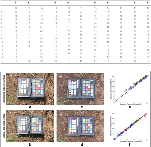
Automatic exposure settings versus colour correction
The automatic exposure mode of standard digital cam-eras uses the camera’s in-built metering systems to automatically choose values for the aperture and shut-ter speed parameshut-ters. However, allowing the maximum amount of light to hit the camera’s sensor by choosing the minimum safe shutter speed which will avoid motion blurring is preferable to letting the camera choose the shutter speed parameter on a per-image basis. Further-more, in repeated experiments with a fixed schematic the depth of field, related to the aperture, should remain consistent.
Besides the artifacts affecting image quality, perform-ing colour correction after imagperform-ing with a fixed exposure outperforms the use of auto-exposure features in terms of colour consistency. Figure 8 presents results of a short experiment comparing the two approaches. Sample images of the colour checker in well-lit field conditions taken with automatic and with manual exposure settings are shown in Fig. 8a, b, respectively. The same object is imaged in simulated overcast conditions, shown in Fig. 8c, d, using automatic and manual exposure settings, respectively. Figure 8e, f are plots showing the differ-ence in colour values after illumination conditions have changed, when using automatic and manual exposure settings, without and with colour correction, respectively. It is clear that using automatic exposure settings has not completely corrected for the change in illumination,
2 4 6 8 10 12 14 16
0 50 100 150 200 250
Mean canopy colour over time
Time
Intensity
Red Green Blue
Red Corrected Green Corrected Blue Corrected
with all colour values having increased. In fact, the mean square error in colour values between the two illumina-tion condiillumina-tions is more than twice as large when using automatic exposure, 4.26, compared to manual exposure settings, 1.57.
Colour corrected images for analysing variation in plant varieties and treatments
In this section we will use a number of colour corrected images to show the variations in canopy colour between different varieties, different treatments and different time periods that can be analysed. Note that Fig. 7 shows
Table 2 Standard deviation of green intensity values over 16 imaging sessions for the 60 plots before (B) and after (A) the application of colour correction
B A B A B A B A
1 19 10 16 13 9 31 15 14 46 13 10
2 16 10 17 14 8 32 15 9 47 19 7
3 13 8 18 12 9 33 15 8 48 16 11
4 13 12 19 15 8 34 17 10 49 20 17
5 14 10 20 14 7 35 14 10 50 15 11
6 12 9 21 11 11 36 14 10 51 16 11
7 14 11 22 11 9 37 14 12 52 11 8
8 12 10 23 13 6 38 18 10 53 15 8
9 16 7 24 16 9 39 18 10 54 17 7
10 16 10 25 17 7 40 17 10 55 14 10
11 14 9 26 14 9 41 15 9 56 14 9
12 15 11 27 13 9 42 15 9 57 21 16
13 16 11 28 14 9 43 17 9 58 19 10
14 15 11 29 15 5 44 15 11 59 14 10
15 17 8 30 18 7 45 13 8 60 14 9
consistently small values in the blue channel, regard-less of inconsistencies in illumination. This is due to plants reflecting larger amounts of red and green light than blue light in general. Due to this fact, hereinafter results will only be presented for the red and green chan-nel, as they capture a large proportion of the variation in
plot colour. Furthermore, a main part of this study will revolve around the two treatments applied to the plots, as a result they will hereinafter be abbreviated as fertilized (F) and non-fertilized (NF).
The first result of this study, shown in Fig. 9, supports the hypothesis formed in the previous section, based on the contents of Fig. 7, that even under inconsistent field con-ditions colour corrected images are consistently able to exhibit the senescence stage of plants. Figure 9a shows that in the early, healthier, stages of plant life the green values of mean canopy colour are found almost exclusively above the red values, by a substantial margin, in fertilized plots. However toward the end of the time series the relationship is inverted and the intensity of red values is much higher. The same phenomenon can be seen in Fig. 9b, except here the separation between red and green values is not as dis-tinct. Note that this is due to red values increasing in the NF plots, rather than green values decreasing, perhaps implying an early onset of decreased plant health.
A range of post-harvest manual measurements were also obtained for the wheat plots grown in this study. The data from these measurements supports the hypothesis that mean plant canopy colour can be useful as a phenotypic trait that is related to other important traits such as yield. For example when averaging over the three replicates of each, the difference in total post-harvest biomass weight between F and NF plots of the same variety is 21.1 g. In the case of Gregory plots, the average difference in biomass between F and NF plots is 122 g. Similarly, the difference in straw weight between all F and NF plots is, on average, 26.5 g. However, for Gregory plots the difference is 82.7 g. Furthermore, Gregory appears to move through devel-opmental stages at a slower rate than the other varieties, remaining on average more than 10 cm shorter than other varieties for most of the experiment.
We can support this manual data using the mean canopy colour information obtained from our colour corrected images. Figure 10 shows the red and green values for mean canopy colour over the length of the experiment for the Gregory, Excalibur, Magenta and Spitfire varieties. Each row shows the red and green values of Gregory plotted against the red and green values of a different variety and the two columns present the data of F and NF plots side by side. The first thing to note is that in all cases, including F and NF, the red values of Gregory are lower than the vari-ety chosen for comparison. This implies that either Greg-ory is senescing significantly less than all other varieties, Fig. 9 Mean intensities of all varieties, fertilized and non-fertilized.
Plot showing the red and green values of ten wheat varieties both
a fertilized and b non-fertilized for 16 imaging sessions. Different colours refer to different varieties, while dashed and solid lines refer to green and red values, respectively
Fig. 10 Corrected colour values for Gregory versus other varieties. Plots showing red and green mean intensities of images of plots of Gregory and Excalibur (a and b), Magenta (c and d) and Spitfire (e and f). Each row represents a different variety comparison with Gregory, while the left and right columns depict results for fertilised and non-fertilised plots, respectively
or, more plausibly, that it is taking longer to reach the stage of senescence, as the post-harvest data would also suggest. Furthermore, Gregory displayed the largest variation in green and red values between N and NF plots during early stages of growth. This can be seen from imaging sessions one to seven especially, where the red and green values in F plots are almost identical yet vary significantly in NF plots. This particular phenotypic trait could share a relationship with the biomass or straw weight which exhibited similar patterns.
Two more examples of variation between varieties and treatments, not involving the Gregory variety, are provided in Fig. 11. Figure 11a, b show that the varieties
Kukri and Spitfire maintain very similar red and green values throughout all time points and both treatments, except for approximately the last third of time points in F plots where Spitfire exhibited much larger red and green values. Which could imply a significantly differ-ent reaction to nitrogen among two varieties which are otherwise very similar. In Fig. 11c, d we can see the converse, where the Mace and Scout varieties differ from each other in a similar pattern for both F and NF plots.
One can also notice that the green values of the non-fertilized Mace variety on day 4 in Fig. 11d show an abnormally high standard deviation. In this case one
of the three images of such plots contained a colour checker that was partially occluded and the algorithm designed for detecting occlusion failed. This particular plot is shown in Fig. 12, where one can see that part of the colour checker is occluded by shadow. Here the colour values of the tiles have been distorted enough to substantially alter the appearance of the image, but not enough to be detected by the threshold used for automatic occlusion detection. While this scenario only occurred a total of five times in more than 1000 test images, it serves as a reminder that clear and consist-ent imaging of the colour checker is paramount to final accuracy.
Finally, we provide an example of how to predict the NDVI of plants based on average canopy colour, in order to further demonstrate the importance and applicabil-ity of colour correcting a time series of plant images. A Trimble GreenSeeker [43] crop sensing system was used to manually measure the plant NDVI for all 60 plots on five select, approximately uniformly spaced, days of the experiment. NDVI has been used to estimate crop yield and is also directly related to other phenotypic traits such as photosynthetic activity and biomass. Equation 3 pro-vides the formula for calculating plant NDVI, where NIR and R denote the near-infrared and red values recorded by the GreenSeeker system, respectively.
This comparison is especially useful as NDVI values are independent of illumination conditions, since the sum (3)
NDVI= NIR−R
NIR+R,
in the denominator of Eq. 3 ensures that plant patches that are more illuminated are scaled down in magnitude. The first 4 days are used as training data, where the aver-age canopy colour and NDVI of each plot are known. Using the mean canopy colour of both corrected and uncorrected images, two quadratic models are fitted to the NDVI data using the same approach outlined in the Methods section. The statistical method is then used to predict the NDVI values from plant images taken on the fifth day. This is essentially the scheme proposed by Khan et al. [44].
Figure 13 shows the reference NDVI values in the hori-zontal axis and the predicted NDVI values in the verti-cal axis, for cases with two different colour spaces used as training data. Figure 13a used values from the HSV colour space to predict NDVI values, while Fig. 13b used data from the RGB, HSV, Lab and Luv colour spaces. In both cases it is clear that the training data consisting of colour corrected images, blue circles, has more accurately predicted NDVI values than the uncorrected images, red and orange circles. To quantify the accuracy of prediction we again utilise the MSE to determine error, which in this case is calculated as
where N is the number of samples (60 in this case) and
NDVIi and NDVIi are the reference and observed NDVI values for the ith plot, respectively. Table 3 shows the results of using different colour channels as training data. The table shows that in all cases the corrected mean canopy colour was more accurate than the uncorrected data in predicting the true NDVI values, sometimes by as much as an order of magnitude. It is worth noting that Fig. 13a, b appear to further suggest a relationship between a plot’s mean canopy colour and fertilization of the plot. A further study could be employed to deter-mine the accuracy in predicting whether or not a plot has been fertilized, based on its mean canopy colour. Prelimi-nary results show that this type of study can also provide insight into the behaviour of different varieties. As pre-viously stated, the variety Gregory showed the slowest development of all varieties and a significant difference in mean canopy colour between fertilised and non-fertilised plots. In the NDVI study, predicted and reference NDVI values both showed that Gregory plots contained the greatest difference in mean NDVI values between ferti-lised and non-fertiferti-lised plots.
(4)
E = 1
N N i=1
NDVIi−NDVIi
2 , Fig. 12 Sample image after inaccurate colour correction. In this
Conclusions
The scope of plant phenotyping has expanded to include image-based analysis of the field. While increased capa-bilities increase the potential for phenomics experi-ments they also require more advanced methods of analysis. In this article we have proposed an approach for ascertaining the important trait of plant canopy col-our in a correct, accurate and robust manner. We have shown that using an industry standard colour checker and a quadratic model for colour correction we are able to establish a consistent assessment of colour condition irresepctive of fluctuating illumination. We have dem-onstrated that by performing accurate colour correction we provide an accurate and robust measure of mean canopy colour, a useful phenotypic trait which may be directly related to plant NDVI, but also provides a method for consistently measuring colour over time and over varying levels of illumination. In future work we shall consider the role that colour correction plays on detecting and quantifying plant sensecence in the field.
Authors’ contributions
JC and PK acquired the image data. All authors assisted in analysing the data and manuscript preparation. All authors read and approved the final manuscript.
Acknowlegements
The authors gratefully acknowledge financial support from the Australian Research Council through its Linkage program, Project Number LP140100347. The authors would also like to acknowledge members of the Phenomics and Bioinformatics Research Centre, Dr. Zhi Lu, Dr. Jinhai Cai, Dr. Zohaib Khan and Dr. Hamid Laga, for valuable discussions, as well as Dr. Stephan Haefele from Rothamsted University for the field trial arrangement and Vahid Rahimi-Eichi for manual NDVI readings.
Competing interests
The authors declare that they have no competing interests.
Availability of data and materials
The datasets analysed during the current study are not publicly available due to their size, but subsets of the data are available from the corresponding author on reasonable request.
Consent for publication Not applicable.
Additional files
Additional file 1. Image processing. Figure S1. Extracting the region of interest. First the rails of the wagon from the original image are detected using a combination of grayscale thresholding, Hough transforms and a number of morphological operations. The image is then ‘clipped’ to con-tain only the region of interest, hence removing the possibility of weeds or the colour checker being detected as foreground. Figure S2. Support Vector Machine. The images are segmented using the pictured support vector machine classifier which was trained on the output of the k-means clustering algorithm. The x and y axes are u and v values, respectively, from the Luv colour space. The gray and purple regions represent the green plant class and background class, respectively. The green and black circles represent training data of green plant pixel values and background pixel values, respectively.
Fig. 13 Predicting GreenSeeker values using mean canopy colour. A quadratic model has been used to predict GreenSeeker values recorded from all 60 plots. The black line represents perfect prediction, where reference values would match predicted values exactly. Light and dark blue circles represent where colour corrected images were used as training data for the prediction model, orange and red circles refer to the uncorrected images. a Using mean canopy colour in the HSV colour space for prediction. b Using mean canopy colour in RGB, Lab, HSV and Luv colour spaces for prediction
Table 3 Mean square error (MSE) values for predicting plant NDVI values using the mean canopy colour of different colour spaces, before and after colour correction (CC)
RGB HSV Lab Luv All
Ethics approval and consent to participate Not applicable.
Funding
Australian Research Council Linkage Program, Project Number LP140100347.
Publisher’s Note
Springer Nature remains neutral with regard to jurisdictional claims in pub-lished maps and institutional affiliations.
Received: 8 November 2017 Accepted: 18 May 2018
References
1. Johannsen W. The genotype conception of heredity. Am Nat. 1911;45(531):129–59.
2. Furbank RT, Tester M. Phenomics-technologies to relieve the phenotyp-ing bottleneck. Trends Plant Sci. 2011;16(12):635–44.
3. Campbell MT, Knecht AC, Berger B, Brien CJ, Wang D, Walia H. Integrating image-based phenomics and association analysis to dissect the genetic architecture of temporal salinity responses in rice. Plant Physiology. 2015;168(4):1476–89.
4. Hartmann A, Czauderna T, Hoffmann R, Stein N, Schreiber F. Htpheno: an image analysis pipeline for high-throughput plant phenotyping. BMC Bioinf. 2011;12(1):148.
5. Pound MP, French AP, Murchie EH, Pridmore TP. Automated recovery of three-dimensional models of plant shoots from multiple color images. Plant Physiol. 2014;166(4):1688–98.
6. Golzarian MR, Frick RA, Rajendran K, Berger B, Roy S, Tester M, Lun DS. Accurate inference of shoot biomass from high-throughput images of cereal plants. Plant Methods. 2011;7(1):2.
7. Cai J, Golzarian MR, Miklavcic SJ. Novel image segmentation based on machine learning and its application to plant analysis. Int J Inf Electron Eng. 2011;1(1):79.
8. Araus JL, Cairns JE. Field high-throughput phenotyping: the new crop breeding frontier. Trends Plant Sci. 2014;19(1):52–61.
9. Montes J, Technow F, Dhillon B, Mauch F, Melchinger A. High-throughput non-destructive biomass determination during early plant development in maize under field conditions. Field Crops Res. 2011;121(2):268–73. 10. Montes JM, Melchinger AE, Reif JC. Novel throughput phenotyping
platforms in plant genetic studies. Trends Plant Sci. 2007;12(10):433–6. 11. White JW, Andrade-Sanchez P, Gore MA, Bronson KF, Coffelt TA,
Conley MM, Feldmann KA, French AN, Heun JT, Hunsaker DJ, et al. Field-based phenomics for plant genetics research. Field Crops Res. 2012;133:101–12.
12. Liebisch F, Kirchgessner N, Schneider D, Walter A, Hund A. Remote, aerial phenotyping of maize traits with a mobile multi-sensor approach. Plant Methods. 2015;11(1):9.
13. Duan T, Zheng B, Guo W, Ninomiya S, Guo Y, Chapman SC. Comparison of ground cover estimates from experiment plots in cotton, sorghum and sugarcane based on images and ortho-mosaics captured by uav. Funct Plant Biol. 2017;44(1):169–83.
14. Sadeghi-Tehran P, Sabermanesh K, Virlet N, Hawkesford MJ. Automated method to determine two critical growth stages of wheat: heading and flowering. Front Plant Sci. 2017;8:252.
15. Virlet N, Sabermanesh K, Sadeghi-Tehran P, Hawkesford MJ. Field scana-lyzer: an automated robotic field phenotyping platform for detailed crop monitoring. Funct Plant Biol. 2017;44(1):143–53.
16. Busemeyer L, Mentrup D, Moller K, Wunder E, Alheit K, Hahn V, Maurer HP, Reif JC, Wurschum T, Muller J, et al. Breedvision—a multi-sensor platform for non-destructive field-based phenotyping in plant breeding. Sensors. 2013;13(3):2830–47.
17. Andrade-Sanchez P. Use of a moving platform for field deployment of plant sensors. In: 2012 Dallas, Texas, July 29-August 1, 2012, 2012; pp 2789–2797. American Society of Agricultural and Biological Engineers 18. Shafiekhani A, Kadam S, Fritschi FB, DeSouza GN. Vinobot and vinoculer:
two robotic platforms for high-throughput field phenotyping. Sensors. 2017;17(1):214.
19. Liu S, Baret F, Allard D, Jin X, Andrieu B, Burger P, Hemmerle M, Comar A. A method to estimate plant density and plant spacing heterogeneity: application to wheat crops. Plant Methods. 2017;13(1):38.
20. White JW, Conley MM. A flexible, low-cost cart for proximal sensing. Crop Sci. 2013;53(4):1646–9.
21. Rahaman MM, Chen D, Gillani Z, Klukas C, Chen M. Advanced pheno-typing and phenotype data analysis for the study of plant growth and development. Front Plant Sci. 2015;6:619.
22. Chen D, Neumann K, Friedel S, Kilian B, Chen M, Altmann T, Klukas C. Dissecting the phenotypic components of crop plant growth and drought responses based on high-throughput image analysis. Plant Cell. 2014;26(12):4636–55.
23. Liang Y, Urano D, Liao K-L, Hedrick TL, Gao Y, Jones AM. A nondestructive method to estimate the chlorophyll content of arabidopsis seedlings. Plant Methods. 2017;13(1):26.
24. Riccardi M, Mele G, Pulvento C, Lavini A, dAndria R, Jacobsen S-E. Non-destructive evaluation of chlorophyll content in quinoa and amaranth leaves by simple and multiple regression analysis of rgb image compo-nents. Photosynth Res. 2014;120(30):263–72.
25. Wang Y, Wang D, Shi P, Omasa K. Estimating rice chlorophyll content and leaf nitrogen concentration with a digital still color camera under natural light. Plant Methods. 2014;10(1):36.
26. Kumar P, Miklavcic SJ. Analytical study of colour spaces for plant pixel detection. J Imaging. 2018;4(2):42.
27. Casadesus J, Kaya Y, Bort J, Nachit M, Araus J, Amor S, Ferrazzano G, Maal-ouf F, Maccaferri M, Martos V, et al. Using vegetation indices derived from conventional digital cameras as selection criteria for wheat breeding in water-limited environments. Ann Appl Biol. 2007;150(2):227–36. 28. Stevens M, Paraga CA, Cuthill IC, Partridge JC, Troscianko TS. Using
digital photography to study animal coloration. Biol J Linn Soc. 2007;90(2):211–37.
29. Finlayson G, Hordley S, Schaefer G, Tian GY. Illuminant and device invariant colour using histogram equalisation. Pattern Recognit. 2005;38(2):179–90. 30. Finlayson GD, Hordley SD, Hubel PM. Colour by correlation: a simple,
unify-ing approach to colour constancy. In: The proceedunify-ings of the seventh IEEE international conference on computer vision; 1999, vol. 2, IEEE, pp 835–842. 31. Forsyth DA. A novel algorithm for color constancy. Int J Comput Vis.
1990;5(1):5–35.
32. D’Zmura M, Iverson G, Singer B. Probabilistic color constancy. In: Luce RD, D’Zmura M, Hoffman DD, Iverson G, Romney K, editors. Geometric rep-resentations of perceptual phenomena. Mahwah, NJ: Lawrence Erlbaum Associates; 1995. p. 187–202.
33. Guo W, Rage UK, Ninomiya S. Illumination invariant segmentation of vegetation for time series wheat images based on decision tree model. Comput Electron Agric. 2013;96:58–66.
34. Yu K, Kirchgessner N, Grieder C, Walter A, Hund A. An image analysis pipeline for automated classification of imaging light conditions and for quantification of wheat canopy cover time series in field phenotyping. Plant Methods. 2017;13(1):15.
35. Grieder C, Hund A, Walter A. Image based phenotyping during winter: a powerful tool to assess wheat genetic variation in growth response to temperature. Funct Plant Biol. 2015;42(4):387–96.
36. X-rite ColorChecker Classic. http://xrite photo .com/color check er-class ic. Accessed October 2017
37. Illingworth J, Kittler J. A survey of the hough transform. Comput Vis Gr Image Process. 1988;44(1):87–116.
38. Horn RA. The hadamard product. Proc Symp Appl Math. 1990;40:87–169. 39. Hearst MA, Dumais ST, Osuna E, Platt J, Scholkopf B. Support vector
machines. IEEE Intell Syst Appl. 1998;13(4):18–28.
40. Hartigan JA, Wong MA. Algorithm as 136: a k-means clustering algorithm. J R Stat Soc Ser C (Appl Stat). 1979;28(1):100–8.
41. Mantiuk R, Mantiuk R, Tomaszewska A, Heidrich W. Color correction for tone mapping. Comput Gr Forum. 2009;28:193–202 Wiley Online Library. 42. Busin L, Vandenbroucke N, Macaire L. Color spaces and image
segmenta-tion. Adv Imaging Electron Phys. 2008;151(1):66–162.
43. Trimble GreenSeeker handheld crop sensor. http://www.trimb le.com/ Agric ultur e/gs-handh eld.aspx?tab=Produ ct_Overv iew. Accessed Octo-ber 2017