R E S E A R C H
Open Access
Spatial and temporal estimation of air pollutants
in New York City: exposure assignment for use in
a birth outcomes study
Zev Ross
1*, Kazuhiko Ito
2, Sarah Johnson
2, Michelle Yee
2, Grant Pezeshki
2, Jane E Clougherty
3, David Savitz
4and Thomas Matte
2Abstract
Background:Recent epidemiological studies have examined the associations between air pollution and birth outcomes. Regulatory air quality monitors often used in these studies, however, were spatially sparse and unable to capture relevant within-city variation in exposure during pregnancy.
Methods:This study developed two-week average exposure estimates for fine particles (PM2.5) and nitrogen dioxide (NO2) during pregnancy for 274,996 New York City births in 2008–2010. The two-week average exposures were constructed by first developing land use regression (LUR) models of spatial variation in annual average PM2.5 and NO2data from 150 locations in the New York City Community Air Survey and emissions source data near monitors. The annual average concentrations from the spatial models were adjusted to account for city-wide temporal trends using time series derived from regulatory monitors. Models were developed using Year 1 data and validated using Year 2 data. Two-week average exposures were then estimated for three buffers of maternal address and were averaged into the last six weeks, the trimesters, and the entire period of gestation. We characterized temporal variation of exposure estimates, correlation between PM2.5and NO2, and correlation of exposures across trimesters.
Results:The LUR models of average annual concentrations explained a substantial amount of the spatial variation (R2= 0.79 for PM2.5and 0.80 for NO2). In the validation, predictions of Year 2 two-week average concentrations showed strong agreement with measured concentrations (R2= 0.83 for PM2.5and 0.79 for NO2). PM2.5exhibited greater temporal variation than NO2. The relative contribution of temporal vs. spatial variation in the estimated exposures varied by time window. The differing seasonal cycle of these pollutants (bi-annual for PM2.5and annual for NO2) resulted in different patterns of correlations in the estimated exposures across trimesters. The three levels of spatial buffer did not make a substantive difference in estimated exposures.
Conclusions:The combination of spatially resolved monitoring data, LUR models and temporal adjustment using regulatory monitoring data yielded exposure estimates for PM2.5and NO2that performed well in validation tests. The interaction between seasonality of air pollution and exposure intervals during pregnancy needs to be considered in future studies.
Keywords:Air pollution, Birth outcomes, Particulate matter, Nitrogen dioxide, Land use regression, NYCCAS, Temporal adjustment
* Correspondence:[email protected]
1ZevRoss Spatial Analysis, 120 N. Aurora St Suite 3A, Ithaca, NY 14850, USA Full list of author information is available at the end of the article
Background
Large, population-based studies of the relationship be-tween air pollution and adverse birth outcomes such as low birth weight present a challenge from an exposure assessment perspective [1,2]. The simultaneous need to determine exposures in relevant time windows as well as the need to characterize variation in exposure associated with the spatial location of maternal residences requires accurate data on both temporal and spatial patterns in air pollutant levels.
Studies of air pollution and birth outcomes com-monly rely on continuous monitoring data available from regulatory or other ambient monitors [1,3]. Expo-sure assessment, for example, often involves assigning concentrations based on the nearest continuous monitor or based on inverse distance weighting of the regulatory monitoring network [4-8]. Estimates of exposure can easily be derived from these monitors for exposure windows of interest and have the further advantage that the measurements from a regulatory monitoring net-work tend to be collected using consistent methodology and include extensive quality control. Unfortunately, al-though existing regulatory networks can provide data with high temporal resolution (e.g., daily and hourly data), these networks were generally designed to capture trends in overall ambient concentrations for the com-munity and therefore have sparse geographic coverage within urban areas, which can lead to significant expo-sure misclassification in epidemiologic studies. Although there is wide variability by locality and time period, few urban monitoring networks capture pollutant concentra-tions at more than 20 locaconcentra-tions.
In order to improve estimates of the spatial varia-tion in air pollutants, several studies investigating the links between exposure and birth outcomes have used regression or emissions dispersion models that can ac-count for patterns in traffic and land use near mater-nal residences [9-16]. These models may use data from emissions inventories or raw measured concentrations collected in the course of intensive, short-term sampling campaigns and can provide more highly resolved spatial estimates. Dispersion models can also be used to pro-duce temporally resolved estimates of pollutants but re-quire temporally resolved inputs on meteorology and emissions. While daily and hourly data on meteorology is widely available, corresponding detailed data on emis-sions does not generally exist and must be estimated adding significant uncertainty to modeled predictions. Commonly used vehicle emissions software, for example, estimates hourly emissions using a combination of esti-mated vehicle miles traveled and weights that assign emissions based on estimates of the fleet’s vehicle type, vehicle age, hour of the day and speed [17]. The regres-sion models often used to assign air pollution exposure,
known as land use regression (LUR) models, are gener-ally constructed to estimate exposure for a single time window (e.g., an annual or seasonal average). A limited number of studies have attempted to construct higher temporal resolution estimates by adjusting LUR spatial estimates to reflect regional or citywide temporal trends in pollutants (for examples see [9,10,15,18,19]).
The focus on constructing temporally and spatially re-solved estimates of exposure is critical in studies of birth outcomes. These studies are complicated by confoun-ding associated with the seasonal effects of weather and seasonality in births [20,21] as well as the uncertainty as-sociated with which exposure intervals are of most con-cern [22,23]. As such, birth outcomes studies can benefit from a characterization of how exposure buffer distance (spatial) and averaging time (temporal) affect: (1) the relative contribution of temporal vs. spatial variation to the overall variation of exposure estimates; (2) the cor-relation between two important combustion-related pollutants, PM2.5 and NO2; and (3) the correlations
bet-ween estimated exposures across trimesters.
In order to develop spatially and temporally resolved estimates of exposure and investigate the effects of vary-ing spatial buffer sizes and temporal windows, this study takes advantage of unique data resources in New York City (NYC) to assign exposures to fine particulate matter with aerodynamic diameter of 2.5 micrometer or less (PM2.5) and nitrogen dioxide (NO2) in two-week
win-dows to the maternal residences of 274,996 births. Initi-ated in 2007 as part of New York City’s sustainability plan, PlaNYC [24], the New York City Community Air Survey (NYCCAS) has been collecting a suite of combustion-related pollutants since December 2008. With 150 monitors in a 790 square kilometer area, NYCCAS has the most comprehensive geographic co-verage of any urban air monitoring network in the U.S. The high spatial resolution of the NYCCAS pollution measurements, combined with the large population size of the city, provides unique opportunities for epidemio-logical investigations that require geographically and temporally resolved estimates of air pollution exposure. In this paper, we describe the development of spatially and temporally resolved estimates of PM2.5 and NO2
based on a combination of data from NYCCAS and the local regulatory network. We present the model details, the results of a validation, and characteristics of esti-mated exposures.
Methods
Overview of approach for exposure estimation
In estimating the exposures of pregnant mothers in NYC to PM2.5and NO2, we used two sources of air
the spatial estimates to match gestational exposure inter-vals (e.g., trimesters). The first year of NYCCAS moni-toring was used in LUR models along with geographic data on emissions and land use to generate a spatial sur-face. This spatial surface allowed us to estimate an an-nual average pollutant value at any location in New York City. Two-week average concentrations that correspond to time windows within gestational periods were then computed by temporally adjusting the annual average (spatial) concentrations using a city-wide time series computed from continuous regulatory monitors (for examples of other studies using this approach see [9,10,15]). Combining the two sources of data allowed us to capture both spatial and temporal variation in air pol-lution. In this approach, the relative differences in pollu-tant concentrations between different spatial locations remain the same but absolute concentrations at all lo-cations rise and fall together as city-wide pollutant con-centrations are proportionally modified by temporal variation in city-wide weather conditions.
Data
New York City community air survey data and land use variables
Details on the monitoring network and data collec-tion are described elsewhere [25]. Briefly, as part of NYCCAS, two-week average concentrations of several pollutants at street-level (10–12 feet off the ground) were collected in each of the four seasons at 150 loca-tions in New York City for the period December, 2008 through December, 2010. Logistical considerations pre-cluded monitoring at all 150 sites at the same time. Instead, each of the four seasons was divided into six two-week periods (“sessions”) and 25 monitoring units, randomly assigned, operated in any given two week per-iod (a total of 24 two-week sessions per year). The period of December 2008-December 2009 is referred to here as “Year 1” and was used to develop the spatial models while December 2009-December 2010 (“Year 2”) was used for validation. Annual averages were computed using the four seasonal two-week averages after account-ing for temporal variation usaccount-ing the approach outlined in [18,26] and described in Additional file 1. A wide range of traffic and land use-related variables were de-rived for 15 levels of circular buffer regions (50-1000 m) around NYCCAS monitoring sites using geographic in-formation systems (GIS). These variables included traffic density, truck traffic volume, emissions of residual oil for building heating, tree/grass coverage and others. The full list of variables included is described elsewhere [25,27].
PM2.5and NO2data from regulatory monitors
Raw data from the US Environmental Protection Agency’s (EPA) Air Quality System were retrieved for all hours and
all days from January 1, 2007 to March 31, 2011 for the five boroughs of New York City and neighboring counties in both New York and New Jersey. Hourly records of PM2.5and NO2were averaged into daily values. Daily
av-erages with fewer than 18 valid hourly values were ex-cluded. We limited the data to daily and hourly records without laboratory-related qualifiers or local event quali-fiers (e.g., “Construction/Demolition”, “Unique Traffic Disruption”). We retained data with qualifiers associated with regional events that would likely affect the entire city (e.g.,“Wildfire-U.S.”,“Stratospheric Ozone Intrusion”).
New York City birth data
Birth date, gestational age at delivery (used to generate esti-mated conception date) and the geographic coordinates for maternal residences for all births in New York City 2008– 2010 were obtained from the Bureau of Vital Statistics, New York City Department of Health and Mental Hygiene. The database initially included a total of approximately 380,000 births and 160,000 unique residential locations. After restricting the data to births with 22–42 weeks of gestation, truncating the data to only include births with conception dates between July 31st, 2007 through March 12, 2010 (to avoid the fixed-cohort bias [23]), singleton births, non-smoking mothers, plausible birth weights, and the exclusion of births with congenital malformations, the total number of births was 274,996 at 138,680 unique loca-tions. After the fixed cohort bias adjustment, the distribu-tion of gestadistribu-tional age was consistent across the estimated conception months, with 25th percentile, median, and 75th percentile of 38, 39, and 40 weeks, respectively, but it was negatively skewed (i.e., fewer births with short ges-tation lengths), as expected. The maternal residence represents the residence at the time of the birth. No infor-mation on residential relocation, commuting patterns, or time-activity behaviors shaping individual exposures during pregnancy was available. This study was reviewed and ap-proved by the Institutional Review Board of the New York City Department of Health and Mental Hygiene
Analysis
Computation of spatial estimates (based on data from NYCCAS) through land use regression models
monitoring locations and validation was conducted at the remaining 25 sites. The final regression models were ex-tended to account for residual spatial autocorrelation using kriging with external drift (KED). This approach is analogous to generating predictions using regression, then kriging the residuals and adding the results together ex-cept that all modeling stages are conducted simultan-eously using generalized least squares to ensure correct estimation of the prediction errors [28]. To generate a continuous surface of exposure for visualization and com-putation of block-level and neighborhood level exposure, the KED models were applied to a regular 100 × 100 meter lattice of points covering all of NYC. For presentation purposes, the maps of the 100 × 100 meter lattice were smoothed using inverse distance weighting.
The final KED models were used to assignspatial esti-mates of exposure to PM2.5and NO2to the birth cohort.
Exposure estimates were computed for three different spatial scales: 1) a single estimate at the maternal resi-dence (i.e., a KED estimate at specific XY coordinates); and two estimates that were designed to capture ap-proximate neighborhood exposures including 2) an aver-age of KED estimates at 100 meter grid cells within 300 meters of the mother’s home address (to represent block-level exposure); and 3) an average of KED estimates at 100 meter grid cells within 800 meters (0.5 miles) of the mother’s home address (to approximate the average“ walk-able-distance”neighborhood exposure [29]).
Computation of city-wide temporal trends (based on data from regulatory monitors)
Based on an initial review of the correlations and sea-sonal patterns in the data and discussions with New York State Department of Environmental Conservation staff we limited the raw PM2.5 data to (A) monitors
within the five boroughs of NYC (excluding adjacent counties) and (B) monitors using the Federal Reference Method (FRM parameter code 88101). We limited to FRM monitors because monitors collecting continuous hourly data using the tapered element oscillating mi-crobalance method have a known seasonal bias in the relationship with FRM (with the continuous, hourly mo-nitors underestimating PM2.5 during colder times of
the year) [30]. In total there were 5 NO2and 13 FRM
PM2.5monitors that collected data at some point during
our study period. The monitoring objective category associated with all of these regulatory monitors was
“Population Exposure”, indicating that these monitors were meant to measure urban background concentra-tions relevant to population exposures (as opposed to the impact of a specific pollution source). The monitor-ing sites tend to be located on top of buildmonitor-ings (~20-30 meters above ground) and away from major emissions sources. To avoid spatio-temporal confounding associated
with different monitors operating in different time win-dows, only monitors with at least 75% monitoring com-pleteness inallquarters in 2007 through the first quarter of 2011 were included to cover the 2-week periods that span the exposure estimates for the first conception and last births. Five PM2.5monitors at four different locations
(sites) and two NO2 monitors at two different locations
met our completeness criteria standards.
A city-wide daily average for both PM2.5 and NO2was
computed by averaging daily values across sites. PM2.5
monitoring sites included in the analysis operated on either an every-day schedule (1 site in Queens) or an every-third-day schedule (3 sites, one each in Manhattan, the Bronx and Queens). Although daily concentrations at the Queens site are strongly correlated with the other sites (r = 0.98) concentrations tended to be slightly lower (inter-cept = 0.89, slope = 0.98). To account for this small differ-ence we adjusted the daily values where only the Queens data was available using the linear relationship between the average of all four sites and the value at the Queens site. All NO2 monitors collected data on an every-day
schedule. Similar to PM2.5, days with data from a single
NO2 monitor were adjusted based on the relationship
between that monitor to the average of both monitors (additional detail is provided in Additional file 1). For both pollutants, days with no monitoring data were treated as missing. Days with data from two or three monitors were strongly correlated with averages from all monitors (r > 0.98) and were averaged without adjustment.
Temporal adjustment of spatial estimates–two-week window exposure assignment
Spatial PM2.5 and NO2 estimates for each pregnancy
quarter of 2011). These two-week average exposures during the gestation period are the building blocks of final exposure estimates for the analysis of air pollution and birth outcomes (e.g., trimester averages).
Validation of temporal adjustment approach
As a validation, we predicted the raw two-week concen-trations at the 150 NYCCAS locations in Year 2 (a total of four predictions at each of 150 locations – one for each season) using the temporal adjustment approach discussed above. The predictions were compared to measured concentrations using R2 and the mean abso-lute percentage error. The 600 two-week averages from Year 2 (December 2009-December 2010) were not in-cluded in the spatial or temporal model building and thus provide a good opportunity for validation. We also computed, for comparison, exposure estimates based on a nearest monitor approach whereby we assigned the two-week average measured at the nearest monitor as an estimate of exposure – these results are included in Additional file 1. Additional file 1 also provides detail on the apportionment of spatial vs. temporal variation in the raw Year 2 concentrations.
Characterization of spatial and temporal contributions to exposure estimates for birth outcomes
To assess the impact of differing spatial buffers and tem-poral windows on exposure we estimated PM2.5 and
NO2 concentrations for each birth for several
combi-nations of spatial scale and time window. In particular, spatial exposure estimates were generated at the ma-ternal address as well as within the 300 m and 800 m (0.5 mile) buffers around the maternal address. For com-parability with previous birth outcomes studies, ex-posure estimates at each of these spatial scales were computed for five distinct time windows of interest – the last six weeks of gestation, each of the trimesters and the entire gestation period for each birth [31-36]. Each of the estimates reflects a different level of spatial or temporal smoothing between the extremes of purely spatial (i.e., the regression model estimate at the mater-nal address or buffer region with no temporal adjust-ment) and purely temporal (i.e., estimates based solely on the city-wide time series with no distinction for the location of the maternal residence). To characterize the temporal and spatial contributions to overall variation the estimated exposures were regressed on the citywide average pollution levels. We compared correlation be-tween PM2.5 and NO2in each of these combinations of
buffer distance and averaging periods and we examined the correlation between the estimated exposures. Be-cause our exposure estimation is based on two-week blocks of data, the trimesters are defined as follows in gestation weeks: 1st trimester – 1 through 12; 2nd
trimester – 13 through 26; 3rd trimester – 27+. For those pregnancies that had incomplete (<37 weeks) 2nd and 3rd trimesters (0.3% and 9%, respectively), the tri-mester averages are the average of available two-week block averages.
Results
Spatial estimates
Across all NYCCAS sampling sites in Year 1, annual PM2.5at street level averaged 11.3μg/m3(standard
devi-ation = 2.1 μg/m3). The geographic differences in annual average PM2.5 concentrations were most strongly
associ-ated with nearby truck traffic and with the density of boilers burning residual heating oil (#4 or #6 grade). The final regression model includes the average density of truck traffic within 1600 meters (1 mile), the number of boilers burning residual oil within 1 kilometer, the area of industrial land use within 500 meters, the land area with vegetative cover within 100 meters (an inverse asso-ciation; more vegetative cover was associated with less PM2.5) and overall traffic weighted road density within
100 meters (Table 1). The final spatial, LUR model (before KED) predicted the 25 validation locations, loca-tions that were not part of the original modeling, to within 6% of true values (R2= 0.85). The validation sam-ples were returned to the pool of modeling samsam-ples and the residual spatial autocorrelation was estimated. The model exhibited modest residual spatial autocorrelation. A review of the variogram cloud indicated that three lo-cations had a disproportionate effect on the variogram (these sites had unusually large residuals in comparison to nearby sites) and were excluded from variogram fit-ting. These sites were only removed to fit the variogram, the final regression model and final KED model are based on all 150 locations. The final empirical variogram was fit with an exponential variogram model with a range of 5.5 kilometers. In order to capture the smooth regional patterns exhibited in the residuals, the vario-gram was fit without the first variovario-gram bin (i.e., pairs separated by an average of 0.5 miles were excluded from the variogram fitting). The overall variation explained by the KED model with all samples based on the squared correlation between raw and fitted values is 79%.
Annual NO2averaged 27.2 ppb in Year 1 (standard
de-viation = 8.8 ppb) across NYCCAS sites. Differences in NO2 between locations were most strongly associated
locations, locations that were not part of the original modeling, to within 13% of true values (R2= 0.74). If one validation site with an NO2value of 59 ppb is removed
the R2 increases to 0.80. The validation samples were returned to the pool of modeling samples and the re-sidual spatial autocorrelation was estimated. Similar to PM2.5 the model exhibited modest residual spatial
auto-correlation. Three locations with a disproportionate effect on the variogram were excluded and the final em-pirical variogram was fit with an exponential variogram model with a range of 11.7 kilometers. Similar to the PM2.5 models the three sites were removed only for
variogram fitting and the final regression model and KED model use the full 150 sites. The significance of the nighttime population variable in the KED was dimi-nished (p < 0.15) compared with the multiple regression model but was retained due to the strength of the
variable in the regression. The overall variation explai-ned by the KED model with all samples is 80%.
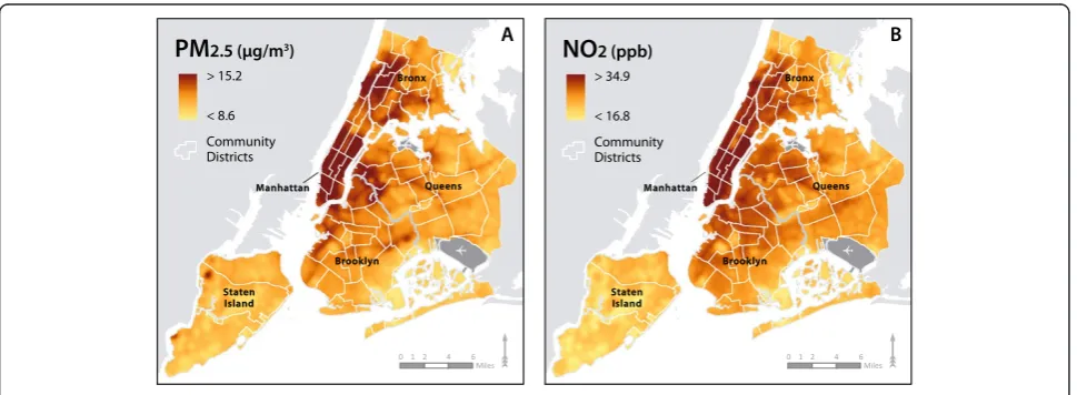
Based on the spatial surfaces of pollutant concen-trations (Figure 1A, B), both PM2.5 and NO2 exhibit
similar geographic patterns with higher concentrations in Manhattan and lower concentrations in Staten Island. Southern areas of the Bronx also exhibit relatively high concentrations for both pollutants while coastal areas have lower concentrations.
The regression-based models were used to generate
“spatial” predictions at maternal residences and on a regular 100 m × 100 m lattice from which we derived the 300 m and 800 m buffer average estimates.
Computation of city-wide temporal trends
Among the regulatory monitoring data there were five PM2.5 FRM monitors at four different NYC locations
Figure 1Map of spatial (KED) estimates for PM2.5and NO2.
Table 1 Land use regression coefficients from the model using kriging with external drift (KED), including the variogram fit
Fine particulate matter model variables Beta Std. error t-value p-value
(Intercept) 10.03 0.28 35.45 <0.01 Exponential variogram model
Industrial land use within 500 m 5.05 1.67 3.02 <0.01 Range (KM) 5.53
Number of boilers burning residual oil within 1 km 0.01 0.00 7.68 <0.01 Partial Sill 0.36
Average density of truck traffic within 1.6 km 0.16 0.06 2.85 0.01 Nugget 0.52
Estimated overall traffic weighted road density within 100 m 0.01 0.00 6.10 <0.01
Land area with vegetative cover within 100 m −57.60 11.43 −5.04 <0.01 Overall R-sq 0.79
Nitrogen dioxide model variables Beta Std. error t-value p-value
(Intercept) 21.11 1.25 16.89 <0.01 Spherical variogram model
Interior square footage of buildings within 1km 0.92 0.10 9.61 <0.01 Range (KM) 18.84
Nighttime population within 1 km 0.00 0.00 1.55 0.12 Partial Sill 3.71
Estimated overall traffic weighted road density within 100 m 0.02 0.00 4.26 <0.01 Nugget 8.15
Location on a bus route (Categorical) 4.94 0.69 7.16 <0.01
(a single site can have multiple monitors) that met our completeness criterion for the data analysis period. In total 0.5% of observations were removed due to EPA database qualifiers. The measurements from the two monitors with complete data at the same monitoring site were highly correlated across all days (r = 0.99) and were averaged within the site. Sites with complete data in-clude a site in northern Manhattan, the Bronx, Queens and Staten Island providing good overall spatial coverage (site details can be found in Additional file 1). All four sites are strongly correlated across the entire time period with bivariate correlation based on daily values ranging from 0.85 to 0.95, providing evidence of a consistent citywide temporal trend. Missing data was imputed (de-tails in Additional file 1) and daily values were averaged. PM2.5 concentrations tend to be elevated both in
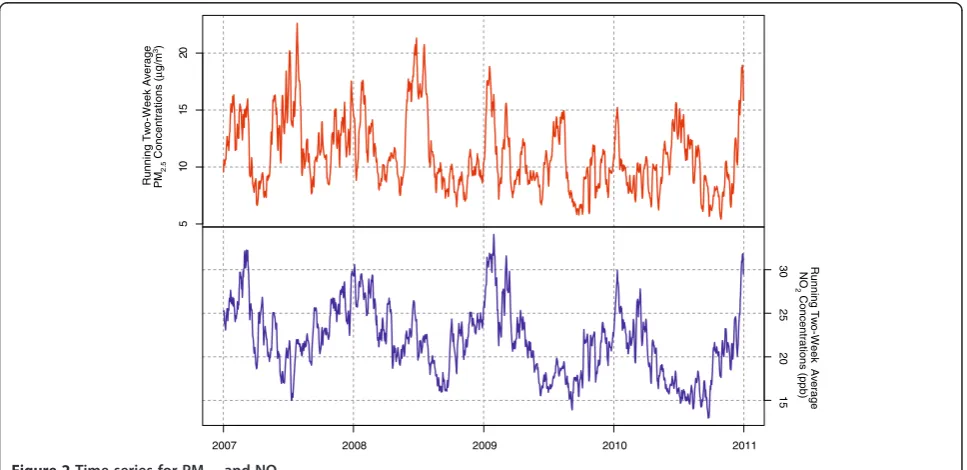
sum-mer and winter (Figure 2). The bi-annual cycle of the PM2.5 temporal pattern reflects alternate contributions
from summer-time chemical constituents (e.g., sulfate) and winter-time chemical constituents (nitrate) to the total PM2.5mass.
There were two monitors with complete NO2 data,
both collecting data every day–one site in Queens and one in the Bronx. No observations were removed due to EPA database qualifiers. Both sites had complete data for all quarters at the 75% threshold except for a single quarter at the site in the Bronx (at this site, the third quarter of 2007 was complete at 68%). We opted to in-clude this site in the computation of the citywide tem-poral trends despite the single quarter slightly below 75% completeness. Missing data was imputed (details in Additional file 1) and daily values were averaged. Daily
values at the two NO2 sites are strongly correlated
across the entire time period (r = 0.88). Concentration peaks occur in the winter (and troughs in the summer) for NO2(Figure 2). The winter peaks likely reflect both
the lower mixing heights (i.e., less atmospheric mixing and ventilation) and increased emissions from oil bur-ning for heating.
Temporal adjustment of spatial estimates
The ratios of two-week (14 day) averages to the yearly average used in the NYCCAS Year 1 modeling for city-wide concentrations ranged from 0.52 to 2.19 for PM2.5
and 0.60 to 1.58 for NO2. These ratios were used to
ad-just the spatial estimates at the maternal residences and generate contiguous two-week averages throughout the gestation period. For validation purposes, the ratios were also applied similarly at NYCCAS monitoring locations to produce two-week predictions corresponding to the two week monitoring periods in Year 2.
Validation of temporal adjustment approach (application to Year 2 NYCCAS data)
In Year 2 measured two-week average PM2.5at NYCCAS
sites ranged from 4.9 to 32.2μg/m3(<1% missing values) and NO2ranged from 7.6 to 58.5 ppb (1% missing values).
Approximately 56% of variation in the raw PM2.5
con-centrations and 18% for NO2is attributable to temporal
variation (details in Additional file 1). The temporal ad-justment method was used to generate predictions of the 600 two-week concentrations of PM2.5 and NO2 from
Year 2. Predictions for both pollutants were strongly correlated with measured concentrations (Figure 3). For
51
0
1
52
0
2007 2008 2009 2010 2011
30
25
20
15
Running T
w
o
-Week A
v
erage
PM
2.5
Concentrations (
µ
g/m
3)
Running T
w
o
-Week
A
v
erage
NO
2 Concentrations (ppb)
PM2.5the R2for predicted vs. actual concentrations (597
non-missing two-week averages) was 0.83 (0.88 if two high concentrations observations are removed) with a mean absolute percentage error of 8%. With the two high con-centration sites removed, the season-specific R2are similar to each other and range between 0.81 and 0.87 (including the two sites decreases the spring R2to 0.73). For NO2the
overall R2(594 non-missing two-week averages) was 0.79 with a mean absolute percentage error of 12%. NO2
pre-dictions were less precise during the winter (R2= 0.72) than for the other three seasons (R2 0.83-0.88) and this pattern is not attributable to a small number of predictions.
Characterization of spatial and temporal components of exposure estimates at maternal residences
For each pollutant, the spatial-only (non-temporally ad-justed) exposure estimates at the three spatial scales (maternal residences and two buffer levels) were highly correlated (r: 0.95 to 0.99 for PM2.5; r: 0.86 to 0.98 for
NO2). The spatial only correlation between the two
pollutants ranged from 0.79 at the maternal address to 0.88 at the 800 m buffer distance.
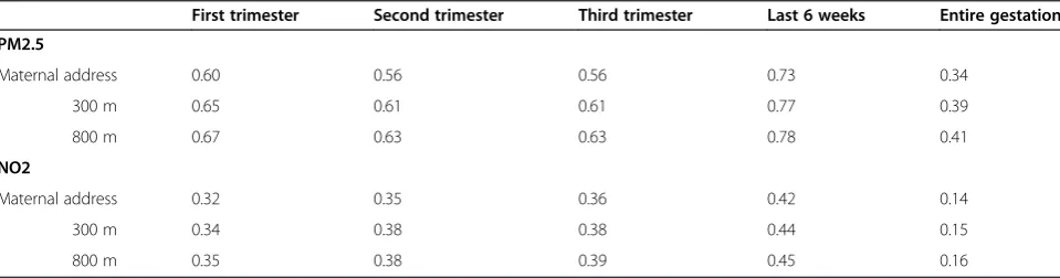
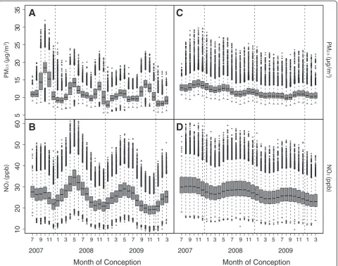
The relative contribution of temporal and spatial vari-ation to the estimated exposures varied between the two pollutants, the exposure interval used and, to a lesser extent, the spatial scale (Table 2). As expected, larger buffer sizes (i.e., more averaging of spatial variation) di-minished the contribution of spatial variation to overall variation, though the magnitude of its impact was not substantial. Likewise, longer averaging time windows resulted in a smaller contribution from temporal var-iation. To illustrate the contrasts, Figure 4 shows box plots of the distribution of the estimated exposures in the birth cohort, sorted by the estimated month of con-ception using two extreme combinations of buffer scale/ exposure averaging time windows from Table 2 (note that the distribution in the first box, July 2007, appears narrow because the cut-off for the adjustment for the fixed cohort bias, July 31st 2007, made all the births in this conception month to be on the same day, restricting time-window variations across births). Figure 4A, B show the distribution of estimated exposures by conception
5 10 15 20 25 30
5
1
01
52
02
53
0
10 20 30 40 50 60 70
10
20
30
40
50
60
70
Figure 3Comparison of measured PM2.5and NO2concentrations vs predictions using the temporal adjustment method.
Table 2 Amount of the overall variation (R2) explained by temporal patterns using varying buffers and averaging exposure interval
First trimester Second trimester Third trimester Last 6 weeks Entire gestation
PM2.5
Maternal address 0.60 0.56 0.56 0.73 0.34
300 m 0.65 0.61 0.61 0.77 0.39
800 m 0.67 0.63 0.63 0.78 0.41
NO2
Maternal address 0.32 0.35 0.36 0.42 0.14
300 m 0.34 0.38 0.38 0.44 0.15
month using the largest buffer distance (800 m) and the shortest exposure averaging window (the last 6 weeks of gestation period), a combination that maximizes the temporal variation. Figure 4C, D show the distribution of exposures using the combination of maternal ad-dress and the longest exposure averaging window (the entire gestation period) a combination that minimizes the temporal variation. On the whole, Figure 4 and the higher R2values for PM2.5in Table 2 indicate that
tem-poral variation contributes more to overall variation for PM2.5than NO2.
The within-pollutant correlations of estimated expo-sures across trimesters are influenced by the pollutant’s temporal (seasonal) variation. Table 3 shows the correla-tions of the estimated exposures across trimesters and the entire gestation period for PM2.5 and NO2 at the
three buffer levels. For PM2.5the estimated exposures in
adjacent trimesters (the 1st and 2nd; the 2nd and 3rd)
are weakly correlated (r = 0.23 to 0.32), but those for the 1st and 3rd trimesters are more strongly correlated (r = 0.73 to 0.76), likely because the 1st and 3rd trimes-ters fall close to peaks/troughs of the bi-annual cycle of PM2.5’s temporal pattern. In contrast to the PM2.5result,
for NO2, the correlations for the estimated exposures in
the adjacent trimesters (r = 0.66 to 0.70) are higher than those between the 1st and 3rd trimesters (r = 0.44 to 0.48), likely because the annual cycle of NO2’s temporal
pattern make adjacent trimesters’ levels more similar. Averaging pollutant concentrations within 3 different buffers around each residence did not substantively change exposure estimates.
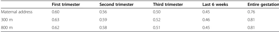
Table 4 summarizes correlations between the esti-mated exposures to PM2.5and NO2for all the
combina-tions of the averaging time windows and spatial buffers. The correlations are the largest when the exposures were averaged for the entire pregnancy periods and the
5
1
01
52
02
53
03
5
10
20
30
40
50
60
1 11
7 9 11 3 5 7 9 11 3 5 7 9
2007 2008 2009
Month of Conception
1 3 7 9 11 3 5 7 9 1 3 5 7 9
2007 2008 2009
Month of Conception
A
B
C
D
1 1 11 11 1 3
smallest for the average of the last 6-weeks of gestation. In other words, the common spatial variation increases the correlation between the two pollutants, and the sea-sonal variations (bi-annual for PM2.5 and annual for
NO2) reduce the correlation.
Discussion
This study describes and validates an approach for as-signing prenatal exposure estimates to PM2.5 and NO2
in a birth outcomes study based on temporally adjusting spatial estimates from a land use regression model. Re-liance on sparse regulatory monitoring networks has significantly constrained the ability of previous studies of birth outcomes to accurately capture geographic vari-ation in prenatal exposure [5,10]. Several recent studies have been able to take advantage of non-regulatory mo-nitoring networks to vastly expand geographic coverage [9,37], but NYCCAS, with 150 monitors in an area of 790 square kilometers, has significantly higher density than previous birth outcomes studies in major urban areas with a very large number of births available for analysis. This monitor density afforded a unique oppor-tunity to capture geographic variation in PM2.5and NO2
in the largest city in the US.
We found that the temporal adjustment approach predicted measured values in the validation well. We further found that the overall variation in PM2.5is more
strongly influenced by temporal variation than NO2.
This likely reflects differences in sources of these pollut-ants. A significant percentage of PM2.5 concentrations
originates from non-local sources (e.g., transported sul-fate) and blankets the city relatively evenly reducing spatial variation [38]. The larger local contribution to NO2 by traffic and oil burning, on the other hand,
re-sults in greater overall spatial variation. The extent of the temporal contribution to the overall exposure var-iation, correlation between the two pollutants and cor-relations across trimesters varied depending on the averaging time window of exposures. The three spatial buffers made only a small difference in the parameters examined. These results are useful in interpreting results from a health effects analysis and in comparing the re-sults from the study using these estimates to previous research.
Implicit in adopting this temporal adjustment ap-proach is the assumption that relative spatial differences in pollutant levels remain constant across the time win-dows relevant to birth outcomes studies (e.g., trimesters) [1]. The high site-level correlation between concentra-tions in different seasons and years of monitoring pro-vides strong evidence for this assumption. For example, the correlation between annual concentrations of PM2.5
and NO2at NYCCAS locations in Year 1 compared with
concentrations at these same locations in Year 2 is 0.93 Table 3 Within-pollutant correlations (Pearson’s r) between different temporal averaging windows and spatial scales
PM2.5 NO2
1st trimester 2nd trimester 3rd trimester 1st trimester 2nd trimester 3rd trimester
Maternal address
2nd Trimester 0.32 - - 0.70 -
-3rd Trimester 0.76 0.32 - 0.48 0.69
-Entire gestation 0.85 0.69 0.86 0.83 0.92 0.84
300-meter buffer
2nd Trimester 0.26 - - 0.69 -
-3rd Trimester 0.74 0.26 - 0.45 0.67
-Entire gestation 0.84 0.66 0.84 0.81 0.92 0.83
800-meter buffer
2nd Trimester 0.24 - - 0.68 -
-3rd Trimester 0.73 0.23 - 0.44 0.66
-Entire gestation 0.84 0.65 0.84 0.81 0.92 0.83
Table 4 Correlations (Pearson’s r) between PM2.5and NO2for varying buffers and averaging exposure interval
First trimester Second trimester Third trimester Last 6 weeks Entire gestation
Maternal address 0.60 0.56 0.50 0.45 0.76
300 m 0.63 0.59 0.52 0.46 0.81
(Pearson’s r) and 0.96, respectively. In addition, site-level correlations between the 8 seasonal concentrations aver-age 0.81 for PM2.5 and 0.88 for NO2with no season-to
-season correlation falling below 0.72. Finally, the strong results from the validation – predicting the 600 two-week averages from Year 2– also provides evidence for the consistency of the spatial pattern.
For spatial scale, we made ana prioridecision to con-sider three levels: maternal residential address, 300 m buffer, and 800 m (0.5 mile) buffer from the maternal address. The effect of these spatial buffers on the expos-ure estimates was observable but not substantial when compared to the averaging time window. Thus, we ex-pect that the results of health effects analyses would not be especially sensitive to the choice of spatial buffer in assigning exposures among the three levels used in this study.
In our study, the correlation between PM2.5 and NO2
varied depending on the averaging time and trimester. The highest correlation between the two pollutants occurred when the exposures were averaged over the en-tire gestation period, which would minimize the tem-poral correlation and maximize the spatial correlation. In the context of multi-pollutant assessment of the health effects, our results suggest that the health effects analysis will need to consider how the averaging time (or buffer) can alter correlations among pollutants and can influence examination of confounding.
Past birth outcome studies that examined multiple pollutants indicated that the trimester with the strongest association varied across pollutants [32-34,39]. Based on our results, it is conceivable that these differences in the trimester-specific associations across pollutants are due to their difference in seasonal patterns (which can vary from region to region). If the biologically relevant expos-ure is a longer time period, then spatial variation is the larger part of overall variation; if the biologically relevant exposure is a shorter time period, then the model needs to capture such temporal variation. However, given our result that the relative contributions of spatial and temporal variation to the overall variation of estimated exposures change depending on the averaging time win-dow and buffer size, it is also possible that the relative influence of confounding by spatial factors (e.g., socio-economic status) and temporal factors (e.g., seasonality) can change depending on the buffer size and averaging time of the data analytical design. Thus in future epi-demiological studies of birth outcomes the analytical de-sign will need to consider characteristics of potential spatial and temporal confounders and plan sensitivity analyses accordingly to better interpret results.
There are several important limitations to this analysis. First, the requirement that we use two different sources of air monitoring data –one to capture spatial patterns
and one for temporal patterns – restricted our capacity to evaluate possible changes in geographic patterns through time. Although the validation described above and the comparison of NYCCAS data through time pro-vide epro-vidence for a consistent spatial pattern, localized variation in weather and changes in land use or traffic patterns could have resulted in some variation in the spatial pattern through time that was not captured in this analysis. Second, the birth data includes no details on residential mobility and time activity patterns. An as-sumption behind our exposure assignment, therefore, is that the concentrations at and near maternal residential locations were representative of exposures experienced during gestation. Mothers who move or spend signifi-cant time away from their residential location may be misclassified and the potential for misclassification asso-ciated with mobility will be highest for the first and se-cond trimesters when moves are more likely to occur [40]. These issues need to be considered when interpre-ting the results. Third, only five ambient continuous NO2 monitors operated at any point in the four year
window and just two of these collected complete data during the study period. Although these two monitors are separated by 15 km and have different land use and traffic patterns the limited number and geographic coverage provided by the NO2 monitors restricts our
capacity to assess the consistency of the temporal pat-terns across the city. A previous study, however, found that the median monitor-to-monitor daily correlation of NO2across 17 NYC metro area monitors was 0.87 [41],
suggesting that the limited number of regulatory moni-tors is not a serious problem for the temporal adjust-ment method we applied. Finally, unique aspects of this analysis may preclude using the methods in other loca-tions or for other pollutants. The methods, for example, require a geographically dense monitoring network as well as regulatory monitoring network with complete data across the time period of interest. In addition, for pollutants without a consistent city-wide temporal trend (e.g., more localized or sparse sources) the temporal ad-justment approach may not be appropriate.
Conclusions
We assigned exposure estimates for PM2.5 and NO2to
maternal residences for a birth cohort in New York City. Contiguous two-week average concentrations spanning each pregnancy were computed by temporally adjusting a spatial surface based on monitoring from the New York City Community Air Survey, one of the largest urban air monitoring networks in the country. The me-thodology yielded good predictions in a validation ana-lysis. The resulting estimated PM2.5 exposures for the
two pollutants result in varying correlations in the esti-mated trimester exposures. The complexity of the inter-action between the seasonality of air pollution and the exposure interval during pregnancy will need to be taken into consideration in the interpretation of the health ef-fects analyses in future studies of birth outcomes.
Additional file
Additional file 1:Additional detail on monitoring sites and the nearest monitor approach.
Abbreviations
PM2.5:Fine particulate matter; NO2: Nitrogen dioxide; NYCCAS: New York City
Community Air Survey; GIS: Geographic information systems; LUR: Land use regression; KED: Kriging with external drift; FRM: Federal reference method (for monitoring PM2.5).
Competing interests
The authors declare that they have no competing interests.
Authors’contributions
ZR and KI conducted much of the analysis and wrote the manuscript. SJ, MY and GP contributed data analysis, data preparation and manuscript preparation. JC contributed to the analysis methods and manuscript preparation. DS and TM conceived of and managed the project and helped prepare and critically analyze the manuscript. All authors read and approved the final manuscript.
Acknowledgements
We thank Dirk Felton from the New York State Department of Environmental Conservation and Nick Mangus of the United States Environmental Protection Agency for their input on the analysis of the regulatory monitoring data. We also thank Jennifer Bobb and Francesca Dominici at Harvard University; Beth Elston at Brown University and Jessie Carr at the University of Pittsburgh for their helpful input on methods and the manuscript. The research leading to these results received funding the US National Institute of Environmental Health Sciences (grant number R01ES019955).
Author details
1ZevRoss Spatial Analysis, 120 N. Aurora St Suite 3A, Ithaca, NY 14850, USA. 2New York City Department of Health and Mental Hygiene, New York, NY, USA.3Graduate School of Public Health, Department of Environmental and Occupational Health, University of Pittsburgh, Pittsburgh, PA, USA. 4Department of Epidemiology, Brown University, Providence, RI, USA.
Received: 10 April 2013 Accepted: 19 June 2013 Published: 27 June 2013
References
1. Ritz B, Wilhelm M:Ambient air pollution and adverse birth outcomes: methodologic issues in an emerging field.Basic Clin Pharmacol Toxicol 2008,102:182–190.
2. Šrám RJ, Binková B, Dejmek J, Bobak M:Ambient Air pollution and pregnancy outcomes: a review of the literature.Env Health Perspectives 2005,113:375–382.
3. Shah PS, Balkhair T:Air pollution and birth outcomes: a systematic review.
Env Inte2011,37:498–516.
4. Ritz B, Yu F, Fruin S, Chapa G, Shaw GM, Harris JA:Ambient air pollution and risk of birth defects in Southern California.Am J Epidemiol2002, 155:17–25.
5. Ritz B, Yu F:The effect of ambient carbon monoxide on low birth weight among children born in southern California between 1989 and 1993.
Env Health Perspectives1999,107:17–25.
6. Olsson D, Ekstrom M, Forsberg B:Temporal variation in Air pollution concentrations and preterm birth-a population based epidemiological study.Int J Env Res Public Health2012,9:272–285.
7. Darrow LA, Klein M, Strickland MJ, Mulholland JA, Tolbert PE:Ambient Air pollution and birth weight in full-term infants in atlanta, 1994–2004.
Env Health Perspect2011,119:731–737.
8. Sagiv SK, Mendola P, Loomis D, Herring AH, Neas LM, Savitz DA, Poole C: A time-series analysis of air pollution and preterm birth in Pennsylvania, 1997–2001.Env Health Perspect2005,113:602–606.
9. Slama R, Morgenstern V, Cyrys J, Zutavern A, Herbarth O, Wichmann HE, Heinrich J:Traffic-related atmospheric pollutants levels during pregnancy and offspring’s term birth weight: a study relying on a land-use regression exposure model.Env Health Perspect2007,115:1283–1292. 10. Brauer M, Lencar C, Tamburic L, Koehoorn M, Demers P, Karr C:A cohort
study of traffic-related air pollution impacts on birth outcomes.
Env Health Perspect2008,116:680–686.
11. Ghosh JKC, Wilhelm M, Su J, Goldberg D, Cockburn M, Jerrett M, Ritz B: Assessing the influence of traffic-related air pollution on risk of term low birth weight on the basis of land-use-based regression models and measures of air toxics.Am J Epidemiol2012,175:1262–1274.
12. Wu J, Ren C, Delfino RJ, Chung J, Wilhelm M, Ritz B:Association between local traffic-generated air pollution and preeclampsia and preterm delivery in the south coast air basin of California.Env Health Perspect 2009,117:1773–1779.
13. Aguilera I, Guxens M, Garcia-Esteban R, Corbella T, Nieuwenhuijsen MJ, Foradada CM, Sunyer J:Association between GIS-based exposure to urban air pollution during pregnancy and birth weight in the INMA Sabadell Cohort.Env Health Perspect2009,117:1322–1327.
14. Van den Hooven EH, Pierik FH, De Kluizenaar Y, Willemsen SP, Hofman A, Van Ratingen SW, Zandveld PYJ, Mackenbach JP, Steegers EAP, Miedema HME, Jaddoe VWV:Air pollution exposure during pregnancy, ultrasound measures of fetal growth, and adverse birth outcomes: a prospective cohort study.Env Health Perspect2011,120:150–156.
15. Wilhelm M, Ghosh JK, Su J, Cockburn M, Jerrett M, Ritz B: Traffic-related air toxics and preterm birth: a population-based case–control study in Los Angeles County, California.Env Health Global Access Sci Source2012,10:89.
16. Chang HH, Reich BJ, Miranda ML:Time-to-event analysis of fine particle Air pollution and preterm birth: results from north carolina, 2001–2005.
Am J Epidemiol2012,175:91–98.
17. US EPA:Mover Vehicle Emissions Simulator (MOVES): User Guide for MOVES2010b.Washington, DC: United States Environmental Protection Agency; 2012.
18. Brauer M, Hoek G, Van Vliet P, Meliefste K, Fischer P, Gehring U, Heinrich J, Cyrys J, Bellander T, Lewne M, Brunekreef B:Estimating long-term average particulate air pollution concentrations: Application of traffic indicators and geographic information systems.Epidemiology2003,14:228–239. 19. Johnson M, Macneill M, Grgicak-Mannion A, Nethery E, Xu X, Dales R,
Rasmussen P, Wheeler A:Development of temporally refined land-use regression models predicting daily household-level air pollution in a panel study of lung function among asthmatic children.J Exp Sci Env Epidemiol2013,23:259–267.
20. Darrow LA, Strickland MJ, Klein M, Waller LA, Flanders WD, Correa A, Marcus M, Tolbert PE, Mulholland JA, Russell AG:Seasonality of birth and implications for temporal studies of preterm birth.Epidemiology2009, 20:689–698.
21. Strand LB, Barnett AG, Tong S:The influence of season and ambient temperature on birth outcomes: a review of the epidemiological literature.Env Res2011,111:451–462.
22. Woodruff TJ, Parker JD, Darrow LA, Slama R, Bell ML, Choi H, Glinianaia S, Hoggatt KJ, Karr CJ, Lobdell DT, Wilhelm M:Methodological issues in studies of air pollution and reproductive health.Env Res2009, 109:311–320.
23. Strand LB, Barnett AG, Tong S:Methodological challenges when estimating the effects of season and seasonal exposures on birth outcomes.BMC Med Res Method2011,11:49.
24. PLANYC: 2030. http://www.nyc.gov/html/planyc2030/html/home/ home.shtml.
25. Matte TD, Ross Z, Kheirbek I, Eisl H, Johnson S, Gorczynski JE, Kass D, Markowitz S, Pezeshki G, Clougherty JE:Monitoring intra-urban spatial patterns of multiple combustion air pollutants in New York City: Design and implementation.J Exp Sci Env Epidemiol2013,23:223–231. 26. Hoek G, Meliefste K, Cyrys J, Lewne M, Bellander T, Brauer M, Fischer P,
particle concentrations in three European areas.Atmospheric Env2002, 36:4077–4088.
27. Clougherty JE, Kheirbek I, Eisl HM, Ross Z, Pezeshki G, Gorczynski JE, Johnson S, Markowitz S, Kass D, Matte T:Intra-urban spatial variability in wintertime street-level concentrations of multiple combustion-related air pollutants: the New york city community Air survey (NYCCAS).J Exp Sci Env Epidemiol2013,23:232–240.
28. Waller L, Gotway C:Applied spatial statistics for public health.John Wiley & Sons, Inc: Hoboken, NJ; 2004.
29. Regional Plan Association:Building Transit-Friendly Communities: A Design and Development Strategy for the Tri-State Metropolitan Region.New York, NY; 1997.
30. Haley VB, Talbot TO, Felton HD:Surveillance of the short-term impact of fine particle air pollution on cardiovascular disease hospitalizations in New York State.Env Health Global Access Sci Source2009,8:42. 31. Parker JD, Woodruff TJ, Basu R, Schoendorf KC:Air pollution and birth
weight among term infants in California.Pediatrics2005,115:121–128. 32. Salam MT, Millstein J, Li Y-F, Lurmann FW, Margolis HG, Gilliland FD:Birth
outcomes and prenatal exposure to ozone, carbon monoxide, and particulate matter: results from the Children’s Health Study.Env Health Perspect2005,113:1638–1644.
33. Bell ML, Ebisu K, Belanger K:Ambient air pollution and low birth weight in connecticut and massachusetts.Env Health Perspect2007,115:1118–1124. 34. Rich DQ, Demissie K, Lu S-E, Kamat L, Wartenberg D, Rhoads GG:Ambient
air pollutant concentrations during pregnancy and the risk of fetal growth restriction.J Epidemiol Comm Health2009,63:488–496. 35. Ritz B, Wilhelm M, Hoggatt KJ, Ghosh JKC:Ambient air pollution and
preterm birth in the environment and pregnancy outcomes study at the University of California, Los Angeles.Am J Epidemiol2007,166:1045–1052. 36. Ritz B, Yu F, Chapa G, Fruin S:Effect of air pollution on preterm birth
among children born in Southern California between 1989 and 1993.
Epidemiology2000,11:502–511.
37. Wilhelm M, Ghosh JK, Su J, Cockburn M, Jerrett M, Ritz B:Traffic-related Air toxics and term Low birth weight in Los angeles county, california.
Env Health Perspect2012,120:132–138.
38. Bari A, Ferraro V, Wilson LR, Luttinger D, Husain L:Measurement of gaseous HONO, HNO3, SO2, HCL, NH3, particulate sulfate and PM2.5 in New York, NY.Atmospheric Env2003,37:2825–2835.
39. Ebisu K, Bell ML:Airborne PM2.5 Chemical components and Low birth weight in the northeastern and Mid-atlantic regions of the united states.
Env Health Perspect2012,120:1746–1752.
40. Miller A, Siffel C, Correa A:Residential mobility during pregnancy: patterns and correlates.Maternal Child Health J2010,14:625–634.
41. Ito K, Thurston GD, Silverman RA:Characterization of PM2.5, gaseous pollutants, and meteorological interactions in the context of time-series health effects models.J Exp Sci Env Epidemiol2007,17:S45–60.
doi:10.1186/1476-069X-12-51
Cite this article as:Rosset al.:Spatial and temporal estimation of air pollutants in New York City: exposure assignment for use in a birth outcomes study.Environmental Health201312:51.
Submit your next manuscript to BioMed Central and take full advantage of:
• Convenient online submission
• Thorough peer review
• No space constraints or color figure charges
• Immediate publication on acceptance
• Inclusion in PubMed, CAS, Scopus and Google Scholar
• Research which is freely available for redistribution