Open Access
Research
Assessing the distribution of volatile organic compounds using land
use regression in Sarnia, "Chemical Valley", Ontario, Canada
Dominic Odwa Atari* and Isaac N Luginaah
Address: Department of Geography, University of Western Ontario, London, Ontario, Canada
Email: Dominic Odwa Atari* - [email protected]; Isaac N Luginaah - [email protected] * Corresponding author
Abstract
Background: Land use regression (LUR) modelling is proposed as a promising approach to meet some of the challenges of assessing the intra-urban spatial variability of ambient air pollutants in urban and industrial settings. However, most of the LUR models to date have focused on nitrogen oxides and particulate matter. This study aimed at developing LUR models to predict BTEX (benzene, toluene, ethylbenzene, m/p-xylene and o-xylene) concentrations in Sarnia, 'Chemical Valley', Ontario, and model the intra-urban variability of BTEX compounds in the city for a community health study.
Method: Using Organic Vapour Monitors, pollutants were monitored at 39 locations across the city of Sarnia for 2 weeks in October 2005. LUR models were developed to generate predictor variables that best estimate BTEX concentrations.
Results: Industrial area, dwelling counts, and highways adequately explained most of the variability of BTEX concentrations (R2: 0.78 – 0.81). Correlations between measured BTEX compounds were
high (> 0.75). Although most of the predictor variables (e.g. land use) were similar in all the models, their individual contributions to the models were different.
Conclusion: Yielding potentially different health effects than nitrogen oxides and particulate matter, modelling other air pollutants is essential for a better understanding of the link between air pollution and health. The LUR models developed in these analyses will be used for estimating outdoor exposure to BTEX for a larger community health study aimed at examining the determinants of health in Sarnia.
Background
Volatile organic compounds (VOCs) are important out-door air toxins suspected to increase chronic health prob-lems in exposed populations [1,2]. BTEX (benzene, toluene, ethylbenzene, (m+p) xylene and o-xylene) are some of the common VOCs found in urban and industrial areas and are classified as "hazardous air pollutants" (HAPs) because of their potential health impacts [3].
Nonetheless, the evidence as to whether HAPs influence health effects remains equivocal. For example, while Leikauf [4] argued that there is insufficient evidence indi-cating that ambient HAPs exposure has the potential to exacerbate health problems such as asthma, the author acknowledged that once an individual with a health out-come (e.g. asthma) is sensitized to air pollution, they are more likely to respond to remarkably low concentrations Published: 16 April 2009
Environmental Health 2009, 8:16 doi:10.1186/1476-069X-8-16
Received: 5 October 2008 Accepted: 16 April 2009
This article is available from: http://www.ehjournal.net/content/8/1/16
© 2009 Atari and Luginaah; licensee BioMed Central Ltd.
of pollution. Furthermore, although low levels of VOCs might have no significant health impacts, the interaction between VOC species and other criteria pollutants might cause adverse health outcomes. Rumchev et al. [5] studied the linkages between domestic exposure to VOCs and asthma in young children in Perth, Western Australia, and found that exposure to VOCs increased the risk of child-hood asthma.
Individual species within VOCs have also been examined for their health effects. For instance, the International Agency for Research on Cancer (IARC) [6] has classified benzene as a known human carcinogen based on evi-dence from epidemiologic studies and animal data. These studies have shown that exposure to benzene can cause acute nonlymphocytic leukemia and other blood disor-ders such as preleukemia and aplastic anemia [6,7]. The US Department of Health and Human Services [8] also reported an association between occupational exposure to benzene and the occurrence of acute myelogenous leuke-mia. In Australia, Glass et al. [9] found an association between leukemia and cumulative benzene exposures that were considerably lower than the accepted level.
Besides benzene, other BTEX compounds are also sus-pected to adversely affect human health. The U.S. Depart-ment of Health and Human Services [10] suggested that exposure to high dosages of toluene may cause headaches, sleepiness, kidney damage, and could impair an individ-ual's ability to think clearly. Additionally, Chang et al. [11] reported that toluene exposure could exacerbate hearing loss in a noisy environment in Taiwan. While studying the association between several sites of cancer and occupational exposure to toluene in Montreal, Que-bec, Gerin et al. [12] observed a doubling risk of esopha-geal cancer in subjects exposed to medium to high levels of toluene. Conversely, other studies that examined tolu-ene as a possible risk factor for cancer did not find any sig-nificant association between exposure to toluene and cancer. For example, Antilla et al. [13] found no increase in overall cancer risk for cancers at specific tissues associ-ated with exposure to toluene, except for a non-significant increase in the incidence of lung cancer in Finnish workers who were exposed to toluene for more than 10 years.
The evidence on the health effects of Ethylbenzene remains uncertain. Ethylbenzene has been linked to dizzi-ness, throat, nose and eye irritations and recent laboratory assessments have shown that long-term exposure to ethyl-benzene may cause cancer [14,15]. While reviewing the literature on the effects of low-level exposure to ethylben-zene on the auditory system, Vyskocil et al. [16] reported no evidence of ethylbenzene induced hearing loss after combined exposure to ethylbenzene and noise of workers in Quebec. In addition, acute exposure to xylenes could
cause respiratory and neurological health problems in humans, while chronic exposure could affect the central nervous system [17]. On the other hand, work by the U.S. Department of Health and Human Services [18] provided insufficient evidence showing that xylenes are potential human carcinogens.
Although there is an understanding of the biological plau-sibility linking hazardous pollutants in the ambient envi-ronment to health effects, the evidence from toxicological, occupational and epidemiological studies are still fre-quently in discordance. This is partly due to different methodological issues. For instance, the threshold con-centrations used in animal studies are frequently above those used in epidemiologic studies [4]. Also, researchers have documented that ambient (outdoor) air pollution concentrations used in epidemiologic studies may under-estimate personal exposure because people spend most of their time indoors [19-21]. Despite this recognition, the argument is that the consistent pattern of outdoor air pol-lution when compared to indoor air polpol-lution [20,21] means that outdoor exposure estimates may still be useful for health studies where indoor air pollution data are una-vailable. That is, outdoor air pollution estimates can be used as estimates of overall pollution pattern especially in highly polluted areas such as Sarnia where the correlation between indoor and outdoor air pollution may be high as a result of traffic and industry-related air pollution [22]. Hence, in the absence of indoor air pollution estimates, outdoor exposure patterns are sufficient for health studies [23].
demands and lack of precision in the requisite meteoro-logical or emissions data required for making accurate predictions [35,36]. Since exposure estimation can have significant impacts on explaining relationships between exposure and health outcomes [37-39], there is a growing demand for improved and affordable ways of exposure estimation that can potentially capture the variability of air pollution for health studies in high polluted environ-ments like Sarnia [32,40].
Land use regression (LUR) modelling is proposed as a promising alternative approach to meet some of the chal-lenges of assessing the intra-urban spatial variability of ambient air pollutants in urban and industrial settings because it can capture localized variation in air pollution more effectively and economically than some of the con-ventional approaches previously discussed [32,35,37,40,41]. LUR modelling predicts outdoor ambi-ent air pollution concambi-entrations at given sites based on the surrounding land use, traffic, population and dwelling counts, and physical characteristics such as elevation [35]. Several researchers [26,27,35] have provided critical reviews of LUR studies and emphasized the potential role of LUR models in estimating exposure to air pollution. However, most of the LUR models to date have focused on nitrogen oxides (NO2 and NOx) and particulate matter (PM2.5, PM10). With potentially different health effects, modelling other air pollutants is essential for increasing our understanding of the link between air pollution and health. Consequently, the main objectives of this study were to: 1) develop LUR models to predict VOCs, specifi-cally benzene, toluene, ethylbenzene, m/p-xylene, o-xylene, and total BTEX in Sarnia, and 2) determine the intra-urban variations of ambient benzene, toluene, ethyl-benzene, m/p-xylene, o-xylene, and total BTEX to be used in a larger community health study.
Methods
Study area
The City of Sarnia (42° 58' N, 82° 22' W) is located in southwestern Ontario, Canada, on the border just east of Port Huron, Michigan, USA (Figure 1). Neighbouring Canadian cities include London and Windsor. Sarnia has an approximate land area of 165 km2 and a population of 71, 419 [42]. Both the city and surrounding communities are called "Chemical Valley" because more than 40% of Canadian chemicals are manufactured in this area [43]. Examples of the chemical industries in the area include Suncor, Bayer, Dow Canada, NOVA, and ESSO. Further-more, one of the largest landfill sites in Canada known as Safety-Kleen is located in the region. These point sources in Sarnia are amongst the largest industrial polluters in Canada with the highest levels for some VOCs, such as 1– 3 butadiene, compared to other polluters across the
coun-try [44]. Recently, the Canadian government designated the St. Clair region which includes Sarnia and 16 others as "Areas of Concern" based on a hypothesis that environ-mental pollution is negatively affecting the population in these areas [43,45].
Data Collection – Pollution Monitoring
The BTEX species (benzene, toluene, ethylbenzene, m/p-xylene and o-m/p-xylene) were monitored using 3 M #3500 Organic Vapour Monitors (Guillevan, Montreal). Thirty-nine samplers were deployed in Sarnia for 2 weeks in October 2005 to coincide with a community health sur-vey. The month of October best represents the average annual weather condition in Sarnia. Although formal location-allocation techniques [46] were not used, the samplers were deployed based on a number of objective criteria to capture the spatial variability of BTEX com-pounds in areas of high population density. Samplers were located proportional to population size in each cen-sus tract. In addition, sites were selected to ensure suffi-cient variability in potential predictors (e.g. land use, road networks) (Figure 1). Hence, only 2 samplers were located within Vidal Street, the main traffic route through the industrial core, which served as the point of origin for the measures for this study to capture pollution near service areas. Vidal Street is called the industrial core because it is the major traffic feeder to industries in Sarnia (Figure 1). The rest of the sampling sites were at least 600 m away from the industrial core to ensure data accurately reflected diffused ambient pollution throughout the region rather than point sources. The samplers were installed at a height of 2.5 m on light poles after obtaining permission from the City of Sarnia and the Aamjiwnaang Indian Reserve. Global positioning systems were used to geocode the monitoring locations.
The exposed filters were sent to Air Monitoring and Anal-ysis(Mississauga, Ontario) lab for analysis of all measured BTEX species. The samples were extracted with 2.0 mL of solvent and the compounds determined using gas chro-matography – mass selective detector with a detection limit of 0.1 μg/L [47]. A multi-point calibration curve (r2 > = 0.99) was used and the results were corrected with lab blank, deuterated internal standard and recovery. The two-week BTEX measurements served as dependent varia-bles in the developed LUR models.
Assessment of spatial trends
Variable generation
The predictors of BTEX species were extracted from several datasets including traffic counts, census data, street net-work, land use, and digital elevation models (DEMs). The traffic counts were annual average daily traffic (AADT) volumes collected in 2004 and compiled for major and minor roads by the City of Sarnia, the Administration and Engineering Department, and for highways by the Ontario Ministry of Transportation. Both the city and pro-vincial traffic data were then combined in GIS to establish a comprehensive dataset for traffic counts based on road segments. Population and dwelling counts at the dissem-ination area (DA) level were generated from 2001 census data [42]. The street network and land use 2006 datasets were obtained from Desktop Mapping Technologies Inc (DMTI) via the Data Liberation System from the Univer-sity of Western Ontario. The street network file had infor-mation on all three types of roads (minor, major, highway) segment-by-segment. Digital elevation data were used to generate the elevation for each sampled sta-tion at a 25 × 25 m grid resolusta-tion (DMTI).
The independent variables were generated within circular buffers that extended from the sampling locations at 50 m intervals out to 3000 m using ArcGIS. The predictor varia-bles were conceptually grouped into 4 different broad cat-egories: land use, road and traffic, population and dwellings, and physical geography. The land use category included areas (in hectares) of industrial, commercial, institutional, residential, open areas and water bodies that fall within the specified buffer radii with sampling sites as centres. The roads and traffic category included calculated lengths of minor and major roads and highways; and the total vehicle miles traveled (VMT) on the roads segments that fall within the buffer radii. The VMT was calculated as
AADT counts multiplied by the road segment length within a specified buffer. Calculated VMT values were then summed as the total vehicle miles traveled for the monitored station within the specified buffer. The total population and dwelling counts were calculated as the ratio of each DA that fell within a specified buffer area and the total area of that DA multiplied by total population/ dwelling counts of their respective DA. Meteorological data (e.g. wind direction) was not used in the analysis because there was only one functional meteorological sta-tion in the study area during the monitoring period. The physical geography category included the x, y coordinates, elevation, measured distances from monitoring stations to Vidal Street (industrial core), the Blue Water Bridge, minor and major roads and highways.
Model selection
The natural logarithm of BTEX species were used in the LUR modeling because their distributions were skewed. The association between the geographic variables and the mean levels of measured air pollutants was analyzed using multiple linear regression. Each of the buffers gen-erated were individually screened through bivariate regression models using SPSS statistical software [48] to identify the variables that were highly correlated with measured BTEX species. Next, the most relevant univariate relationships were identified and then a stepwise multiple regression was conducted to find the most predictive models for benzene, toluene, ethylbenzene, m/p-xylene, o-xylene, and total BTEX (sum of all BTEX species). The final LUR models for BTEX and each species were identi-fied as having a combination of variables with the highest coefficient of determination, R2. Independent variables retained in the models had to have significant t-score (p < 0.05) and low collinearity with other variables (defined by a variance inflation factor < 2.0).
After the most predictive models were obtained, the standard regression diagnostics to identify outliers, lever-age and influence values were performed. The individual influence of each measured concentration on the whole model was examined using the size-adjusted Cook's dis-tance [49]. Points with calculated Cook's disdis-tance values greater than the cutoff (defined as 4/sample size) were removed because of their disproportionate influence on the most predictive models. The residuals were tested for Moran I (MI) spatial autocorrelation [50,51]. Pearson cor-relations between significant independent variables in the most predictive models were also examined.
Two different cross-validation procedures to evaluate the precision of the optimized models were used. The first was a "leave-one out procedure" which involved removing one of the monitored sites and predicting the concentra-tion at the omitted locaconcentra-tion [19,52]. This procedure was
Study area and monitoring stations Figure 1
repeated for all the sampling locations and the prediction error calculated as root mean squared error (RMSE) – the square root of the sum of the squared differences of the observed and the predicted concentration at removed locations [41]. A second cross-validation approach was performed in three random selections of 90, 80 and 50% of the samplers to predict BTEX concentrations at the remaining 10, 20 and 50% locations, respectively [52,53]. The Chow test was used to determine whether the coeffi-cients in the predictive regression models were similar to the coefficients of the three different validation trials in the second cross-validation [53,54].
The surfaces of predicted BTEX concentrations were cre-ated by applying the coefficients of the predictive model equation and generating predicted surfaces with a 5 × 5 m resolution. The correlation between kriged and LUR mod-eled BTEX concentrations were calculated for each sam-pling site. All data management and statistical analyses were performed using SPSS statistical software [48]. Spa-tial autocorrelation and surface generations were per-formed using ArcGIS 9.2.
Results
Two of the samplers were lost due to vandalism. The two samplers were 600 and 2800 m away from the industrial core and 8200 m apart. The calculated sampling density of 0.24 was higher than for other Canadian studies in Ham-ilton (0.08), Toronto (0.16) and Montreal (0.18) [32,53,55,56]. With the general distribution and sam-pling density, the two lost samplers would likely have no significant effect on the different BTEX models. Table 1 presents the summary statistics of the BTEX compounds from the remaining 37 locations. Arithmetic means of the compounds were 0.93 ± 0.56 μg/m3 for benzene, 2.58 ± 1.35 μg/m3 for toluene, 0.46 ± 0.23 μg/m3 for ethylben-zene, 1.21 ± 0.61 μg/m3 for (m+p) xylene, and 0.49 ± 0.25
μg/m3 for o-xylene. Toluene was the most abundant com-pound at all sampling sites followed by benzene.
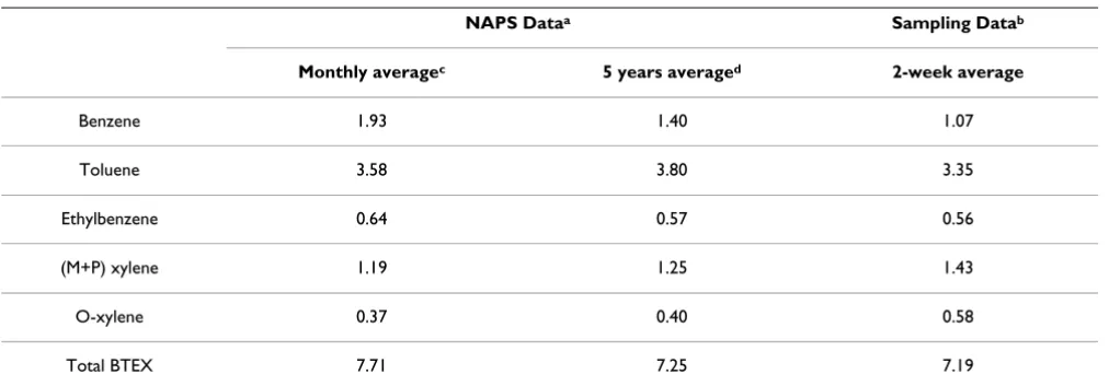
Table 2 compares monthly (there were only 4 measure-ments for the month of October 2005: 1st (Saturday), 7th (Friday), 19th (Wednesday), and 25th (Tuesday)) and 5-year (2001 – 2005) means of BTEX concentrations meas-ured at the National Air Pollution Surveillance (NAPS) station (#61004). The average ambient concentrations of the 3 sampling points closest to the station (Figure 1) were chosen for comparison following Atari et al. [55] and Miller et al. [47]. In general, the 2-week average concentra-tions of benzene (1.07 μg/m3), toluene (3.35 μg/m3), ethylbenzene (0.56 μg/m3), and total BTEX (7.19 μg/m3) at the 3 sampling points closest to the station were slightly lower than the monthly and 5-year means measured at the NAPS station (Table 2). The 2-week average concentra-tions of (m+p) xylene (1.43 μg/m3) and o-xylene (0.58
μg/m3) measured at the 3 sampling points closest to the station were slightly higher than the monthly and 5-year means measured at the NAPS station. The differences could be attributed to the fact that (m+p) xylene and o-xylene are more photochemically reactive than their coun-ter parts [57], and different measuring instruments were used. Environment Canada used 6 Litre Summa canisters at the NAPS stations [58] while 3 M samplers were used in this study.
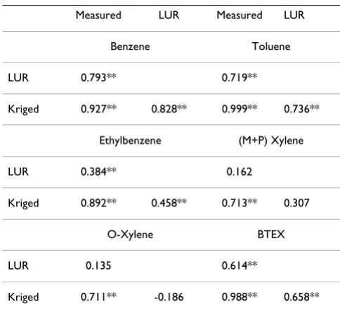
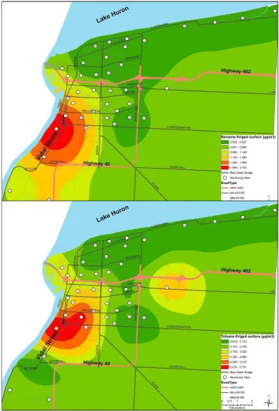
The measured BTEX species are highly correlated to each other (Table 3). The kriged surfaces of measured BTEX concentrations showed similar patterns with high concen-trations along the industrial core. Because of the high cor-relation between BTEX species and their similar patterns in the kriged surfaces, only two surfaces are shown (Figure 2). The benzene surface has a slightly more localized pat-tern when compared to the other BTEX species. Table 4 shows the Pearson correlation coefficients between meas-ured, kriged and LUR modelled concentrations at the sampling locations. The correlation between measured and kriged concentrations were low for ethylbenzene (r = 0.38), (m+p) xylene (r = 0.16) and o-xylene (0.14). Like-wise, the correlation between kriged and LUR modelled concentrations at the sampling locations were low for ethylbenzene (r = 0.46), (m+p) xylene (r = 0.31) and o-xylene (r = -0.19). Kriged o-o-xylene concentrations were consistently lower than the LUR modelled concentrations at the sampling locations.
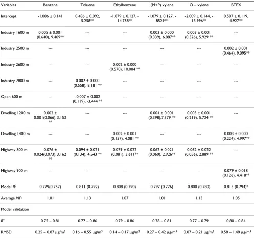
The calculated Moran's indices for benzene (MI = -0.02), toluene (MI = 0.01), ethylbenzene (MI = -0.04), (m+p) xylene (MI = -0.03), o-xylene (MI = -0.03), and total BTEX (MI = -0.03) residuals of the most predictive models indi-cate no significant autocorrelation. Table 5 shows the final LUR models for predicting the concentrations of benzene, toluene, ethylbenzene, (m+p) xylene, o-xylene, and total BTEX. The model for benzene (R2 = 0.78)
Table 1: Distribution of BTEX concentrations at measured sites
Percentiles
Mean SD Min Max 25th 50th 75th
Benzene 0.93 0.56 0.28 3.36 0.56 0.86 1.15
Toluene 2.58 1.35 0.85 6.88 1.67 2.20 3.42
Ethylbenzene 0.46 0.23 0.15 1.06 0.30 0.39 0.58
(M+P) xylene 1.21 0.61 0.40 2.81 0.78 1.08 1.56
O-xylene 0.49 0.25 0.15 1.19 0.32 0.43 0.63
included industrial land use within 1600 m, dwelling counts within 1200 m, and length of highway within 800 m. The model for toluene had an R2 of 0.81 including industrial land use within 2800 m, open area within 600 m, and length of highway within 800 m as significant pre-dictors. The model for ethylbenzene (R2 = 0.81) included industrial land within 2600 m, dwelling counts within 1400 m, and length of highway within 800 m. The model for (m+p) xylene and o-xylene had similar R2 of 0.80 including industrial land use within 1600 m, dwelling counts within 1200 m, and length of highway within 800 m. The total BTEX model had a coefficient of determina-tion (R2) of 0.81 including industrial land use within 2500 m, dwelling counts within 1400 m, and length of highway within 900 m showing significant contribution to the model. The positive regression coefficients indicate that concentrations of BTEX compounds increase as the values of the independent variables (e.g. industrial area) rise, while the negative coefficients indicate a decrease in concentrations as the values of the predictor variables (e.g. area of open space) increase. All variables in the six mod-els are significant at the 95% level of confidence. None of the variables in the final models were significantly corre-lated with each other (Table 6).
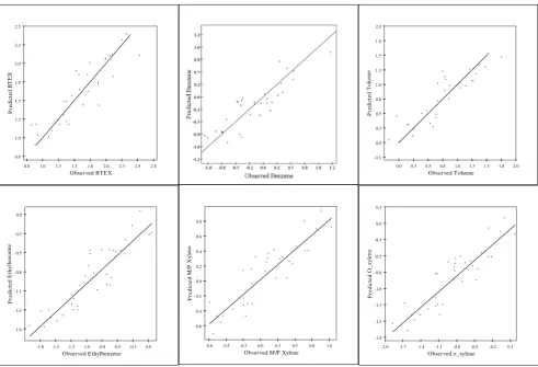
Figure 3 shows the relationship between the observed and predicted pollutants based on their natural logarithmic scales. The scatterplots reflect the strength of each of the developed models and demonstrate that the models fit the observations well with no significant outliers. The spa-tial pattern of the predicted BTEX species concentrations showed expected characteristics (Figure 4) compared to their kriged surfaces. The predicted surfaces reflected the significant variables with industrial area, dwelling counts
and traffic showing significance. The numerous petro-chemical industries along the industrial core and dwelling counts showed significant influences on the modelled surfaces. The predicted surfaces have more detailed varia-bility compared to the kriged surfaces of measured con-centrations.
The results of the validation approaches are provided in Table 5. The BTEX root mean square error predicted in this study were somewhat lower than the average estimated error of 1.72 – 2.15 μg/m3 for BTEX concentrations reported by Aquilera et al. [19] who used similar approaches for cross-validation. Overall, the predicted benzene, toluene, ethylbenzene, (m+p) xylene, o-xylene, and total BTEX concentrations correspond nicely with measured concentration suggesting that these models are capable of predicting reliable concentrations. The Chow test results were not significantly different between the predictive models and the three different tests suggesting that the benzene, toluene, ethylbenzene, (m+p) xylene, o-xylene and total BTEX models developed were quite sta-ble.
Discussion
The aim of this study was to model the intra-urban varia-tions of ambient VOCs including benzene, toluene, ethyl-benzene, (m+p) xylene, o-xylene, and total BTEX for use in a large health study aimed at examining the determi-nants of health in sentinel high exposure environments. Although most of the significant variables were similar in the six models, their individual contributions to the mod-els were significantly different. For example, while indus-trial land use within 1600 m was significant in both (m+p) xylenes and o-xylene models, the effect of industry
Table 2: Comparison between NAPS and sampled BTEX data
NAPS Dataa Sampling Datab
Monthly averagec 5 years averaged 2-week average
Benzene 1.93 1.40 1.07
Toluene 3.58 3.80 3.35
Ethylbenzene 0.64 0.57 0.56
(M+P) xylene 1.19 1.25 1.43
O-xylene 0.37 0.40 0.58
Total BTEX 7.71 7.25 7.19
a Measured data at the National Air Pollution Surveillance (NAPS); b 2-week average data at 3 sampling points closest to the NAPS station;
(34% and 53%, respectively) differed in the two models (Table 5). These differential influences support the need for modelling the different air pollutants [55].
When compared to other LUR models developed in Munich [59], El Paso [60], Sabadell [19] and Windsor, Ontario [61], the significant variables in the present study showed considerably larger buffer radii. For example, Wheeler et al. [61] reported significant highway buffer radii of 50 m and 100 m for benzene and toluene models, respectively. In this study, we found significant highway buffer radii of 800 m for both benzene and toluene mod-els (Table 5). The later result was also larger than the 300 m buffer radius reported by Beckerman et al. [62] when examining the variability of traffic-related pollutants around an expressway in Toronto, Ontario. The differ-ences could be due to the unusually large number of
pet-rochemical facilities in Chemical Valley, hence the broader distribution of ambient air pollutants in the area. The larger buffer radii found in this study potentially lim-its the generalizablility and transferability of the devel-oped LUR models to areas of similar contextual and compositional characteristics [26].
When compared to other models developed in Sabadell [19], Munich [59], and Windsor, Ontario [61], the results of the various models of BTEX species are considerably different, further suggesting the need to model air pollut-ants in their various contexts rather than depending on proxies [37,55]. The benzene model (R2 = 0.78) showed comparable coefficient of determination when compared to a similar model developed in Munich, Germany (R2 = 0.80) [59] but slightly higher than the R2 of a model devel-oped in Windsor, Ontario, Canada (R2 = 0.73) [61]. The toluene model showed high coefficient of determination (R2 = 0.81) compared to similar models developed in Windsor (R2 = 0.46) [61] and Munich (R2 = 0.76) [59], while the coefficient of ethylbenzene (R2 = 0.81) was com-parable to the coefficient reported in Munich (R2 = 0.79) [59]. The BTEX model developed in this study showed high coefficient of determination (R2 = 0.81) as compared to an R2 of 0.74 reported by Aquilera et al. [19] in Sabadell, Spain. Differences in the R2 could be due the contextual factors in the various cities. Although the industrial area exhibited varying influences in each of the models (Table 5), the results support the view that the numerous petrochemical industries are significantly affecting the VOC concentrations in Sarnia, Chemical Val-ley. If possible, it is important to model each air pollutant of interest to better analyse, determine, and understand personal exposures for health studies.
Besides industrial area, dwelling counts also emerged as a strong determinant of the intra-urban variation of BTEX concentration in Sarnia (Table 5). These results are con-sistent with other researchers [46] who found dwelling counts to influence the intra-urban variation of air
pollu-Table 3: Pearson correlation between measured ambient BTEX compounds
Toluene Ethylbenzene (M+P) xylene O-Xylene Total BTEX
Benzene 0.817** 0.845** 0.752** 0.755** 0.865**
Toluene 0.973** 0.965** 0.969** 0.991**
Ethylbenzene 0.977** 0.973** 0.989**
(M+P) xylene 0.994** 0.966**
O-Xylene 0.970**
** Significant at 95%
Table 4: Correlations between measured, kriged and LUR modelled concentrations at sampling locations in Sarnia
Measured LUR Measured LUR
Benzene Toluene
LUR 0.793** 0.719**
Kriged 0.927** 0.828** 0.999** 0.736**
Ethylbenzene (M+P) Xylene
LUR 0.384** 0.162
Kriged 0.892** 0.458** 0.713** 0.307
O-Xylene BTEX
LUR 0.135 0.614**
Kriged 0.711** -0.186 0.988** 0.658**
Kriged surfaces for measured benzene and toluene Figure 2
Kriged surfaces for measured benzene and toluene.
Figur e 2a: Benzene
tion. The view is that high dwelling counts may influence heavy traffic and emissions [63]. The results also indicate that a combination of land use and dwelling counts could be used to estimate exposure to air pollution, especially BTEX compounds.
The correlations between BTEX species in this study showed slightly different coefficient ranges compared to other studies in Canada and the US [62,64]. This research has slightly narrow coefficient ranges (0.76 – 0.99) (Table
3) compared to the coefficient ranges (0.53 – 0.89) reported in Toronto, Canada [62]. The difference could be due to the numerous petrochemical industries in the region. While examining the concentration and co-occur-rence of VOCs in the US, Pankow et al. [64] reported com-parable correlation ranges (0.78 – 0.99) between BTEX species. The high correlation coefficients in this study sug-gest that BTEX species are emitted by similar sources and it might be possible to monitor only one or two of BTEX species in Sarnia [47].
Table 5: Land use regression model results for BTEX compounds
Variables Benzene Toluene Ethylbenzene (M+P) xylene O – xylene BTEX
Intercept -1.086 ± 0.141 0.486 ± 0.092,
5.258**
1.879 ± 0.127, -14.758**
1.079 ± 0.127, -8529**
2.009 ± 0.144, -13.996**
0.587 ± 0.119, 4.927**
Industry 1600 m 0.005 ± 0.001 (0.640), 9.409**
--- --- 0.003 ± 0.000
(0.339), 6.887**
0.003 ± 0.001 (0.526), 5.929 **
---Industry 2500 m --- --- --- --- --- 0.002 ± 0.001
(0.464), 9.095**
Industry 2600 m --- --- 0.002 ± 0.000
(0.570), 10.084 **
--- ---
---Industry 2800 m --- 0.002 ± 0.000
(0.558), 8.181 **
--- --- ---
---Open 600 m --- -0.007 ± 0.002
(0.119), -3.444 **
--- --- ---
---Dwelling 1200 m 0.002 ±
0.001(0.066), 3.153 **
--- --- 0.004 ± 0.001
(0.398),7.379 **
0.003 ± 0.001 (0.219), 5.724 **
---Dwelling 1400 m --- --- 0.002 ± 0.001
(0.157), 4.081 **
--- --- 0.003 ± 0.000
(0.224), 4.997**
Highway 800 m 0.076 ±
0.024(0.073), 3.162 **
0.094 ± 0.021 (0.134), 4.543 **
0.079 ± 0.022 (0.081), 3.611**
0.062 ± 0.021 (0.060), 2.926**
0.062 ± 0.022 (0.056), 2.889 **
---Highway 900 m --- --- --- --- --- 0.079 ± 0.018
(0.126), 4.418**
Model R2 0.779(0.757) 0.811 (0.792) 0.808 (0.790) 0.797 (0.776) 0.800 (0.780) 0.813 (0.794)b
Average VIFc 1.01 1.13 1.07 1.01 1.13 1.05
Model validation
R2 0.75 – 0.81 0.77 – 0.86 0.79 – 0.86 0.78 – 0.81 0.77 – 0.79 0.80 – 0.84
RMSEd 0.25 – 0.87 μg/m3 0.16 – 0.55 μg/m3 0.14 – 0.17 μg/m3 0.27 – 0.42 μg/m3 0.07 – 0.21 μg/m3 0.58 – 1.48 μg/m3
Note: a C = coefficient, SE = Standard Error, Cont = R2 contribution; b Numbers in brackets are adjusted R2; c VIF = Variance Inflation Factor;
When compared to the measured concentrations (Table 4), kriging showed higher correlation coefficients (0.71 – 0.99) compared to the LUR modelled concentrations (0.14 – 0.79) for BTEX and all its individual components. The LUR models showed high correlations with measured concentrations for benzene (r = 0.79), toluene (r = 0.72), and BTEX (r = 0.61) but considerably lower correlation coefficients for ethylbenzene (r = 0.38), (m+p) xylene (0.16) and o-xylene (r = 0.14). When the kriged
concen-trations were compared to the LUR modelled concentra-tions at the monitoring sites, benzene (r = 0.83), toluene (r = 0.73), ethylbenzene (r = 0.51), and BTEX (r = 0.66) showed significantly higher correlations compared to (m+p) xylene (r = 0.31) and o-xylene (r = -0.19). The LUR models underestimated o-xylene concentration at the sampling locations compared to kriging. The correlation results suggest that LUR modelling could be an efficient interpolator for benzene, toluene, and ethylbenzene but
Table 6: Pearson correlation between significant variables in the most predictive LUR models
Benzene
Dwelling counts within 1200 m Length of highway within 800 m
Industrial Land Use within 1600 m 0.028 -0.058
Dwelling counts within 1200 m -0.056
Toluene
Open area within 600 m Length of highway within 800 m
Industrial Land Use within 2800 m -0.322 -0.164
Open area within 600 m -0.107
Ethylbenzene
Dwelling counts within 1400 m Length of highway within 800 m
Industrial Land Use within 2600 m 0.014 -0.205
Dwelling counts within 1400 m 0.221
(M+P) Xylene
Dwelling counts within 1200 m Length of highway within 800 m
Industrial Land Use within 1600 m 0.048 -0.119
Dwelling counts within 1200 m 0.042
O-Xylene
Dwelling counts within 1200 m Length of highway within 800 m
Industrial Land Use within 1600 m 0.042 -0.095
Dwelling counts within 1200 m -0.034
BTEX
Industrial land use Length of highway within 900 m
Dwelling counts within 1400 m 0.010 -0.179
not for xylenes in a highly polluted area like Sarnia. The effectiveness of kriging in Sarnia may be due to the uniqueness of the area. As mentioned, Sarnia is a rela-tively small region with about 40% of Canada's chemicals manufactured in the region [43].
Similar to other LUR studies, the benzene, toluene, ethyl-benzene, (m+p) xylene, o-xylene, and total BTEX models were developed based on a two-week monitoring cam-paign. The high network deployment, monitoring, and chemical analysis cost did not permit an extensive moni-toring campaign. In spite of the short-term monimoni-toring, the models developed captured the intra-urban variability of total BTEX and its associated species in Chemical Val-ley. When compared, the 2-week measured concentra-tions at the 3 sampling locaconcentra-tions closest to the National Air Pollution Surveillance (NAPS) station had compara-ble patterns with the monthly and 5-year average concen-trations at the station suggesting that the measured ambient BTEX concentrations in this study were reliable. Hence, although seasonal variations may affect the
tem-poral trend of modelled air pollution concentration, sea-sonality would have little influence on the spatial and geographic patterns of pollution because of the numerous petrochemical facilities in the region [53,55,63,65]. Sub-sequently, seasonal variation may not greatly influence chronic health outcomes because, as observed in this research, the 2-week concentrations adequately represent mean annual concentration in Sarnia (see also Lebret et al. [65])
Conclusion
Despite the potential limitations of this research, includ-ing the short-term monitorinclud-ing campaign, the develop-ment of LUR models is a relatively affordable approach that clearly offers an advantage over traditional exposure estimation methods such as dispersion models [35]. From the models developed, it is evident that in addition to industrial emissions, traffic related VOC pollutions can-not be ignored in Chemical Valley and in similar indus-trial areas. Because of their prevalence and potential to cause adverse health outcomes, it is crucial to model
Observed versus predicted BTEX, benzene, toluene, ethylbenzene, m/p xylene and o-xylene (logarithmic scale) based on the best land use regression models
Figure 3
Observed versus predicted BTEX, benzene, toluene, ethylbenzene, m/p xylene and o-xylene (logarithmic scale) based on the best land use regression models.
0.0 0.3 0.5 0.8 1.0 1.3 1.5 1.8 2.0 O bserved T oluene
-0.3 0.0 0.3 0.5 0.8 1.0 1.3 1.5 1.8 2.0 P re d ic te d T o lue ne > > > > > > >> > > > > > > > > > > > > > > >> > > > >> > > > >
-2.0 -1.7 -1.4 -1.1 -0.8 -0.5 -0.2 0.1 Observed o_xylene -1.8 -1.5 -1.3 -1.0 -0.8 -0.5 -0.3 0.0 0.3 P re d ic te d O _ x y le ne > > > > > > > > > > > > >> > > > > > > > > >> > >> > > > > > > > 0.8 1.0 1.3 1.5 1.8 2.0 2.3 2.5 2.8
Obser ved BTE X 0.8 1.0 1.3 1.5 1.8 2.0 2.3 2.5 P re d ic te d B T E X > > > > > > > > > > > > > > > > > > > > > > > > > > > > > > > >
-1.8 -1.5 -1.3 -1.0 -0.8 -0.5 -0.3 0.0 O bserved E thylbenzene -1.6 -1.4 -1.1 -0.8 -0.5 -0.3 0.0 P re d ic te d E th y lb e n ze ne > > > > > > > > > > > > > > > > > > > > > > > > > > > >
> > > > > >> -0.6 -0.4 -0.2 0.0 0.2 0.4 0.6 0.8 P re d ic te d M /P X y le ne > > > > > > > > > > > > > > > > > > > > > > > >> > > > > > > > >
VOCs such as BTEX for increasing the research communi-ties understanding of the link between air pollution and health. The modeled ambient air pollution surfaces gener-ated in this study suggest that some residents may be dis-proportionally exposed to high air pollutants. The results suggest the need for environmental policies that help reduce industrial pollution and assist residents to reduce and cope with daily industrial exposures. The LUR model-ling of benzene, toluene, ethylbenzene, (m+p) xylene, o-xylene, and total BTEX models are used to estimate per-sonal exposure for a large community health study aimed at examining the determinants of health in a government labelled area of concern.
Abbreviations
AADT: Annual average daily traffic; BTEX: Benzene, tolu-ene, ethylbenztolu-ene, m/p-xylene and o-xylene; DA: Dissem-ination area; DEMs: Digital elevation models; DMTI: Desktop Mapping Technologies Inc; GIS: Geographic Information Systems; HAP(s): Hazardous air pollutant(s); IARC: International Agency for Research on Cancer; LUR: Land use regression; MI: Moran I; NAPS: National Air Pol-lution Surveillance; NO2: Nitrogen dioxide; PM2.5: Fine particles (particles with diameter less than 2.5 μm); PM10: Particulate matter (particles with diameter less than 10
μm); RMSE: Root mean square error; VOC(s): Volatile organic compound(s); VMT: vehicle miles traveled.
Competing interests
The authors declare that they have no competing interests.
Authors' contributions
DA and IL conceived the study and were involved in the preparation of the manuscript. DA was involved in the analysis and interpretation of the results and preparation of the paper. All authors have read and approved the final manuscript.
Acknowledgements
The authors would like to thank the Ontario Ministry of Transportation for providing assistance in accessing the highways traffic count data, the City of Sarnia Works Administration and Engineering Department for providing the local daily traffic counts, and the Aamjiwnaang Indian Reserve for their support. The authors would also like to thank Dr. Iris Xu and her students at the University of Windsor for assisting in air quality data collection. We thank all the reviewers for their constructive suggestions and comments. This project is funded by the Social Sciences and Humanities Research Council of Canada grant (# 410-2004-0159) and Canada Research Chair funding to Dr. Luginaah.
References
1. Pratt GC, Palmer K, Wu CY, Oliaei F, Hollerbach C, Fenske MJ: An assessment of air toxics in Minnesota. Environ Health Perspect 2000, 108:815-825.
2. Woodruff TJ, Axelrad DA, Caldwell J, Morello-Frosch R, Rosenbaum
A: Public health implications of 1990 air toxics
concentra-tions across the United States. Environ Health Perspect 1998,
106:245-251.
Land use regression predicted surfaces for BTEX compounds Figure 4
3. Clean Air Act Amendments: Part A, Section 112. Public Law 1990:101-549.
4. Leikauf GD: Hazardous Air Pollutants and Asthma. Environ Health Perspect 2002, 110(S4):505-526.
5. Rumchev K, Spickett J, Bulsara M, Phillips M, Stick S: Association of domestic exposure to volatile organic compounds with asthma in young children. Thorax 2004, 59:746-751.
6. International Agency for Research on Cancer: IARC Monograph on the Evaluation of the Carcinogenic Risk of Chemicals: Some Industrial Chemi-cals and DyestuffsVolume 29. IARC: Lyon, France; 1982.
7. Lin M, Chen Y, Villeneuve PJ, Burnett RT, Lemyre L, Hertzman C, Mcgrail KM, Krewski D: Gaseous air pollutants and asthma hos-pitalization of children with low household income in Van-couver, British Columbia. Am J Epidemiol 2004, 159:294-303. 8. U.S. Department of Health and Human Services: The Agency for
Toxic Substances and Disease Registry (ATSDR). Toxicological Profile for Benzene 2007 [http://www.atsdr.cdc.gov/toxprofiles/ tp3.pdf].
9. Glass DC, Gray CN, Jolley DJ, Gibbons C, Sim MR, Fritschi L, Adams GG, Bisby JA, Manuell R: Leukemia risk associated with low-level benzene exposure. Epidemiology 2003, 14:569-577. 10. U.S. Department of Health and Human Services: The Agency for
Toxic Substances and Disease Registry (ATSDR). Toxicological Profile for Toluene 2000 [http://www.atsdr.cdc.gov/toxprofiles/tp3.pdf]. 11. Chang S, Chen C, Lien C, Sung F: Hearing Loss in Workers Exposed to Toluene and Noise. Environ Health Perspect 2006,
114:1283-1286.
12. Gerin M, Siemiatychi J, Desy M, Krewski D: Associations between several sites of cancer and occupational exposure to ben-zene, toluene, xylene, and styrene: results of a case-control study in Montreal. Am J Ind Med 1998, 34:144-156.
13. Antilla A, Pukkala E, Riala R, Sallmén M, Hemminki K: Cancer inci-dence among Finnish workers exposed to aromatic hydro-carbons. Int Arch Occup Environ Health 1998, 71:187-193. 14. International Agency for Research on Cancer: Monographs on the
evaluation of carcinogenic risks to humans. Xylenes. In Part Three. Re-evaluation of some organic chemicals, hydrazine, and hydrogen peroxide Volume 71. Lyon, France: World Health Organization; 1999:1189-1208.
15. Integrated Risk Information System: Benzene, Toluene, Ethylbenzene, and Xylenes Integrated Risk Information System, U.S. Environmental Protection Agency; 2001.
16. Vyskocil A, Leroux T, Truchon G, Lemay F, Gendron M, Gagnon F, El Majidi N, Viau C: Ethyl benzene should be considered ototoxic at occupationally relevant exposure concentrations. Toxicol-ogy and Industrial Health 2008, 24:241-246.
17. U.S. Environmental Protection Agency: Integrated Risk Information Sys-tem (IRIS) on Xylenes National Center for Environmental Assessment, Office of Research and Development, Washington, DC; 1999. 18. U.S. Department of Health and Human Services: The Agency for
Toxic Substances and Disease Registry (ATSDR). Toxicological Profile for Xylene (Update) 2007 [http://www.atsdr.cdc.gov/ tfacts71.pdf]. Atlanta, GA: U.S. Department of Public Health and Human Services, Public Health; Service
19. Aguilera I, Sunyer J, Fernandez-Patier R, Hoek G, Aguirre-Alfaro A, Meliefste K, Bomboi-Mingarro MR, Nieuwenhuijsen MJ, Herce-Garra-leta D, Brunekreef B: Estimation of outdoor NOx, NO2, and BTEX exposure in a cohort of pregnant women using land use regression modelling. Environ Sci Technol 2008, 42:815-821. 20. Sexton K, Adgate JL, Ramachandran G, Pratt GC, Mongin SJ, Stock
TH, Morandi MT: Comparison of personal, indoor, and out-door exposures to hazardous air pollutants in three urban communities. Environ Sci Technol 2004, 38:423-430.
21. Adgate JL, Church TR, Ryan AD, Ramachandran G, Fredrickson AL, Stock TH, Morandi MT, Sexton K: Outdoor, indoor, and personal exposure to VOCs in Children. Environ Health Perspect 2004,
112:1386-1392.
22. Lee S: Comparison of indoor and outdoor air quality at two staff quarters in Hong Kong. Environ Int 1997, 23(6):791-797. 23. Rava M, Verlato G, Bono R, Ponzio M, Sartori S, Blengio G, Kuenzli
N, Heinrich J, Götschi T, de Marco R: A predictive model for the home outdoor exposure to nitrogen dioxide. Sci Total Environ 2007, 384:163-170.
24. Brunekreef B, Holgate ST: Air pollution and health. Lancet 2002,
360:1233-1242.
25. Pope CA, Dockery DW: Health effects of fine particulate air pollution: lines that connect. J Air Waste Manag Assoc 2006,
56:709-742.
26. Hoek G, Beelen R, de Hooh K, Vienneau D, Gulliver PF, Briggs D: A review of land use regression models to assess spatial
varia-tion of outdoor air polluvaria-tion. Atmos Environ 2008,
42(33):7561-7578.
27. Ryan P, LeMasters G: A review of land-use regression models for characterising intraurban air pollution exposure. Inhal Toxicol 2007, 19(Suppl 1):127-133.
28. Briggs D: The role of GIS: coping with space (and time) in air pollution exposure assessment. J Toxicol Environ Health A 2005,
68:1243-1261.
29. Dockery DW, Stone PH: Cardiovascular risks from fine partic-ulate air pollution. N Eng J Med 2007, 356:511-513.
30. Burnett RT, Stieb D, Brook JR, Cakmak S, Dales R, Raizenne M, Vin-cent R, Dann T: Associations between short-term changes in nitrogen dioxide and mortality in Canadian cities. Arch Environ Health 2004, 59:228-236.
31. Pope CA, Burnett RT, Thun MJ, Calle EE, Krewski D, Ito K, Thurston
GD: Lung cancer, cardiopulmonary mortality, and long-term
exposure to fine particulate air pollution. J Am Med Assoc 2002,
287:1132-1141.
32. Jerrett M, Arain A, Kanaroglou P, Beckerman B, Crouse D, Gilbert NL, Brook JR, Finkelstein N, Finkelstein MM: Modelling the intra-urban variability of ambient traffic pollution in Toronto, Canada. J Toxicol Environ Health A 2007, 70:200-212.
33. Levy J, Houseman EA, Ryan L, Richardson D, Spengler JD: Particle
concentration in urban microenvironments. Environ Health
Persp 2000, 108:1051-1057.
34. Madsen C, Carlsen KC, Hoek G, Oftedal B, Nafstad P, Meliefste K, Jacobsen R, Nystad W, Carlsen K, Brunekreef B: Modelling the intra-urban variability of outdoor traffic pollution in Oslo, Norway–A GA2 LEN project. Atmos Environ 2007, 41:7500-7511. 35. Jerrett M, Arain A, Kanaroglou P, Beckerman B, Potoglou D, Sahsu-varoglu T, Morrison J, Giovis C: A review and evaluation of intra-urban air pollution exposure models. J Expo Anal Environ Epide-miol 2005, 15:185-204.
36. Briggs D, Collins S, Elliott P, Kingham S, Lebret E, Pryl K, van Reeuwijk H, Smallbone K, Laan A van der: Mapping urban air pollution using GIS: a regression-based approach. Int J Geogr Information Syst 1997, 11:699-718.
37. Ryan P, LeMasters G, Biswas P, Levin L, Hu S, Lindsey M, Bernstein D, Lockey J, Villareal M, Hershey GK, Grinshpun SA: A comparison of proximity and land use regression traffic exposure models
and wheezing in infants. Environ Health Perspect 2006,
115:278-284.
38. Fischer P, Hoek G, van Reeuwijk H, Briggs DJ, Lebret E, van Wijnen JH, Kingham S, Elliott P: Traffic-related differences in outdoor and indoor concentrations of particles and volatile organic compounds in Amsterdam. Atmos Environ 2000, 34:3713-3722. 39. Linaker C, Chauhan A, Inskip H, Holgate S, Coggon D: Personal
exposures of children to nitrogen dioxide relative to concen-trations in outdoor air. J Occup Environ Med 2000, 57:472-476. 40. Fung K, Luginaah I, Gorey K: Impact of air pollution on hospital
admissions in Southwestern Ontario, Canada: Generating hypotheses in sentinel high-exposure places. Environ Health 2007, 6:18.
41. Brauer M, Hoek G, van Vliet P, Meliefste K, Fischer P, Gehring U, Heinrich J, Cyrys J, Bellander T, Lewne M, Brunekreef B: Estimating long-term average particulate air pollution concentrations: application of traffic indicators and geographic information systems. Epidemiology 2003, 14:228-239.
42. Statistics Canada: 2006 Community Profiles [http://www12.statcan.ca/ english/census06/data/profiles/community/Index.cfm?Lang=E]. 43. Gilbertson M, Brophy J: Community health profile of Windsor,
Ontario, Canada: anatomy of a great lakes area of concern.
Environ Health Persp 2001, 109(Suppl 6):827-843.
44. Curren KC, Dann TF, Wang DK: Ambient air 1,3-butadiene con-centration in Canada (1995–2003): seasonal, day of week var-iations, trends, and source influences. Atmos Environ 2006,
40:171-181.
45. Health Canada: Health Data and Statistics Compilations for Great Lakes Areas of Concern Health Canada, Ottawa, Ontario; 2000.
net-Publish with BioMed Central and every scientist can read your work free of charge
"BioMed Central will be the most significant development for disseminating the results of biomedical researc h in our lifetime."
Sir Paul Nurse, Cancer Research UK
Your research papers will be:
available free of charge to the entire biomedical community
peer reviewed and published immediately upon acceptance
cited in PubMed and archived on PubMed Central
yours — you keep the copyright
Submit your manuscript here:
http://www.biomedcentral.com/info/publishing_adv.asp
BioMedcentral
work for intra-urban population exposure assessment: A location-allocation approach. Atmos Environ 2005, 39:2399-2409. 47. Miller L, Xu X, Luginaah I: Spatial variability of VOC concentra-tions in Sarnia, Ontario, Canada. J Toxicol Environ Health A 2009,
72:1-15.
48. SPSS 15.0 for Windows. SPSS Inc. Headquarters, 233 S. Wacker Drive, 11th floor, Chicago, IL 60606 2007.
49. Hamilton L: Regression with Graphics: A Second Course in Applied Statis-tics Duxbury Press: Belmont, California; 1992.
50. Odland J: Spatial Autocorrelation Sage Publications: New Delhi, India; 1998.
51. Griffith DA: Spatial Autocorrelation: A Primer Resource publications in geography. Association of American Geographers, Washington, DC; 1987.
52. Isaaks E, Srivastava R: An Introduction to Applied Geostatistics Oxford University Press: New York, NY; 1989.
53. Sahsuvaroglu T, Arain A, Kanaroglou PS, Finkelstein N, Newbold B, Jerrett M, Beckerman B, Brook JR, Finkelstein M, Gilbert NL: A land use regression model for predicting ambient concentrations of nitrogen dioxide in Hamilton, Ontario, Canada. J Air Waste Manag Assoc 2006, 56:1059-1069.
54. Chow G: Tests of equality between sets of coefficients in two linear regressions. Econometrica 1960, 28:591-605.
55. Atari DO, Luginaah I, Xu X, Fung K: Spatial variability of ambient nitrogen dioxide and sulphur dioxide in Sarnia, "Chemical Valley", Ontario, Canada. J Toxicol Environ Health A 2008, 71:1-10. 56. Gilbert NL, Goldberg MS, Beckerman B, Brook JR, Jerrett M: Assess-ing Spatial Variability of Ambient Nitrogen Dioxide in Mon-treal, Canada, with a Land-Use Regression Model. J Air Waste Manag Assoc 2005, 55(8):1059-1063.
57. Monod A, Sive BC, Avino P, Chen T, Blake DB, Rowland FS: Monoar-omatic compounds in ambient air of various cities: a focus on
correlations between the xylenes and ethylbenzene. Atmos
Environ 2001, 35:135-149.
58. Environment Canada: National Air Pollution Surveillance
(NAPS) Network. 2001 [http://www.etc-cte.ec.gc.ca/NAPS/
naps_summary_e.html]. NAPS Network Summary
59. Carr D, von Ehrestein O, Weiland S, Wagner C, Wellie O, Nicolai T, von Mutius E: Modelling annual benzene, toluene, NO2, and soot concentrations on the basis of road traffic characteris-tics. Environ Res Sect 2002, 90:111-118.
60. Smith L, Mukerjee S, Gonzales M, Stallings C, Neas L, Norris GH: Use of GIS and ancillary variables to predict volatile organic com-pound and nitrogen dioxide levels at unmonitored locations.
Atmos Environ 2006, 40:3773-3787.
61. Wheeler AJ, Smith-Doiron M, Xu X, Gilbert NL, Brook JR: Intra-urban variability of air pollution in Windsor, Ontario-meas-urement and modeling for human exposure assessment.
Environ Res 2008, 106:7-16.
62. Beckerman B, Jerrett M, Brook JR, Verma DK, Arain MA, Finkelstein MM: Correlation of nitrogen dioxide with other traffic pollut-ants near a major expressway. Atmos Environ 2008, 42:275-290. 63. Ross Z, English PB, Scalf R, Gunier R, Smorodinsky S, Wall S, Jerrett
M: Nitrogen dioxide prediction in Southern California using
land use regression modeling: potential for environmental health analyses. J Expo Sci Environ Epidemiol. 2006 Mar;16(2):106-14 2006, 16(2):106-114.
64. Pankow JF, Luo W, Bender DA, Isabelle LM, Hollingsworth JS, Chen C, Asher WE, Zogorski JS: Concentration and co-occurrence correlations of 88 volatile organic compounds (VOC) in the ambient air of 13 semi-rural to urban locations in the United States. Atmos Environ 2003, 37:5023-5046.