Timed Consistent Network Updates
Tal Mizrahi, Efi Saat, Yoram Moses
∗Technion — Israel Institute of Technology
{dew@tx, efisaat@tx, moses@ee}.technion.ac.il
Abstract
Network updates such as policy and routing changes occur frequently in Software Defined Networks (SDN). Updates should be performed consistently, preventing temporary dis-ruptions, and should require as little overhead as possible. Scalability is increasingly becoming an essential requirement in SDN. In this paper we propose to use time-triggered net-work updates to achieve consistent updates. Our proposed solution requires lower overhead than existing update ap-proaches, without compromising the consistency during the update. We demonstrate that accurate time enables far more scalable consistent updates in SDN than previously available. In addition, it provides the SDN programmer with fine-grained control over the tradeoff between consistency and scalability.
Categories and Subject Descriptors
C.2.3 [Computer-Communication Networks]: Network Operations
Keywords
SDN, PTP, IEEE 1588, clock synchronization, management, time.
1.
INTRODUCTION
1.1
Background
Traditional network management systems are in charge of initializing the network, monitoring it, and allowing the op-erator to apply occasional changes when needed. Software Defined Networking (SDN), on the other hand, requires a central controller to routinely perform frequent policy and configuration updates in the network.
The centralized approach used in SDN introduces challenges in terms ofconsistencyandscalability. The controller must
∗
The Israel Pollak academic chair at Technion.
Permission to make digital or hard copies of all or part of this work for personal or classroom use is granted without fee provided that copies are not made or distributed for profit or commercial advantage and that copies bear this notice and the full citation on the first page. To copy otherwise, to republish, to post on servers or to redistribute to lists, requires prior specific permission and/or a fee.
SOSR2015,June 17 - 18, 2015, Santa Clara, CA, USA
take care to minimize network anomalies during update pro-cedures, such as packet drops or misroutes caused by tempo-raryinconsistencies. Updates must also be planned with scalabilityin mind; update procedures must scale with the size of the network, and cannot be too complex. In the face of rapid configuration changes, the update mechanism must allow a high update rate.
Two main methods for consistent network updates have been thoroughly studied in the last few years.
• Ordered updates. This approach uses a sequence of configuration commands, whereby theorder of execution guarantees that no anomalies are caused in intermediate states of the procedure [11, 18, 45, 24]; at each phase the controller waits until all the switches have completed their updates, and only then invokes the next phase in the sequence.
• Two-phase updates. In the two-phase approach [42, 20], configuration version tags are used to guarantee con-sistency; in the first phase the new configuration is in-stalled in all the switches in the middle of the network, and in the second phase the ingress switches are instructed to start using a version tag that represents the new config-uration. During the update procedure every switch main-tains two sets of entries: one for the old configuration version, and one for the new version. The version tag at-tached to the packet determines whether it is processed according to the old configuration or the new one. Af-ter the packets carrying the old version tag are drained from the network, garbage collection is performed on the switches, removing the duplicate entries and leaving only the new configuration.
In previous work [29] we argued that time is a powerful abstraction for coordinating network updates. We defined an extension [33] to the OpenFlow protocol [39] that al-lows time-triggered operations. This extension has been ap-proved and integrated into OpenFlow 1.5 [41], and into the OpenFlow 1.3.x extension package [40].
1.2
Time for Consistent Updates
ap-proach, where each of the two phases is invoked at a different time.
We show how theorder and two-phase approaches benefit from time-triggered phases. Contrary to the conventional order andtwo-phase approaches, timed updates do not re-quire the controller to wait until a phase is completed before invoking the next phase, significantly simplifying the con-troller’s involvement in the update process, and reducing the update duration.
The time-based method significantly reduces the time dura-tion required by the switches to maintain duplicate policy rules for the same flow. In order to accommodate the du-plicate policy rules, switch flow tables should have a set of spare flow entries [42, 20] that can be used for network up-dates. Timed updates use each spare entry for a shorter duration than untimed updates, allowing higher scalability.
Accurate time synchronization has evolved over the last decade, as the Precision Time Protocol (PTP) [16] has be-come a common feature in commodity switches, allowing sub-microsecond accuracy in practical use cases (e.g., [4]). However, even if switches have perfectly synchronized clocks, it is not guaranteed that updates areexecuted at their sched-uled times. We argue that a carefully designed switch can schedule updates with a high degree of accuracy. Moreover, we show that even if switches are not optimized for accurate scheduling, then the timed approach outperforms conven-tional update approaches.
The use of time-triggered updates accentuates a tradeoff between updatescalability andconsistency. At one end of the scale, consistent updates come at the cost of a poten-tially long update duration, and expensive memory waste due to rule duplication.1 At the other end, a
network-wide update can be invoked simultaneously, using Time-Conf[29], allowing a short update time, preventing the need for rule duplication, but yielding a brief period of inconsis-tency. In this paper we show that timed updates can be tuned to any intermediate point along this scale.
1.3
Contributions
The main contributions of this paper are as follows.
• We propose to use time-triggered network updates in a way that requires a lower overhead than existing update approaches without compromising the consistency during the update.
• We show that timed consistent updates require a shorter duration than existing consistent update methods.
• We define an inconsistency metric, allowing to quantify how consistent a network update is.
1As shown in [20], thedurationof an update can be traded
for the update rate. The flow table will typically include a limited number of excess entries that can be used for dupli-cated rules. By reducing the update duration, the excess en-tries are used for a shorter period of time, allowing a higher number of updates per second.
• We show that accurate time provides the SDN program-mer with a knob for fine-tuning the tradeoff between con-sistency and scalability.
• We present an experimental evaluation on a 50-node testbed, demonstrating the significant advantage of timed updates over other update methods.
For the sake of brevity, proofs have been omitted from this paper, and are presented in [35].
2.
TIME-BASED CONSISTENT UPDATES
We now describe the concept of time-triggered consistent up-dates. We assume that switches keep local clocks that are synchronized to a central reference clock by a synchroniza-tion protocol, such as the Precision Time Protocol (PTP) [16] orReversePTP[32, 31], or by an accurate time source such as GPS. The controller sends network update messages to switches using an SDN protocol such as OpenFlow [41]. An update message may specifywhen the corresponding update is scheduled to be performed.
S2 S1
S3 S4 after before
1 2
3
(a) Ordered update of a path.
S2 S1
S3
1 2
3
S4
(b) Two-phase update of a multicast distribution tree.
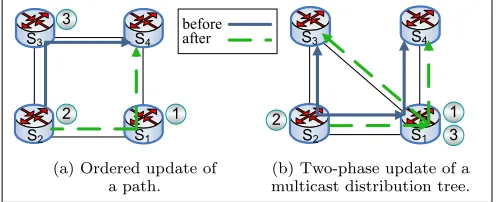
Figure 1: Update procedure examples.
2.1
Ordered Updates
Fig. 1a illustrates an ordered network update. We would like to reconfigure the path of a traffic flow from the ‘before’ to the ‘after’ configuration. An ordered update proceeds as described in Fig. 2; the phases in the procedure correspond to the numbers in Fig. 1a.
Untimed Ordered Update
1 Controller sends the ‘after’ configuration toS1.
2 Controller sends the ‘after’ configuration toS2.
3 Controller updatesS3 (garbage collection).
Figure 2: Ordered update procedure for the scenario of Fig. 1a.
The ordered update procedure guarantees that if every phase is performed after the previous phase was completed, then no packets are dropped during the process. Atime-based order update procedure is described in Fig. 3.
Timed Ordered Update
0 Controller sends timed updates to all switches. 1 S1 enables the ‘after’ configuration at timeT1.
2 S2 enables the ‘after’ configuration at timeT2> T1.
3 S3 performs garbage collection at timeT3 > T2.
Figure 3: Timed Ordered update procedure for the scenario of Fig. 1a.
phase 0, and ifT1 is timed correctly, the update process is
not influenced by these issues.
2.2
Two-phase Updates
An example of atwo-phase update is illustrated in Fig. 1b; the figure depicts a multicast distribution tree through a network of three switches. Multicast packets are distributed along the paths of the ‘before’ tree. We would like to recon-figure the distribution tree to the ‘after’ state.
Untimed Two-phase Update
1 Controller sends the ‘after’ configuration toS1.
2 Controller instructsS2 to start using the ‘after’
configuration with the new version tag. 3 Controller updatesS1 (garbage collection).
Figure 4: Two-phase update procedure for the scenario of Fig. 1b.
Thetwo-phase procedure [42, 20] is described in Fig. 4. In the first phase, the new configuration is installed inS1,
in-structing it to forward packets that have the new version tag according to the ‘after’ configuration. In the second phase, S2 is instructed to forward packets according to the ‘after’
configuration using the new version tag. The ‘before’ con-figuration is removed in the third phase. As in the ordered approach, thetwo-phase procedure requires every phase to be invoked after it is guaranteed that the previous phase was completed.
Timed Two-phase Update
0 Controller sends timed updates to all switches. 1 S1 enables the ‘after’ configuration at timeT1.
2 S2 enables the ‘after’ configuration with the
new version tag at timeT2> T1.
3 S1 performs garbage collection at timeT3 > T2.
Figure 5: Timed two-phase update procedure for the sce-nario of Fig. 1b.
In the timedtwo-phaseapproach, specified in Fig. 5, phases 1, 2, and 3 are scheduled in advance by the controller. The switches then execute phases 1, 2, and 3 at times T1, T2,
andT3, respectively.
2.3
k-Phase Consistent Updates
The order approach guarantees consistency if updates are performed according to a specific order. More generally, we can view an ordered update as a sequence ofkphases, where in each phase j, a set ofNj switches is updated. For each phasej, the updates of phase jmust be completed before any update of phasej+ 1 is invoked.
Thetwo-phase approach is a special case, wherek = 2; in the first phase all the switches in the middle of the network are updated with the new policy, and in the second phase the ingress switches are updated to start using the new version tag.
2.4
The Overhead of Network Updates
Both the order method and thetwo-phase method require duplicate configurations to be present during the update procedure. In each of the protocols of Fig. 2-5, both the ‘be-fore’ and the ‘after’ configurations are stored in the switches’ expensive flow tables from phase 1 to phase 3. The unnec-essary entries are removed only after garbage collection is performed in phase 3.
In the timed protocols of Fig. 3 and 5 the switches receive the update messages in advance (phase 0), and can temporar-ily store the new configurations in a non-expensive mem-ory. The switches install the new configuration in the ex-pensive flow table memories only at the scheduled times, thereby limiting the period of duplication to the duration from phase 1 to phase 3.
The overhead cost of the duplication depends on the time elapsed between phase 1 and phase 3. Hence, throughout the paper we use theupdate durationas a metric for quantifying the overhead of a consistent update that includes a garbage collection phase.
3.
TERMINOLOGY AND NOTATIONS
3.1
The Network Model
We reuse some of the terminology and notations of [42]. Our system consists ofN+1 nodes: a controllerc, and a set ofN switches, S={S1, . . . , SN}. Apacket is a sequence of bits, denoted bypk∈Pk, wherePkis the set of possible packets in the system. Every switchSi∈Shas a setPriof ports.
The sources and destinations of the packets are assumed to be external; packets are received from the ‘outside world’ through a subset of the switches’ ports, referred to asingress ports. Aningress switch is a switch that has at least one ingress port. Every packet pk is forwarded through a se-quence of switches (Si1, . . . , Sim), where the first switchSi1 is an ingress switch. The last switch in the sequence, Sim, forwards the packet through one of its ports to the outside world.
When a packet pk is received by a switchSi through port
It is assumed that every switch maintains a local clock. As is standard in the literature (e.g., [23]), we distinguish between real time, an assumed Newtonian time frame that is not directly observable, andlocal clock time, which is the time measured on one of the switches’ clocks. We denote values that refer to real time by lowercase letters, e.g. t, and values that refer to clock time by uppercase, e.g.,T.
We define apacket instanceto be a tuple (pk, Si, p, t), where
pk ∈ Pk is a packet, Si ∈ S is the ingress switch through which the packet is received,p∈Pri is the ingress port at switchSi, andtis the time at which the packet instance is received bySi.
3.2
Network Updates
We define asingleton update uof switchSi to be a partial function,u:Pk×Pri*A. A switch applies a singleton up-date,u, by replacing its forwarding function,Fiwith a new forwarding function,F0i, that behaves likeu in the domain ofu, and likeFi otherwise. We assume that every singleton update is triggered by a set of one or more messages sent by the controller tooneof the switches.
We define anupdateU to be a set of singleton updatesU =
{u1, . . . , um}.
We define an update procedure, U, to be a set U =
{(u1, t1, phase(u1)), . . . ,(um, tm, phase(um))} of 3-tuples, such that for all 1 ≤j ≤m, we have thatuj is a single-ton update, phase(uj) is a positive integer specifying the phase number of uj, and tj is the time at which uj is per-formed. Moreover, it is required that for every 1≤i, j≤m ifphase(ui) < phase(uj) thenti < tj. This definition im-plies that an update procedure is a sequence of one or more phases, where each phase is performed after the previous phase is completed, but there is no guarantee about the or-der of the singleton updates of each phase.
A k-phase update procedure is an update procedure U =
{(u1, t1, phase(u1)), . . . ,(um, tm, phase(um))} in which for all 1 ≤ j ≤ m we have 1 ≤ phase(uj) ≤ k, and for all 1≤i≤kthere exists an updateujsuch that (uj, tj, i)∈U.
We define a timed singleton update uT to be a pair (u, T), where u is a singleton update, and T is a clock value that represents the scheduled time of u. We as-sume that every switch maintains a local clock, and that when a switch receives a message indicating a timed sin-gleton update uT it implements the update as close as possible to the instant when its local clock reaches the value T. Similar to the definition of an update proce-dure, we define a timed update procedure UT to be a set UT ={(uT1, t1, phase(u1)), . . . ,(uTm, tm, phase(um))}.
An update procedure U =
{(u1, t1, phase(u1)), . . . ,(um, tm, phase(um))}
and a timed update procedure UT =
{(vT1, t1, phase(vT1)), . . . ,(vTn, tn, phase(vTn))} = {((v1, T1), t1, phase(vT1)), . . . ,((vn, Tn), tn, phase(vTn))} are said to be similar, denoted by UT ∼ U if m = n and for every 1 ≤ j ≤ m we have uj = vj and
phase(uj) =phase(vj).
Given anuntimed update,U, the original configuration, be-fore any of the singleton updates ofU takes place, is given by the set of forwarding functions,{F1, . . . ,FN}. We denote the new configuration, after all the singleton updates of U have been implemented, by{F01, . . . ,F
0
N}.
We define consistent forwarding based on the per-packet consistency definition of [42]. Intuitively, a packet is con-sistently forwarded if it is processed either according to the new configuration or according to the old one, but not ac-cording to a mixture of the two. Formally, let (pk, Si1, p1, t) be a packet instance that is forwarded through a sequence of switches Si1, Si2, . . . , Sim through ports p1, p2, . . . , pm, re-spectively, and is assigned the actions a1, a2, . . . , am. The packet instance (pk, Si1, p1, t) is said to beconsistently
for-warded if one of the following is satisfied:
(i)Fij(pk, pj) =ajfor all 1≤j≤m, or
(ii)F0ij(pk, pj) =ajfor all 1≤j≤m.
A packet instance that is not consistently forwarded, is said to beinconsistently forwarded.
Dc An upper bound on the controller-to-switch delay, including the network latency, and the internal switch delay until completing the up-date.
Dn An upper bound on the end-to-end network delay.
∆ An upper bound on the time interval between the transmission times of two consecutive up-date messages sent by the controller.
δ An upper bound on the scheduling error; an update that is scheduled to be performed atT is performed in practice during the time inter-val [T, T +δ].
Tsu The timed update setup time; in order to in-voke a timed update that is scheduled to time T, the controller sends the update messages no later than atT−Tsu.
Table 1: Delay-related Notations
3.3
Delay-related Notations
Table 1 presents key notations related to delay and perfor-mance. The attributes that play a key role in our analysis are Dc, Dn, andδ. These attributes are discussed further in Section 4.
4.
UPPER AND LOWER BOUNDS
4.1
Delay Upper Bounds
Both theorder and thetwo-phase approaches implicitly as-sume the existence of two upper bounds, Dc and Dn (see Table 1):
procedure. Alternatively, explicit acknowledgments can be used to indicate update completions; when a switch completes the update it notifies the controller. Unfortu-nately, OpenFlow [41, 26] currentlydoes notsupport such an acknowledgment mechanism. Hence, one can either use other SDN protocols that support explicit acknowl-edgment (as was assumed in [18]), or wait for a period of Dcuntil the switch is guaranteed to complete the update. • Dn: garbage collection can take place after the update procedure has completed, and all en-route packets have been drained from the network. Garbage collection can be invoked either after waiting for a period of Dn after completing the update, or by usingsoft timeouts.2 Both
of these approaches assume there is an upper bound,Dn, on the end-to-end network latency.
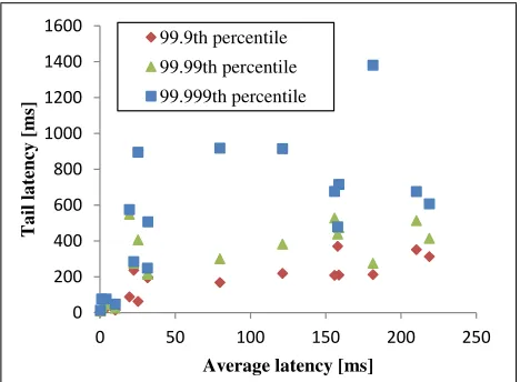
Is it practical to assume that the upper boundsDc andDn exist? Network latency is often modeled using long-tailed distributions such as exponential or Gamma [37, 13], imply-ing that network latency is oftenunbounded.
We demonstrate the long-tailed behavior of network latency by analyzing measurements performed on production net-works. We analyze 20 delay measurement datasets from [6, 2] taken at various sites over a one-year period, from Novem-ber 2013 to NovemNovem-ber 2014. 3 The measurements cap-ture the round-trip time (RTT) using ICMP Echo requests. The measurements show (Fig. 6) that in some networks the 99.999th percentile is almost two orders of magnitude higher than the average RTT. Table 2 summarizes the ra-tio between tail latency values and average values in the 20 traces we analyzed.
0 200 400 600 800 1000 1200 1400 1600
0 50 100 150 200 250
T
a
il
l
a
te
n
cy
[
m
s]
Average latency [ms]
99.9th percentile 99.99th percentile 99.999th percentile
Figure 6: Long-tail latency
In typical networks we expectDnto have long-tailed behav-ior. Similar long-tailed behavior has also been shown forDc in [18, 43].
2Soft timeouts are defined in the OpenFlow protocol [41] as a
means for garbage collection; a flow entry that is configured with a soft timeout,Dn, is cleared if it has not been used for a durationDn.
3Details about the measurements can be found in
Ap-pendix A.
99.9th percentile
99.99th percentile
99.999th percentile
4.88 10.49 19.45
Table 2: The mean ratio between the tail latency and the average latency.
At a first glance, these results seem troubling: if network latency is indeed unbounded, neither theorder nor the two-phase approaches can guarantee consistency, since the con-troller can never be sure that the previous phase was com-pleted before invoking the next phase.
In practice, typical approaches will not require a true upper bound, but rather a latency value that is exceeded with a sufficiently low probability. Service Level Agreement (SLA) in carrier networks is a good example of this approach; per the MEF 10.3 specification [27], a Service Level Specifica-tion (SLS) defines not only the mean delay, but also the Frame Delay Range (FDR), and the percentile defining this range. Thus, service providers must guarantee that the rate of frames that exceed the delay range is limited to a known percentage.
Throughout the paper we useDc andDn, referring to the upper bounds of the delays. In practice, these may refer to a sufficiently high percentile delay. Our analysis in Section 6 revisits the upper bound assumption.
4.2
Delay Lower Bounds
Throughout the paper we assume that the lower bounds of the network delay and the controller-to-switch delay are zero. This assumption simplifies the presentation, although the model can be extended to include non-zero lower bounds on delays.
4.3
Scheduling Accuracy Bound
As defined in Table 1,δis an upper bound on the scheduling error, indicating how accurately updates are scheduled; an update that is scheduled to take place at timeTis performed in practice during the interval [T, T+δ].4 A switch’s schedul-ing accuracy depends on two factors: (i) how accurately its clock is synchronized to the system’s reference clock, and (ii) its ability to perform real-time operations.
Most high-performance switches are implemented as a com-bination of hardware and software components. A schedul-ing mechanism that relies on the switch’s software may be affected by the switch’s operating system and by other run-ning tasks, consequently affecting the scheduling accuracy. Furthermore, previous work [18, 43] has shown high vari-ability in rule installation latencies in Ternary Content Ad-dressable Memories (TCAMs), resulting from the fact that a TCAM update might require the TCAM to be rearranged.
Nevertheless, existing switches and routers practice real-time behavior, with a predictable guaranteed response real-time to important external events. Traditional protection switch-ing and fast reroute mechanisms require the network to react
4An alternative representation of δ assumes a symmetric
Ck,N-2
Ck,N-1
Ck,N Sk,N-2
Sk,N-1
Sk,N
Cfin
0
0
0 Dc
Dc
Dc
Phase k Dc
C1,1
C1,2
C1,3 S1,1
S1,2
S1,3
C2,4
C2,5
C2,6 S2,4
S2,5
S2,6 Dc
Dc
0 0
0
0
0
0 Dc
Dc
Dc
Phase 1 Phase 2
0 Cstart
max( ,Dc) max( ,Dc)
C3,1
...
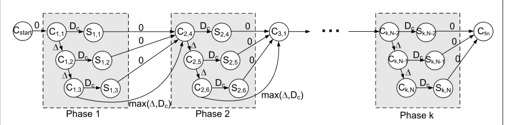
Figure 7: PERT graph of ak-phase update.
to a path failure in less than 50 milliseconds, implying that each individual switch or router reacts within a few millisec-onds, or in some cases less than one millisecond (e.g. [38]). Operations, Administration, and Maintenance (OAM) pro-tocols such as the IEEE 802.1ag [1] require faults to be de-tected within a strict timing constraint of ±0.42 millisec-onds.5
Measures can be taken to implement accurate scheduling of timed updates:
• Common real-time programming practices can be applied to ensure guaranteed performance for time-based update, by assigning a constant fraction of time to timed updates.
• When a switch is aware of an update that is scheduled to take place at time Ts, it can avoid performing heavy maintenance tasks near this time, such as TCAM entry rearrangement.
• Untimed update messages received slightly before timeTs can be queued and processed after the scheduled update is executed.
• If a switch receives a time-based command that is sched-uled to take place at the same time as a previously received command, it can send an error message to the controller, indicating that the last received command cannot be ex-ecuted.
• It has been shown that timed updates can be scheduled with a very high degree of accuracy, on the order of 1 mi-crosecond, using TimeFlip[34]. This approach provides a high scheduling accuracy, potentially at the cost of some overhead in the switch’s flow tables.
Observation 1. In typical settingsδ < Dc.
The intuition behind Observation 1 is thatδis only affected by the switch’s performance, whereasDcis affected by both the switch’s performance and the network latency. We ex-pect Observation 1 to hold even if switches are not designed for real-time performance. We argue that in switches that
5
Faults are detected using Continuity Check Messages (CCM), transmitted every 3.33 ms. A fault is detected when no CCMs are received for a period of 11.25±0.42 ms.
use some of the real-time techniques above,δ << Dc, mak-ing the timed approach significantly more advantageous, as we shall see in the next section.
5.
WORST-CASE ANALYSIS
5.1
Worst-case Update Duration
We define thedurationof an update procedure to be the time elapsed from the instant at which the first switch updates its forwarding function to the instant at which the last switch completes its update.
We use Program Evaluation and Review Technique (PERT) graphs [25] to illustrate the worst-case update duration anal-ysis. Fig. 7 illustrates a PERT graph of an untimed ordered k-phase update, where three switches are updated in each phase. Switches S1, S2, and S3 are updated in the first
phase,S4,S5, andS6 are updated in the second phase, and
so on. In this procedure, the controller waits until phasej is guaranteed to have been completed before starting phase j+ 1.
Each node in the PERT graph represents an event, and each edge represents an activity. A node labeled Cj,irepresents the event ‘the controller starts transmitting a phasejupdate message to switchSi’. A node labeledSj,irepresents ‘switch
Si has completed its phasej update’. The weight of each edge indicates the maximal delay to complete the transition from one event to another. Cstart and Cf in represent the start and finish times of the update procedure, respectively. The worst-case duration between two events is given by the longest path between the two corresponding nodes in the graph.
Throughout the section we focus on greedy update proce-dures. An update procedure is said to begreedyif the con-troller invokes each update message at the earliest possible time that guarantees that for every phasejall the singleton updates of phasejare completed before those of phasej+ 1 are initiated.
5.2
Worst-case Analysis of Untimed Updates
5.2.1
Untimed Updates
C3,1
C3,2
C3,3 S3,1
S3,2
S3,3
Cfin
0
0
0 Dc
Dc
Dc
Garbage collection phase Dc
C1,1
C1,2
C1,3 S1,1
S1,2
S1,3
C2,4
C2,5
C2,6 S2,4
S2,5
S2,6 Dc
Dc
Dn
Dn
Dn Dc
Dc
Dc
Phase 1 Phase 2
0 Cstart
max( ,Dc+Dn) max( ,Dc)
0
0
0
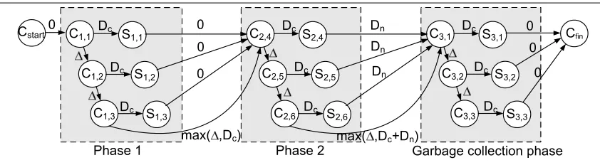
Figure 8: PERT graph of a two-phase update with garbage collection.
Lemma 1. IfU is a multi-phase update procedure, then
the worst-case duration of phasejofUis:
(Nj−1)·∆ +Dc (1)
The following lemma specifies the worst-case update dura-tion of ak-phase update. The intuition is straightforward from Fig. 7.
Lemma 2. The worst-case update duration of a k-phase
update procedure is:
k X
j=1
(Nj−1)·∆ + (k−1)·max(∆, Dc) +Dc (2)
Specifically, intwo-phaseupdatesk= 2, yielding:
Corollary 1. IfUis atwo-phaseupdate procedure, then its worst-case update duration is:
(N1+N2−2)·∆ + max(∆, Dc) +Dc (3)
5.2.2
Untimed Updates with Garbage Collection
In some cases, garbage collection is required for some of the phases in the update procedure. For example, in the two-phase approach, after phase 2 is completed and all en-route packets have been drained from the network, garbage collection is required for theN1 switches of the first phase.
More generally, assume that at the end of every phase j the controller performs garbage collection for a set ofNGj switches. Thus, after phase j is completed the controller waitsDn time units for the en-route packets to drain, and then invokes the garbage collection procedure for theNGj switches.
After invoking the last message of phase j, the controller waits for max(∆, Dc+Dn) time units. Thus, the worst-case duration from the transmission of the last message of phasej until the garbage collection of phasejis completed is given by Eq. 4.
max(∆, Dc+Dn) + (NGj−1)·∆ +Dc (4)
Fig. 8 depicts a PERT graph of a two-phase update pro-cedure that includes a garbage collection phase. At the end of the second phase, garbage collection is performed for the phase 1 policy rules of S1, S2, and S3. This is in
fact a special case of a 3-phase update procedure, where the third phase takes place only after all the en-route pack-ets are guaranteed to have been drained from the network. The main difference between this example and the general k-phase graph of Fig. 7 is that in Fig. 8 the controller waits at leastmax(∆, Dc+Dn) time units from the transmission of the last message of phase 2 until starting to invoke the garbage collection phase.
Lemma 3. If U is a two-phase update procedure with a
garbage collection phase, then its worst-case update duration is:
(N1+N2+NG1−3)·∆ + max(∆, Dc)+ + max(∆, Dc+Dn) +Dc
(5)
5.3
Worst-case Analysis of Timed Updates
5.3.1
Worst-case-based Scheduling
Based on a worst-case analysis, an SDN program can de-termine an update schedule, T= (T1, . . . , Tk, Tg1, . . . , Tg k). Every timed updateut is performed no later than att+δ. Consequently, we can derive the worst-case scheduling con-straints below.
Definition 1 (Worst-case scheduling). If U is a
timed k-phase update procedure, a schedule T =
(T1, . . . , Tk, Tg1, . . . , Tg k)is said to be a worst-case schedule if it satisfies the following two equations:
Tj=Tj−1+δ f or every phase 2≤j≤k (6)
Tg j =Tj+δ+Dn (7) for every phasejthat requires garbage collection
Note that agreedy timed update procedure usesworst-case scheduling.
Cfin
T
g1S
3,1S
3,2S
3,3δ
δ
δ
Garbage collection phase
C
startT
suδ
S
1,1S
1,2S
1,3T
2S
2,4S
2,5S
2,6T
1δ
δ
δ
δ
δ
Phase 1
Phase 2
D
nD
nD
n0
0
0
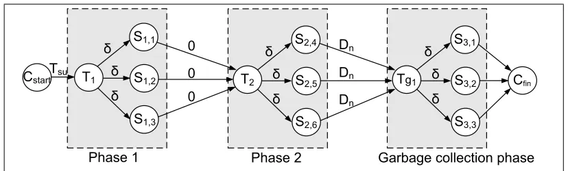
Figure 9: PERT graph of a timed two-phase update with garbage collection.
5.3.2
Timed Updates
A timed update starts with the controller sending scheduled update messages to all the switches, requiring a setup time Tsu. Every phase is guaranteed to take no longer thanδ. An example of a timedtwo-phaseupdate is illustrated in Fig. 9.
Lemma 4. The worst-case update duration of a k-phase
timed update procedure with a worst-case schedule isk·δ.
Based on the latter, we derive the following lemma.
Lemma 5. If U is a two-phase timed update procedure
with a garbage collection phase using a worst-case schedule, then its worst-case update duration isDn+ 3·δ.
5.4
Timed vs. Untimed Updates
We now study the conditions under which the timed ap-proach outperforms the untimed apap-proach.
Based on Lemmas 2 and 4, we observe that a timedk-phase update procedure has a shorter update duration than a sim-ilar untimedk-phase update procedure if:
k·δ <
k X
j=1
(Nj−1)·∆ + (k−1)·max(∆, Dc) +Dc (8)
Lemma 6. LetUT be a greedy timedk-phase update pro-cedure, with a worst-case update duration D1. Let U be a greedy untimed k-phase update procedure with a worst-case update durationD2. Ifδ < Dc andUT ∼U, thenD1< D2.
Now, based on Lemma 3 and Lemma 5, we observe that a timedtwo-phase update procedure with garbage collection has a shorter update duration than a similar untimed two-phaseupdate procedure if:
Dn+ 3·δ <(N1+N2+NG1−3)·∆+
+ max(∆, Dc) + max(∆, Dc+Dn) +Dc
(9)
Lemma 7. Let UT be a greedy timed two-phase update
procedure with a garbage collection phase, with a worst-case
update duration D1. Let Ube a greedy untimed two-phase update procedure with a worst-case update duration D2. If
δ < DcandUT∼U, thenD1< D2.
We have shown that ifδ < Dc the timed approach yields a shorter update duration than the untimed approach, and is thus more scalable. Based on Observation 1, even if switches are not designed for real-time performance we haveδ < Dc. We conclude that the timed approach is the superior one in typical settings.
6.
TIME AS A CONSISTENCY KNOB
6.1
An Inconsistency Metric
As discussed in Section 4, the upper boundsDc andDndo not necessarily exist, or may be very high. Thus, in prac-tice consistent network updates only guarantee consistent forwarding with a high probability, raising the need for a way to measure and quantify to what extent an update is consistent.
Definition 2 (Test flow). A set of packet instances
PI is said to be a test flowif for every two packet instances (pk1, S1, p1, t1)∈PIand(pk2, S2, p2, t2)∈PI, all the follow-ing conditions are satisfied:
• S1=S2. • p1=p2. • pk1=pk2.6
• Packet instances are received at a constant packet ar-rival rateR, i.e., if botht2> t1 and there is no packet
instance (pk3, S3, p3, t3) ∈PI such that t2 > t3 > t1,
thent2=t1+ 1/R.
We assume a method that, for a given test flow f and an updateu, allows to measure the number of packetsn(f, u) that are forwarded inconsistently.7
6
For simplicity, we define that all packets of a test flow are identical. It is in fact sufficient to require that all packets of the flow are indistinguishable by the switch forwarding functions, for example, that all packets of a flow have the same source and destination addresses.
7This measurement can be performed, for example, by
Definition 3 (Inconsistency metric). Letfbe a test flow with a packet arrival rate R(f). Let U be an update, and letn(f, U) be the number of packet instances off that are forwarded inconsistently due to update U. The incon-sistency I(f, U) of a flow f with respect toU is defined to be:
I(f, U) = n(f, U)
R(f) (10)
The inconsistencyI(f, U) is measured in time units. Intu-itively,I(f, U) quantifies the amount of time that flowf is disrupted by the update.
6.2
Fine Tuning Consistency
Timed updates provide a powerful mechanism that allows SDN programmers to tune the degree of consistency. By setting the update times T1, T2, . . . , Tk, Tg1, . . . , Tg k, the controller can play with the consistency-scalability trade-off; the update overhead can be reduced at the expense of some inconsistency, or vice versa.8
Example 1. We consider atwo-phaseupdate with a garbage
collection phase. We assume thatδ= 0and that all packet instances are subject to a constant network delay, Dn. By assigning T = T1 = T2 = Tg1, the controller schedules a
simultaneous update. This approach is referred to as Time-Conf in [29]. All switches are scheduled to perform the update at the same time T. Packets entering the network during the period[T−Dn, T]are forwarded inconsistently. The inconsistency metric in this example is I = Dn. The advantage of this approach is that it completely relieves the switches from the overhead of maintaining duplicate entries between the phases of the update procedure.
Example 2. Again, we consider a two-phase update
(Fig. 10), with δ = 0 and a constant network delay, Dn. We assignT2 =T1+δ according to Eq. 6, andTg1 is
as-signed to be T2+δ+d, whered < Dn. The update is il-lustrated in the PERT graph of Fig. 10. Hence, packets en-tering the network during the period[T2−Dn+d, T2] are
forwarded inconsistently. The inconsistency metric is equal toI=min(Dn−d,0). In a precise sense, the delay dis a knob for tuning the update inconsistency.
7.
EVALUATION
Our evaluation was performed on a 50-node testbed in the DeterLab [44, 28] environment. The nodes (servers) in the DeterLab testbed are interconnected by a user-configurable topology.
Each testbed node in our experiments ran a software-based OpenFlow switch that supports time-based updates, also known asScheduled Bundles [41]. A separate machine was
8
In some scenarios, such as security policy updates, even a small level of inconsistency cannot be tolerated. In other cases, such as path updates, a brief period of inconsistency comes at the cost of some packets being dropped, which can be a small price to pay for reducing the update duration.
Cfin
Tg1
S3,1
S3,2
S3,3
Garbage collection phase
Cstart
Tsu
δ=0 S1,1
S1,2
S1,3 T2
S2,4
S2,5
S2,6
T1 δ=0
Phase 1 Phase 2
d d d 0
0
0 δ=0
δ=0
δ=0
δ=0
δ=0
δ=0
δ=0
Figure 10: Example 2: PERT graph of a timed two-phase update. The delayd(red in the figure) is a knob for consistency.
used as a controller, which was connected to the switches using an out-of-band control network.
The OpenFlow switches and controller we used are a version of OFSoftSwitch and Dpctl [3], respectively, that supports Scheduled Bundles [33]. We used ReversePTP[31, 32] to guarantee synchronized timing.
7.1
Experiment 1: Timed vs. Untimed
Updates
We emulated a typical leaf-spine topology (e.g., [9]) of N switches, with 2N
3 leaf switches, and N
3 spine switches. The
experiments were run using various values ofN, between 6 and 48 switches.
2N/3 leaf
switches
N/3 spine
switches
Figure 13: Leaf-spine topology.
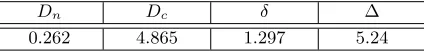
We measured the delay upper bounds, Dn, Dc, δ, and ∆. Table 3 presents the 99.9thpercentile delay values of each of these parameters. These are the parameters that were used in the controller’s greedy updates.
Dn Dc δ ∆
0.262 4.865 1.297 5.24
Table 3: The measured 99.9thpercentile of each of the delay attributes in milliseconds.
We observed a low network delay Dn, as it was measured over two hops of a local area network. In Experiment 2 we analyze networks with a high network delay. Note that the values ofδ and Dc were measured over software-based switches. Since hardware switches may yield different val-ues, some of our experiments were performed with various synthesized values of δ and Dc, as discussed below. The measured value of ∆ was high, on the order of 5 millisec-onds, as Dpctl is not optimized for performance.
(a) Sprint topology. (b) NetRail topology. (c) Compuserve topology.
Figure 11: Publicly available network topologies [7] used in our experiments. Each node in the graph represents an OpenFlow switch.
source destination
(a) Sprint topology.
source
destination
(b) NetRail topology.
source destination
(c) Compuserve topology.
Figure 12: Test flows: each path of the test flows in our experiment is depicted by a different color. Black nodes are OpenFlow switches. White nodes represent the external source and destination of the test flows in the experiment.
(ii) a phase 2 update, involving only the leaf (ingress) switches, and (iii) a garbage collection phase, involving all the switches.
Results. Fig. 14a compares the update duration of the timed and untimed approaches as a function ofN. Untimed updates yield a significantly higher update duration, since they are affected by (N1+N2+NG1−3)·∆, per Lemma 3.9
Hence,the advantage of the timed approach increases with the number of switchesin the network, illustrating its scalability.
9
The slope of the untimed curve in Fig. 14a is ∆, by Lemma 3. The theoretical curve was computed based on the 99.9th percentile value, whereas the mean value in our experiment was about 20% lower, explaining the different slopes of the theoretical and experimental curves.
0 0.1 0.2 0.3 0.4 0.5 0.6 0.7 0.8 0.9
0 10 20 30 40 50
U
p
d
a
te
D
u
ra
ti
o
n
[
se
co
n
d
s]
Number of Switches Timed - experimental Untimed - experimental Timed - theoretical Untimed - theoretical
(a) The update duration as a function of the number of
switches.
0 0.5 1 1.5 2 2.5 3 3.5 4 4.5
-0.2 0 0.2 0.4 0.6 0.8 1
U
p
d
a
te
D
u
ra
ti
o
n
[
se
co
n
d
s]
Dc-δ [seconds] Timed - experimental Untimed - experimental Timed - theoretical Untimed - theoretical
(b) The update duration as a function ofDc−δ, forN= 12, δ= 100 ms, various values ofDc.
Figure 14: Timed updates vs. untimed updates. Each figure shows the experimental values, and the theoretical worst-case values, based on Lemmas 3 and 5.
Fig. 14b shows the update duration of the two approaches as a function ofDc−δ, as we ran the experiment with synthe-sized values ofδandDc. We fixedδat 100 milliseconds, and tested various values ofDc. As expected (by Section 5.4), the results show that for Dc−δ >0 the timed approach yields a lower update duration. Furthermore, only when the scheduling error,δ, is significantly higher thanDcdoes the untimed approach yield a shorter update duration. As discussed in Section 4.3, we typically expect Dc−δ to be positive, asδis unaffected by high network delays, and thus we expect the timed approach to prevail. Interestingly, the results show thateven when the scheduling is not ac-curate, e.g., if δ is 100 milliseconds worse than Dc, the
timed approach has a lower update duration.
7.2
Experiment 2: Fine Tuning Consistency
The goal of this experiment was to study how time can be used to tune the level of inconsistency during updates. In or-der to experiment with real-life wide area network delay val-ues,Dn, we performed the experiment using publicly avail-able topologies.
Network topology. Our experiments ran over three pub-licly available service provider network topologies [7], as il-lustrated in Fig. 11. We defined each node in the figure to be an OpenFlow switch. OpenFlow messages were sent to the switches by a controller over an out-of-band network (not shown in the figures).
recom-0 5 10 15 20 25 30
0 10 20 30
In co n si st en c y [ m il li se co n d s]
Update Duration [milliseconds] flow 1a
flow 2a
flow 3a
flow 4a
flow 5a
(a) Sprint - constant network delay.
0 5 10 15 20 25 30
0 10 20 30
In co n si st en cy [ m il li se co n d s]
Update Duration [milliseconds]
flow 1b flow 2b flow 3b flow 4b flow 5b
(b) NetRail - constant network delay.
0 5 10 15 20 25 30
0 10 20 30
In co n si st en cy [ m il li se co n d s]
Update Duration [milliseconds] flow 1c flow 2c flow 3c flow 4c flow 5c
(c) Compuserve - constant network delay.
0 5 10 15 20 25 30
0 50 100
In co n si st en cy [ m il li se co n d s]
Update Duration [milliseconds] flow 1a
flow 2a
flow 3a
flow 4a
flow 5a
(d) Sprint - exponential network delay.
0 5 10 15 20 25 30
0 50 100
In co n si st e n cy [ m il li se co n d s]
Update Duration [milliseconds]
flow 1b flow 2b flow 3b flow 4b flow 5b
(e) NetRail - exponential network delay.
0 5 10 15 20 25 30
0 20 40 60 80 100
In co n si st en cy [ m il li se co n d s]
Update Duration [milliseconds]
flow 1c flow 2c flow 3c flow 4c flow 5c
(f) Compuserve - exponential network delay.
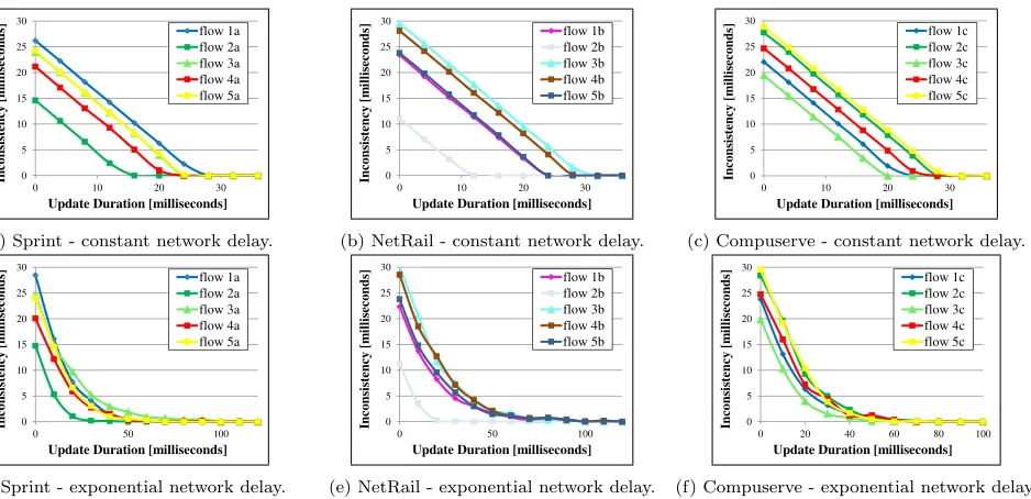
Figure 15: Inconsistency as a function of the update duration. Modifying the update duration controls the degree of incon-sistency. Two graphs are shown for each of the three topologies: exponential delay, constant delay.
mended in [17]. The DeterLab testbed allows a configurable delay value to be assigned to each link. We ran our experi-ments in two modes:
(i)Constant delay — each link had a constant delay that was configured to the value we computed as described above.
(ii) Exponential delay — each link had an exponentially distributed delay. The mean delay of each link in experiment (ii) was equal to the link delay of this link in experiment (i), allowing an ‘apples to apples’ comparison.
Test flows. In each topology we ran five test flows, and measured the inconsistency during a timed network update. Each test flow was injected by an external source (see 12) to one of the ingress switches, forwarded through the network, and transmitted from an egress switch to an external desti-nation. Test flows were injected at a fixed rate of 40 Mbps using Iperf [5].
Network updates. We performed two-phase updates of a Multiprotocol Label Switching (MPLS) label; a flow is forwarded over an MPLS Label-Switched Path (LSP) with label A, and then reconfigured to use label B. A garbage collection phase was used to remove the entries of label A. Conveniently, the MPLS label was also used as the version tag in thetwo-phase updates.
Inconsistency measurement. For every test flowf, and updateU, we measure the number of inconsistent packets during the updaten(f, U). Inconsistent packets in our con-text are either packets with a ‘new’ label arriving to a switch without the ‘new’ rule, or packets with an ‘old’ label arriv-ing to a switch without the ‘old’ configuration. We used the switches’ OpenFlow counters to count the number of incon-sistent packets,n(f, U). We compute the inconsistency of each update using Eq. 10.
Results. We measured the inconsistencyIduring each up-date as a function of the upup-date duration, Tg1−T1. We
repeated the experiment for each of the topologies and each of the test flows of Fig. 12.
The results are illustrated in Fig. 15. The figure depicts the tradeoff between the update duration, and the inconsistency during the update. A long update duration bares a cost on the switches’ expensive memory resources, whereas a high degree of inconsistency implies a large number of dropped or misrouted packets.
Using a timed update, it is possible to tune the difference Tg1−T1, directly affecting the degree of inconsistency. An
SDN programmer can tuneTg1−T1to the desired sweet spot
based on the system constraints; if switch memory resources are scarce, one may reduce the update duration and allow some inconsistency.
As illustrated in Fig. 15d, 15e, and 15f, this fine tuning is especially useful when the network latency has a long-tailed distribution. A truly consistent update, whereI= 0, requires a very long and costly update duration. As shown in the figures, by slightly compromisingI, the switch memory overhead during the update can be cut in half.
8.
DISCUSSION
guaranteeing anall-or-none behavior.
Explicit acknowledgment. As discussed in Section 4.1, OpenFlow currently does not support an explicit acknowl-edgment (ACK) mechanism. In the absence of ACKs, up-date procedures are planned according to aworst-case anal-ysis (Section 5), both in the timed and in the untimed ap-proaches. However, if switches are able to notify the con-troller upon completion of an update (as assumed in [18]), then update procedures can sometimes be completed ear-lier than without using ACKs. Furthermore, ACKs enable updates to be performed dynamically [18], whereby at the end of each phase the controller dynamically plans the next phase. Fortunately, the timed and untimed approaches can be combined. For example, in the presence of an acknowl-edgment mechanism, update procedures can be performed in a dynamic, untimed, ACK-based manner, with a timed garbage collection phase at the end. This flexible mix-and-match approach allows the SDN programmer to enjoy the best of both worlds.
9.
RELATED WORK
The use of time in distributed applications has been widely analyzed, both in theory and in practice. Analysis of the us-age of time and synchronized clocks, e.g., Lamport [21, 22] dates back to the late 1970s and early 1980s. Accurate time has been used in various different applications, such as dis-tributed database [10], industrial automation systems [14], automotive networks [15], and accurate instrumentation and measurements [36]. While the usage of accurate time in dis-tributed systems has been widely discussed in the literature, we are not aware of similar analyses of the usage of accu-rate time as a means for performing consistent updates in computer networks.
Time-of-day routing [8] routes traffic to different destina-tions based on the time-of-day. Path calendaring [19] can be used to configure network paths based on scheduled or foreseen traffic changes. The two latter examples are typi-cally performed at a low rate and do not place demanding requirements on accuracy.
In [12] the authors briefly mentioned that it would be in-teresting to explore using time synchronization to instruct routers or switches to change from one configuration to an-other at a specific time, but did not pursue the idea beyond this observation. Our previous work [29, 30] introduced the concept of using time to coordinate updates in SDN. Based on our work [33], the OpenFlow protocol [41, 40] currently supports time-based network updates. In [34] we presented a practical method to implement accurately scheduled net-work updates. In this paper we analyze the use of time inconsistent updates, and show that time can improve the scalability of consistent updates.
Various consistent network update approaches have been an-alyzed in the literature. Two of the most well-known update methods are the ordered approach [11, 45, 24, 18], and the two-phase approach [42, 20]. None of these works proposed to use accurate time and synchronized clocks as a means to coordinate the updates. In this paper we show that time can be used to improve these two methods, allowing to reduce the overhead during update procedures.
The analysis of [20] proposed an incremental method that improves the scalability of consistent updates by breaking each update into multiple independent rounds, thereby re-ducing the total overhead consumed in each separate round. The timed approach we present in this paper can improve the incremental method even further, by reducing the over-head consumed in each round.
10.
CONCLUSION
Accurate time synchronization has become a common fea-ture in commodity switches and routers. We have shown that it can be used to implement consistent updates in a way that reduces the update duration and the expensive over-head of maintaining duplicate configurations. Moreover, we have shown that accurate time can be used to tune the fine tradeoff between consistency and scalability during network updates. Our experimental evaluation demonstrates that timed updates allow scalability that would not be possible with conventional update methods.
Acknowledgments
This work was supported in part by the ISF grant 1520/11. We gratefully acknowledge the DeterLab project [44] for the opportunity to perform our experiments on the DeterLab testbed.
A.
APPENDIX: DATASET DETAILS
The measurement results presented in Section 4.1 are based on publicly available datasets from [6, 2]. The data we an-alyzed consists of RTT measurements between 20 source-destination pairs, listed in Table 4. The data is based on measurements taken from November 2013 to November 2014.
Source site Destination site Trace source
ping.desy.de ba.sanet.sk [6]
pinger.stanford.edu ihep.ac.cn [6]
pinger.stanford.edu institutokilpatrick .edu
[6]
pinger.uet.edu.pk ping.cern.ch [6] pinger2.if.ufrj.br ping.cern.ch [6] pinger.arn.dz dns.sinica.edu.tw [6] pinger.stanford.edu ping.cern.ch [6] pinger.stanford.edu mail.gnet.tn [6] pinger.stanford.edu tg.refer.org [6] pinger.stanford.edu www.unitec.edu [6]
ampz-catalyst ampz-citylink [2]
ampz-inspire ampz-massey-pn [2]
ampz-netspace ampz-inspire [2]
ampz-ns3a ampz-citylink [2]
ampz-ns3a www.stuff.co.nz [2]
ampz-rurallink www.facebook.com [2] ampz-rurallink www.google.co.nz [2] ampz-waikato www.facebook.com [2] ampz-waikato www.google.co.nz [2]
ampz-wxc-akl ampz-csotago [2]
11.
REFERENCES
[1] Connectivity Fault Management.IEEE Std 802.1ag, 2007.
[2] AMP Measurements.http://erg.wand.net.nz, 2014. [3] CPqD OFSoftswitch.
https://github.com/CPqD/ofsoftswitch13, 2014. [4] IEEE 1588 time synchronization deployment for
mobile backhaul in China Mobile. keynote presentation, International IEEE Symposium on Precision Clock Synchronization for Measurement Control and Communication (ISPCS), 2014.
[5] Iperf - The TCP/UDP Bandwidth Measurement Tool. https://iperf.fr/, 2014.
[6] PingER.http://pinger.fnal.gov/, 2014. [7] Topology Zoo.http://topology-zoo.org/, 2015. [8] G. R. Ash. Use of a trunk status map for real-time
DNHR. InInternational TeleTraffic Congress (ITC-11), 1985.
[9] Cisco. Cisco’s Massively Scalable Data Center.http: //www.cisco.com/c/dam/en/us/td/docs/solutions/ Enterprise/Data_Center/MSDC/1-0/MSDC_AAG_1.pdf, 2010.
[10] J. C. Corbett et al. Spanner: Google’s
globally-distributed database. InOSDI, volume 1, 2012.
[11] P. Francois and O. Bonaventure. Avoiding transient loops during the convergence of link-state routing protocols.IEEE/ACM Transactions on Networking, 15(6):1280–1292, 2007.
[12] A. Greenberg, G. Hjalmtysson, D. A. Maltz, A. Myers, J. Rexford, G. Xie, H. Yan, J. Zhan, and H. Zhang. A clean slate 4D approach to network control and management.ACM SIGCOMM Computer Communication Review, 35(5):41–54, 2005. [13] O. Gurewitz, I. Cidon, and M. Sidi. One-way delay
estimation using network-wide measurements. IEEE/ACM Transactions on Networking (TON), 14(SI):2710–2724, 2006.
[14] K. Harris. An application of IEEE 1588 to industrial automation. InInternational IEEE Symposium on Precision Clock Synchronization for Measurement Control and Communication (ISPCS), 2008. [15] IEEE. Time-Sensitive Networking Task Group.
http://www.ieee802.org/1/pages/tsn.html, 2012. [16] IEEE TC 9. 1588 IEEE Standard for a Precision Clock
Synchronization Protocol for Networked Measurement and Control Systems Version 2.IEEE, 2008.
[17] ITU-T G.144. One-way transmission time.ITU-T, 2003.
[18] X. Jin, H. H. Liu, R. Gandhi, S. Kandula, R. Mahajan, J. Rexford, R. Wattenhofer, and M. Zhang. Dionysus: Dynamic scheduling of network updates. InACM SIGCOMM, 2014.
[19] S. Kandula, I. Menache, R. Schwartz, and S. R. Babbula. Calendaring for wide area networks. InACM SIGCOMM, 2014.
[20] N. P. Katta, J. Rexford, and D. Walker. Incremental consistent updates. InACM SIGCOMM workshop on Hot topics in Software Defined Networks (HotSDN), 2013.
[21] L. Lamport. Time, clocks, and the ordering of events
in a distributed system.Communications of the ACM, 21(7):558–565, 1978.
[22] L. Lamport. Using time instead of timeout for fault-tolerant distributed systems.ACM Trans. Program. Lang. Syst., 6(2):254–280, Apr. 1984. [23] L. Lamport and P. M. Melliar-Smith. Synchronizing
clocks in the presence of faults.Journal of the ACM (JACM), 32(1):52–78, 1985.
[24] H. H. Liu, X. Wu, M. Zhang, L. Yuan,
R. Wattenhofer, and D. Maltz. zUpdate: updating data center networks with zero loss. InACM SIGCOMM. ACM, 2013.
[25] D. G. Malcolm, J. H. Roseboom, C. E. Clark, and W. Fazar. Application of a technique for research and development program evaluation.Operations research, 7(5):646–669, 1959.
[26] N. McKeown, T. Anderson, H. Balakrishnan, G. Parulkar, L. Peterson, J. Rexford, S. Shenker, and J. Turner. Openflow: enabling innovation in campus networks.ACM SIGCOMM Computer
Communication Review, 38(2):69–74, Mar. 2008. [27] Metro Ethernet Forum. Ethernet services attributes
-phase 3.MEF 10.3, 2013.
[28] J. Mirkovic and T. Benzel. Teaching cybersecurity with DeterLab.Security & Privacy, IEEE, 10(1):73–76, 2012.
[29] T. Mizrahi and Y. Moses. Time-based updates in software defined networks. InACM SIGCOMM workshop on Hot topics in Software Defined Networks (HotSDN), 2013.
[30] T. Mizrahi and Y. Moses. On the necessity of time-based updates in SDN. InOpen Networking Summit (ONS), 2014.
[31] T. Mizrahi and Y. Moses.ReversePTP: A software defined networking approach to clock synchronization. InACM SIGCOMM workshop on Hot topics in Software Defined Networks (HotSDN), 2014. [32] T. Mizrahi and Y. Moses. UsingReversePTPto
distribute time in software defined networks. In International IEEE Symposium on Precision Clock Synchronization for Measurement Control and Communication (ISPCS), 2014.
[33] T. Mizrahi and Y. Moses.Time4: Time for SDN. technical report, arXiv preprint arXiv:1505.03421, 2015.
[34] T. Mizrahi, O. Rottenstreich, and Y. Moses. TimeFlip: Scheduling network updates with timestamp-based TCAM ranges. InIEEE INFOCOM, 2015.
[35] T. Mizrahi, E. Saat, and Y. Moses. Timed consistent network updates. technical report, arXiv preprint arXiv:1505.03653, 2015.
[36] P. Moreira et al. White rabbit: Sub-nanosecond timing distribution over ethernet. InInternational IEEE Symposium on Precision Clock Synchronization for Measurement Control and Communication (ISPCS), 2009.
[37] A. Mukherjee. On the dynamics and significance of low frequency components of internet load.Technical Reports (CIS), page 300, 1992.
paper,http://www.networktest.com/, 2010. [39] Open Networking Foundation. Openflow switch
specification.Version 1.4.0, 2013.
[40] Open Networking Foundation. Openflow extensions 1.3.x package 2. 2015.
[41] Open Networking Foundation. Openflow switch specification.Version 1.5.0, 2015.
[42] M. Reitblatt, N. Foster, J. Rexford, C. Schlesinger, and D. Walker. Abstractions for network update. In ACM SIGCOMM, 2012.
[43] C. Rotsos, N. Sarrar, S. Uhlig, R. Sherwood, and A. W. Moore. Oflops: An open framework for openflow switch evaluation. InPassive and Active Measurement, pages 85–95. Springer, 2012. [44] The DeterLab project.
http://deter-project.org/about_deterlab, 2015. [45] L. Vanbever, S. Vissicchio, C. Pelsser, P. Francois, and
O. Bonaventure. Seamless network-wide igp migrations. InACM SIGCOMM Computer
![Figure 11: Publicly available network topologies [7] used in our experiments. Each node in the graph represents an OpenFlowswitch.](https://thumb-us.123doks.com/thumbv2/123dok_us/345402.2031524/10.612.62.548.51.165/figure-publicly-available-network-topologies-experiments-represents-openflowswitch.webp)