Vacuum Fundamentals Lybold

(1)

00.200.02

Kat.-Nr. 199 90

Fundamentals of

(2)

Preface

Oerlikon Leybold Vacuum, a member of the globally active industrial Oerlikon Group of companies has developed into the world market leader in the area of vacuum technology. In this leading position, we recognize that our customers around the world count on Oerlikon Leybold Vacuum to deliver technical superiority and maximum value for all our products and services. Today, Oerlikon Leybold Vacuum is strengthening that well-deserved reputation by offering a wide array of vacuum pumps and aftermarket services to meet your needs.

This brochure is meant to provide an easy to read overview covering the entire range of vacuum technology and is inde-pendent of the current Oerlikon Leybold Vacuum product portfolio. The presented product diagrams and data are pro-vided to help promote a more comprehensive understanding of vacuum technology and are not offered as an implied war-ranty. Content has been enhanced through the addition of new topic areas with an emphasis on physical principles affecting vacuum technology.

To us, partnership-like customer relationships are a funda-mental component of our corporate culture as well as the continued investments we are making in research and development for our next generation of innovative vacuum technology products. In the course of our over 150 year-long corporate history, Oerlikon Leybold Vacuum developed a comprehensive understanding of process and application know-how in the field of vacuum technology. Jointly with our partner customers, we plan to continue our efforts to open up further markets, implement new ideas and develop pioneer-ing products.

(3)

(4)

Preface

Fundamentals

of Vacuum

Technology

revised and compiled by

Dr. Walter Umrath

with contributions from

(5)

(6)

Table of Contents

2.2 Choice of pumping process . . . .60

2.2.1 Survey of the most usual pumping processes . . . .60

2.2.2 Pumping of gases (dry processes) . . . .62

2.2.3 Pumping of gases and vapors (wet processes) . . . .62

2.2.4 Drying processes . . . .64

2.2.5 Production of an oil-free (hydrocarbon-free) vacuum . . . .65

2.2.6 Ultrahigh vacuum working Techniques . . . .65

2.3 Evacuation of a vacuum chamber and determination of pump sizes . . . .66

2.3.1 Evacuation of a vacuum chamber (without additional sources of gas or vapor) . . . .66

2.3.1.1 Evacuation of a chamber in the rough vacuum region . . . .67

2.3.1.2 Evacuation of a chamber in the high vacuum region . . . .68

2.3.1.3 Evacuation of a chamber in the medium vacuum region . . . . .68

2.3.2 Determination of a suitable backing pump . . . .69

2.3.3 Determination of pump-down time from nomograms . . . .70

2.3.4 Evacuation of a chamber where gases and vapors are evolved . . . .71

2.3.5 Selection of pumps for drying processes . . . .71

2.3.6 Flanges and their seals . . . .73

2.3.7 Choice of suitable valves . . . .73

2.3.8 Gas locks and seal-off fittings . . . .75

3. Vacuum measurement, monitoring, control and regulation . . . .76

3.1 Fundamentals of low-pressure measurement . . . .76

3.2 Vacuum gauges with pressure reading that is independent of the type of gas . . . .77

3.2.1 Bourdon vacuum gauges . . . .77

3.2.2 Diaphragm vacuum gauges . . . .77

3.2.2.1 Capsule vacuum gauges . . . .77

3.2.2.2 DIAVAC diaphragm vacuum gauge . . . .78

3.2.2.3 Precision diaphragm vacuum gauges . . . .78

3.2.2.4 Capacitance diaphragm gauges . . . .78

3.2.3 Liquid-filled (mercury) vacuum gauges . . . .79

3.2.3.1 U-tube vacuum gauges . . . .79

3.2.3.2 Compression vacuum gauges (according to McLeod) . . . .79

3.3 Vacuum gauges with gas-dependent pressure reading . . . .81

3.3.1 Spinning rotor gauge (SRG) (VISCOVAC) . . . .81

3.3.2 Thermal conductivity vacuum gauges . . . .82

3.3.3 Ionization vacuum gauges . . . .83

3.3.3.1 Cold-cathode ionization vacuum gauges (Penning vacuum gauges) . . . .83

3.3.3.2 Hot-cathode ionization vacuum gauges . . . .84

3.4 Adjustment and calibration; DKD, PTB national standards . . . .86

3.4.1 Examples of fundamental pressure measurement methods (as standard methods for calibrating vacuum gauges . . . .87

3.5 Pressure monitoring,control and regulation in vacuum systems . . . .88

3.5.1 Fundamentals of pressure monitoring and control . . . .88

3.5.2 Automatic protection, monitoring and control of vacuum systems . . . .89

3.5.3 Pressure regulation and control in rough and medium vacuum systems . . . .90

3.5.4 Pressure regulation in high and ultrahigh vacuum systems . . .92

3.5.5 Examples of applications with diaphragm controllers . . . .93

1. Vacuum physics Quantities, their symbols, units of measure and definitions . . . .9

1.1 Basic terms and concepts in vacuum technology . . . .9

1.2 Atmospheric air . . . .13

1.3 Gas laws and models . . . .13

1.3.1 Continuum theory . . . .13

1.3.2 Kinetic gas theory . . . .13

1.4 The pressure ranges in vacuum technology and their characterization . . . 14

1.5 Types of flow and conductance . . . .15

1.5.1 Types of flow . . . .15

1.5.2 Calculating conductance values . . . .16

1.5.3 Conductance for piping and openings . . . .16

1.5.4 Conductance values for other elements . . . .18

2. Vacuum Generation . . . .19

2.1 Vacuum pumps: A survey . . . .19

2.1.1 Oscillation displacement vacuum pumps . . . .20

2.1.1.1 Diaphragm pumps . . . .20

2.1.2 Liquid sealed rotary displacement pumps . . . .20

2.1.2.1 Liquid ring pumps . . . .20

2.1.2.2 Oil sealed rotary displacement pumps . . . .21

2.1.2.2.1 Rotary vane pumps (TRIVAC A, TRIVAC B, TRIVAC E, SOGEVAC) . . . .21

2.1.2.2.2 Rotary plunger pumps (E Pumps) . . . .23

2.1.2.2.3 Trochoid pumps . . . .24

2.1.2.2.4 The gas ballast . . . .24

2.1.3 Dry compressing rotary displacement pumps . . . .27

2.1.3.1 Roots pumps . . . .27

2.1.3.2 Claw pumps . . . .31

2.1.3.2.1 Claw pumps with internal compression for the semiconductor industry (“DRYVAC Series”) . . . .33

2.1.3.2.2 Claw pump without internal compression for chemistry applications (“ALL·ex”) . . . .35

2.1.4 Accessories for oil-sealed rotary displacement pumps . . . .38

2.1.5 Condensers . . . .38

2.1.6 Fluid-entrainment pumps . . . .40

2.1.6.1 (Oil) Diffusion pumps . . . .41

2.1.6.2 Oil vapor ejector pumps . . . .43

2.1.6.3 Pump fluids . . . .44

2.1.6.4 Pump fluid backstreaming and its suppression (Vapor barriers, baffles) . . . .44

2.1.6.5 Water jet pumps and steam ejectors . . . .45

2.1.7 Turbomolecular pumps . . . .46

2.1.8 Sorption pumps . . . .50

2.1.8.1 Adsorption pumps . . . .50

2.1.8.2 Sublimation pumps . . . .51

2.1.8.3 Sputter-ion pumps . . . .51

2.1.8.4 Non evaporable getter pumps (NEG pumps) . . . .53

2.1.9 Cryopumps . . . .54

2.1.9.1 Types of cryopump . . . .54

2.1.9.2 The cold head and its operating principle . . . .55

2.1.9.3 The refrigerator cryopump . . . .56

2.1.9.4 Bonding of gases to cold surfaces . . . .56

2.1.9.5 Pumping speed and position of the cryopanels . . . .57

(7)

Vacuum physics

1.

Quantities, their symbols, units of measure

and definitions

(cf. DIN 28 400, Part 1, 1990, DIN 1314 and DIN 28 402)

1.1

Basic terms and concepts in vacuum

tech-nology

Pressure p (mbar)

of fluids (gases and liquids). (Quantity: pressure; symbol: p; unit of mea-sure: millibar; abbreviation: mbar.) Pressure is defined in DIN Standard 1314 as the quotient of standardized force applied to a surface and the extent of this surface (force referenced to the surface area). Even though the Torr is no longer used as a unit for measuring pressure (see Section 10), it is nonetheless useful in the interest of “transparency” to mention this pressure unit: 1 Torr is that gas pressure which is able to raise a column of mercury by 1 mm at 0 °C. (Standard atmospheric pressure is 760 Torr or 760 mm Hg.) Pressure p can be more closely defined by way of subscripts:

Absolute pressure pabs

Absolute pressure is always specified in vacuum technology so that the “abs” index can normally be omitted.

Total pressure p_t

The total pressure in a vessel is the sum of the partial pressures for all the gases and vapors within the vessel.

Partial pressure p_i

The partial pressure of a certain gas or vapor is the pressure which that gas or vapor would exert if it alone were present in the vessel.

Important note:Particularly in rough vacuum technology, partial pressure in a mix of gas and vapor is often understood to be the sum of the partial pressures for all the non-condensable components present in the mix – in case of the “partial ultimate pressure” at a rotary vane pump, for example.

Saturation vapor pressure ps

The pressure of the saturated vapor is referred to as saturation vapor pres-sure p_s. p_swill be a function of temperature for any given substance.

Vapor pressure p_d

Partial pressure of those vapors which can be liquefied at the temperature of liquid nitrogen (LN₂).

Standard pressure p_n

Standard pressure p_nis defined in DIN 1343 as a pressure of p_n= 1013.25 mbar.

Ultimate pressure pend

The lowest pressure which can be achieved in a vacuum vessel. The socalled ultimate pressure p_enddepends not only on the pump’s suction speed but also upon the vapor pressure p_dfor the lubricants, sealants and propellants used in the pump. If a container is evacuated simply with an oil-sealed rotary (positive displacement) vacuum pump, then the ultimate pressure which can be attained will be determined primarily by the vapor pressure of the pump oil being used and, depending on the cleanliness of the vessel, also on the vapors released from the vessel walls and, of course, on the leak tightness of the vacuum vessel itself.

Ambient pressure p_amb

or(absolute) atmospheric pressure

Overpressure p_eor gauge pressure

(Index symbol from “excess”) p_e= p_abs– p_amb

Here positive values for p_ewill indicate overpressure or gauge pressure; negative values will characterize a vacuum.

Working pressure pW

During evacuation the gases and/or vapors are removed from a vessel. Gases are understood to be matter in a gaseous state which will not, how-ever, condense at working or operating temperature. Vapor is also matter in a gaseous state but it may be liquefied at prevailing temperatures by increasing pressure. Finally, saturated vapor is matter which at the prevail-ing temperature is gas in equilibrium with the liquid phase of the same sub-stance. A strict differentiation between gases and vapors will be made in the comments which follow only where necessary for complete understanding.

Particle number density n (cm-3₎

According to the kinetic gas theory the number n of the gas molecules, ref-erenced to the volume, is dependent on pressure p and thermodynamic temperature T as expressed in the following:

p = n · k · T (1.1)

n = particle number density k = Boltzmann’s constant

At a certain temperature, therefore, the pressure exerted by a gas depends only on the particle number density and not on the nature of the gas. The nature of a gaseous particle is characterized, among other factors, by its mass m_T.

Gas density ρ(kg · m-3_{, g · cm}-3₎

The product of the particle number density n and the particle mass m_Tis the gas density ρ:

ρ= n · m_T (1.2)

The ideal gas law

The relationship between the mass m_Tof a gas molecule and the molar mass M of this gas is as follows:

(11)

Vacuum physics

Avogadro’s number (or constant) N_Aindicates how many gas particles will be contained in a mole of gas. In addition to this, it is the proportionality factor between the gas constant R and Boltzmann’s constant k:

R = N_A· k (1.4)

Derivable directly from the above equations (1.1) to (1.4) is the correlation between the pressure p and the gas density

ρ

of an ideal gas.

R · T

p

=

ρ

⋅ (1.5)

M

In practice we will often consider a certain enclosed volume V in which the gas is present at a certain pressure p. If m is the mass of the gas present within that volume, then

m

ρ= −−− (1.6)

V

The ideal gas law then follows directly from equation (1.5): m

p⋅ V= −−− ⋅ R⋅ T = ν ⋅ R⋅ T (1.7) M

Here the quotient m / M is the number of moles υpresent in volume V. The simpler form applies for m / M = 1, i.e. for 1 mole:

p · V = R · T (1.7a)

The following numerical example is intended to illustrate the correlation between the mass of the gas and pressure for gases with differing molar masses, drawing here on the numerical values in Table IV (Chapter 9). Contained in a 10-liter volume, at 20 °C, will be

a) 1g of helium b) 1g of nitrogen

When using the equation (1.7) there results then at V = 10 l , m = 1 g,

R = 83.14 mbar · l· mol–1_{· K}–1_{, T = 293 K (20 °C)}

In case a) where M = 4 g · mole-1_{(monatomic gas):} In case b), with M = 28 ≠g mole-1_{(diatomic gas):}

The result, though appearing to be paradoxical, is that a certain mass of a light gas exerts a greater pressure than the same mass of a heavier gas. If one takes into account, however, that at the same gas density (see Equation 1.2) more particles of a lighter gas (large n, small m) will be pre-sent than for the heavier gas (small n, large m), the results become more understandable since only the particle number density n is determinant for the pressure level, assuming equal temperature (see Equation 1.1).

The main task of vacuum technology is to reduce the particle number den-sity n inside a given volume V. At constant temperature this is always equivalent to reducing the gas pressure p. Explicit attention must at this point be drawn to the fact that a reduction in pressure (maintaining the volume) can be achieved not only by reducing the particle number density n but also (in accordance with Equation 1.5) by reducing temperature T at constant gas density. This important phenomenon will always have to be taken into account where the temperature is not uniform throughout volume V.

The following important terms and concepts are often used in vacuum technology:

Volume V (l, m3_{, cm}3₎

The term volume is used to designate

a) the purely geometric, usually predetermined, volumetric content of a vacuum chamber or a complete vacuum system including all the piping and connecting spaces (this volume can be calculated);

b) the pressure-dependent volume of a gas or vapor which, for example, is moved by a pump or absorbed by an adsorption agent.

Volumetric flow (flow volume) qv

(l/s, m3_{/h, cm}3_{/s )}

The term “flow volume” designates the volume of the gas which flows through a piping element within a unit of time, at the pressure and tempera-ture prevailing at the particular moment. Here one must realize that, although volumetric flow may be identical, the number of molecules moved may differ, depending on the pressure and temperature.

Pumping speed S (l/s, m3_{/h, cm}3_{/s )}

The pumping speed is the volumetric flow through the pump’s intake port. dV

S = ₋₋₋ (1.8a)

dt

If S remains constant during the pumping process, then one can use the difference quotient instead of the differential quotient:

ΔV

S = ₋₋₋ (1.8b)

Δt

(A conversion table for the various units of measure used in conjunction with pumping speed is provided in Section 9, Table VI).

Quantity of gas (pV value), (mbar

⋅

l)

The quantity of a gas can be indicated by way of its mass or its weight in the units of measure normally used for mass or weight. In practice, howev-er, the product of p · V is often more interesting in vacuum technology than the mass or weight of a quantity of gas. The value embraces an energy dimension and is specified in millibar · liters (mbar · l) (Equation 1.7). Where the nature of the gas and its temperature are known, it is possible to use Equation 1.7b to calculate the mass m for the quantity of gas on the basis of the product of p · V:

(1.7)

p V m M R T

· = · ·

mbar

=

609

p g mbar mol K K

K g mol

= · · · · ·

·

· · ·

– –

–

1 83 14 293

10 4 1 1 1 . · · · · mbar = = 87

p g mbar mol K K

K g mol

= · · · · ·

·

· · ·

– –

–

1 83 14 293

(12)

Vacuum physics

(1.7b)

Although it is not absolutely correct, reference is often made in practice to the “quantity of gas” p · V for a certain gas. This specification is incomplete; the temperature of the gas T, usually room temperature (293 K), is normally implicitly assumed to be known.

Example:The mass of 100 mbar · l of nitrogen (N₂) at room temperature (approx. 300 K) is:

Analogous to this, at T = 300 K: 1 mbar · l O₂= 1.28 · 10-3_{g O}

2 70 mbar · l Ar = 1.31 · 10-1_{g Ar}

The quantity of gas flowing through a piping element during a unit of time – in accordance with the two concepts for gas quantity described above – can be indicated in either of two ways, these being:

Mass flow q_m(kg/h, g/s),

this is the quantity of a gas which flows through a piping element, referenced to time

m

q_m= ₋₋₋ or as

t

pV flow q_pV(mbar · l · s–1_).

pV flow is the product of the pressure and volume of a quantity of gas flow-ing through a pipflow-ing element, divided by time, i.e.:

p · V d (p · V)

q_pV= _{⎯⎯⎯ = ⎯⎯⎯⎯}

t dt

pV flow is a measure of the mass flow of the gas; the temperature to be indicated here.

Pump throughput qpV

The pumping capacity (throughput) for a pump is equal either to the mass flow through the pump intake port:

m

q_m= ⎯⎯ (1.9)

t

or to the pV flow through the pump’s intake port: p · V

q_pV= ⎯⎯⎯ t

It is normally specified in mbar · l · s–1_{. Here p is the pressure on the intake} side of the pump. If p and V are constant at the intake side of the pump, the throughput of this pump can be expressed with the simple equation

m

mbar

g mol

mbar

mol

K

=

·

· ·

·

−

− −

100

28

83

300

1

1 1

g

=

·

=

2800

300 83

0 113

.

m p V M

R T = · ·

· qpV= p · S (1.10a)

where S is the pumping speed of the pump at intake pressure of p. (The throughput of a pump is often indicated with Q, as well.)

The concept of pump throughput is of major significance in practice and should not be confused with the pumping speed! The pump throughput is the quantity of gas moved by the pump over a unit of time, expressed in mbar≠l/s; the pumping speed is the “transportation capacity” which the pump makes available within a specific unit of time, measured in m3_/h or l/s.

The throughput value is important in determining the size of the backing pump in relationship to the size of a high vacuum pump with which it is con-nected in series in order to ensure that the backing pump will be able to “take off” the gas moved by the high vacuum pump (see Section 2.32).

Conductance C (l · s–1₎

The pV flow through any desired piping element, i.e. pipe or hose, valves, nozzles, openings in a wall between two vessels, etc., is indicated with

q_pV= C(p₁– p₂) = Δp · C (1.11)

Here Δp = (p₁– p₂) is the differential between the pressures at the inlet and outlet ends of the piping element. The proportionality factor C is designated as the conductance value or simply “conductance”. It is affected by the geometry of the piping element and can even be calculated for some sim-pler configurations (see Section 1.5).

In the high and ultrahigh vacuum ranges, C is a constant which is indepen-dent of pressure; in the rough and medium-high regimes it is, by contrast, dependent on pressure. As a consequence, the calculation of C for the pip-ing elements must be carried out separately for the individual pressure ranges (see Section 1.5 for more detailed information).

From the definition of the volumetric flow it is also possible to state that: The conductance value C is the flow volume through a piping element. The equation (1.11) could be thought of as “Ohm’s law for vacuum technology”, in which q_pVcorresponds to current, Δp the voltage and C the electrical conductance value. Analogous to Ohm’s law in the science of electricity, the resistance to flow

1 R= −−−

C

has been introduced as the reciprocal value to the conductance value. The equation (1.11) can then be re-written as:

1

q_pV= —— · Δp (1.12)

R

The following applies directly for connection in series:

R∑= R1 + R2 + R3 . . . (1.13)

When connected in parallel, the following applies:

1 1 1 1

--- _{= −−− + −−− + −−− + ⋅ ⋅ ⋅ ⋅} (1.13a)

(13)

Vacuum physics

Leak rate q_L(mbar · l · s–1₎

According to the definition formulated above it is easy to understand that the size of a gas leak, i.e. movement through undesired passages or “pipe” elements, will also be given in mbar · l · s–1_{. A leak rate is often measured} or indicated with atmospheric pressure prevailing on the one side of the barrier and a vacuum at the other side (p < 1 mbar). If helium (which may be used as a tracer gas, for example) is passed through the leak under exactly these conditions, then one refers to “standard helium conditions”.

Outgassing(mbar · l)

The term outgassing refers to the liberation of gases and vapors from the walls of a vacuum chamber or other components on the inside of a vacuum system. This quantity of gas is also characterized by the product of p · V, where V is the volume of the vessel into which the gases are liberated, and by p, or better Δp, the increase in pressure resulting from the introduction of gases into this volume.

Outgassing rate (mbar · l · s–1₎

This is the outgassing through a period of time, expressed in mbar · l · s–1_.

Outgassing rate (mbar · l · s–1_{· cm}–2₎

(referenced to surface area)

In order to estimate the amount of gas which will have to be extracted, knowledge of the size of the interior surface area, its material and the sur-face characteristics, their outgassing rate referenced to the sursur-face area and their progress through time are important.

Mean free path of the moleculesλ(cm)and collision rate z (s-1₎ The concept that a gas comprises a large number of distinct particles between which – aside from the collisions – there are no effective forces, has led to a number of theoretical considerations which we summarize today under the designation “kinetic theory of gases”.

One of the first and at the same time most beneficial results of this theory was the calculation of gas pressure p as a function of gas density and the mean square of velocity c2_{for the individual gas molecules in the mass of} molecules m_T:

1 __ 1 __

p = --- ρ ⋅ c2_{= ----}⋅ _n⋅ _m

T⋅ c2 (1.14)

3 3

where

__ _k·_T

c2_{= 3}⋅ _--- _(1.15)

m_T

The gas molecules fly about and among each other, at every possible velocity, and bombard both the vessel walls and collide (elastically) with each other. This motion of the gas molecules is described numerically with the assistance of the kinetic theory of gases. A molecule’s average number of collisions over a given period of time, the so-called collision index z, and the mean path distance which each gas molecule covers between two colli-sions with other molecules, the so-called mean free path length λ, are described as shown below as a function of the mean molecule velocity

c-the molecule diameter 2r and c-the particle number density molecules n – as a very good approximation:

---C

Z = --- (1.16)

λ

where (1.17)

and (1.18)

Thus the mean free path length λfor the particle number density n is, in accordance with equation (1.1), inversely proportional to pressure p. Thus the following relationship holds, at constant temperature T, for every gas

λ ⋅p = const (1.19)

Used to calculate the mean free path length λ for any arbitrary pressures and various gases are Table III and Fig. 9.1 in Chapter 9. The equations in gas kinetics which are most important for vacuum technology are also summa-rized (Table IV) in chapter 9.

Impingement rate z_A(cm–2_⋅_s–1_{) and}

monolayer formation time

τ

(s)

A technique frequently used to characterize the pressure state in the high vacuum regime is the calculation of the time required to form a monomole-cular or monoatomic layer on a gas-free surface, on the assumption that every molecule will stick to the surface. This monolayer formation time is closely related with the so-called impingement rate z_A. With a gas at rest the impingement rate will indicate the number of molecules which collide with the surface inside the vacuum vessel per unit of time and surface area:

(1.20)

If a is the number of spaces, per unit of surface area, which can accept a specific gas, then the monolayer formation time is

(1.21)

Collision frequency z_v(cm–3_{· s}–1₎

This is the product of the collision rate z and the halfof the particle number density n, since the collision of twomolecules is to be counted as only one

collision:

(1.21a)

z_V=n·z 2

τ

=

·

a

z

a

n c

A

4

z_A= n c·

4

( )

λ

π

=

·

· ·

1

2

n

2

r

2

c

k T

m

R T

M

T

=

· ·

·

=

· ·

·

8

(14)

Vacuum physics

1.2

Atmospheric air

Prior to evacuation, every vacuum system on earth contains air and it will always be surrounded by air during operation. This makes it necessary to be familiar with the physical and chemical properties of atmospheric air. The atmosphere is made up of a number of gases and, near the earth’s surface, water vapor as well. The pressure exerted by atmospheric air is referenced to sea level. Average atmospheric pressure is 1013 mbar (equivalent to the “atmosphere”, a unit of measure used earlier). Table VIII in Chapter 9 shows the composition of the standard atmosphere at relative humidity of 50 % and temperature of 20 °C. In terms of vacuum technology the following points should be noted in regard to the composition of the air: a) The water vapor contained in the air, varying according to the humidity

level, plays an important part when evacuating a vacuum plant (see Section 2.2.3).

b) The considerable amount of the inert gas argon should be taken into account in evacuation procedures using sorption pumps (see Section 2.1.8).

c) In spite of the very low content of helium in the atmosphere, only about 5 ppm (parts per million), this inert gas makes itself particularly obvious in ultrahigh vacuum systems which are sealed with Viton or which incor-porate glass or quartz components. Helium is able to permeate these substances to a measurable extent.

The pressure of atmospheric air falls with rising altitude above the earth’s surface (see Fig. 9.3 in Chapter 9). High vacuum prevails at an altitude of about 100 km and ultrahigh vacuum above 400 km. The composition of the air also changes with the distance to the surface of the earth (see Fig. 9.4 in Chapter 9).

1.3

Gas laws and models

1.3.1 Continuum theory

Model concept: Gas is “pourable” (fluid) and flows in a way similar to a liq-uid. The continuum theory and the summarization of the gas laws which fol-lows are based on experience and can explain all the processes in gases near atmospheric pressure. Only after it became possible using ever better vacuum pumps to dilute the air to the extent that the mean free path rose far beyond the dimensions of the vessel were more far-reaching assump-tions necessary; these culminated in the kinetic gas theory. The kinetic gas theory applies throughout the entire pressure range; the continuum theory represents the (historically older) special case in the gas laws where atmos-pheric conditions prevail.

Summary of the most important gas laws (continuum theory)

Boyle-Mariotte Law

p ⋅V = const.

for T = constant (isotherm)

Gay-Lussac’s Law (Charles’ Law)

for p = constant (isobar)

Amonton’s Law

for V = constant (isochor)

Dalton’s Law

Poisson’s Law

p ⋅Vκ= const (adiabatic)

Avogadro’s Law

Ideal gas Law

Also: Equation of state for ideal gases(from the continuum theory)

van der Waals’ Equation

a, b = constants (internal pressure, covolumes) Vm = Molar volume

also: Equation of state for real gases Clausius-Clapeyron Equation

L = Enthalpy of evaporation, T = Evaporation temperature,

V_m,v,V_m,l= Molar volumes of vapor or liquid

1.3.2 Kinetic gas theory

With the acceptance of the atomic view of the world – accompanied by the necessity to explain reactions in extremely dilute gases (where the continu-um theory fails) – the ”kinetic gas theory” was developed. Using this it is possible not only to derive the ideal gas law in another manner but also to calculate many other quantities involved with the kinetics of gases – such as collision rates, mean free path lengths, monolayer formation time, diffu-sion constants and many other quantities.

L

T

dp

dT

V

m v

V

m l

=

·

(

−

)

, ,

(

p

a

) (

)

V

_m

V

m

b

R T

+

·

−

=

·

2

p V

m

M

R T

·

=

· ·

=

ν

· ·

m V

m

V M M

1

1 2

2 1 2

: = :

p_i p_total

i =

∑

(15)

Vacuum physics

Model concepts and basic assumptions:

1. Atoms/molecules are points.

2. Forces are transmitted from one to another only by collision. 3. The collisions are elastic.

4. Molecular disorder (randomness) prevails.

A very much simplified model was developed by Krönig. Located in a cube are N particles, one-sixth of which are moving toward any given surface of the cube. If the edge of the cube is 1 cm long, then it will contain n particles (particle number density); within a unit of time n ·c ·Δt/6 molecules will reach each wall where the change of pulse per molecule, due to the change of direction through 180 °, will be equal to 2 ·m_T·c. The sum of the pulse changes for all the molecules impinging on the wall will result in a force effective on this wall or the pressure acting on the wall, per unit of surface area.

where

Derived from this is

Ideal gas law (derived from the kinetic gas theory)

If one replaces c2_with_c–2_{then a comparison of these two “general” gas} equations will show:

or

The expression in brackets on the left-hand side is the Boltzmann constant k; that on the right-hand side a measure of the molecules’ mean kinetic energy:

Boltzmann constant

Mean kinetic energy of the molecules

thus

In this form the gas equation provides a gas-kinetic indication of the tem-perature!

p V· =N k T· · =2 · ·N E_kin 3

E_kin

m_T c

= ·

2

k

m

T

R

M

J

K

=

·

=

1 38 10

.

−23

·

p V N mT R

M T N

m

T c

· = ·( · )· = 2 · ·( · )

3 2

2

p V m

M R T N mT c

· = · · = 1· · ·

3

2

p V· = 1·N m· _T·c 3 2 n N V = n

c m_T c n c m_T p

6 2

1 3

2

· · · · = · · · =

The mass of the molecules is

where N_Ais Avogadro’s number (previously: Loschmidt number).

Avogadro constant N_A= 6.022 ⋅1023_mol–1

For 1 mole, and

V = Vm = 22.414 l (molar volume);

Thus from the ideal gas law at standard conditions (T_n= 273.15 K and p_n= 1013.25 mbar):

For the general gas constant:

1.4

The pressure ranges in vacuum technology

and their characterization

(See also Table IX in Chapter 9.) It is common in vacuum technology to subdivide its wide overall pressure range – which spans more than 16 pow-ers of ten – into smaller individual regimes. These are generally defined as follows:

Rough vacuum (RV) 1000 – 1 mbar

Medium vacuum (MV) 1 – 10–3 _mbar

High vacuum (HV) 10–3_{– 10}–7 _mbar

Ultrahigh vacuum (UHV) 10–7_{– (10}–14₎ _mbar

This division is, naturally, somewhat arbitrary. Chemists in particular may refer to the spectrum of greatest interest to them, lying between 100 and 1 mbar, as “intermediate vacuum”. Some engineers may not refer to vacu-um at all but instead speak of “low pressure” or even “negative pressure”. The pressure regimes listed above can, however, be delineated quite satis-factorily from an observation of the gas-kinetic situation and the nature of gas flow. The operating technologies in the various ranges will differ, as well.

R

mbar

mol

K

mbar

mol K

=

·

=

·

−

1013 25

22 4

273 15

83 14

1

.

p V m

M R T

· = · ·

m_T M = 1

(16)

1.5

Types of flow and conductance

Three types of flow are mainly encountered in vacuum technology: viscous or continuous flow, molecular flow and – at the transition between these two – the so-called Knudsen flow.

1.5.1 Types of flow

Viscous or continuum flow

This will be found almost exclusively in the rough vacuum range. The char-acter of this type of flow is determined by the interaction of the molecules. Consequently internal friction, the viscosity of the flowing substance, is a major factor. If vortex motion appears in the streaming process, one speaks of turbulent flow. If various layers of the flowing medium slide one over the other, then the term laminar flow or layer flux may be applied.

Laminar flow in circular tubes with parabolic velocity distribution is known as Poiseuille flow. This special case is found frequently in vacuum tech-nology. Viscous flow will generally be found where the molecules’ mean free path is considerably shorter than the diameter of the pipe:

λ

« d.

A characteristic quantity describing the viscous flow state is the dimension-less Reynolds number Re.

Re is the product of the pipe diameter, flow velocity, density and reciprocal value of the viscosity (internal friction) of the gas which is flowing. Flow is turbulent where Re > 2200, laminar where Re < 2200.

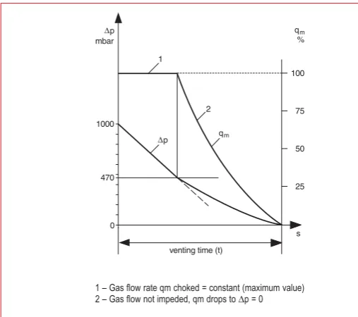
The phenomenon of choked flowmay also be observed in the viscous flow situation. It plays a part when venting and evacuating a vacuum vessel and where there are leaks.

Gas will always flow where there is a difference in pressure

Δp = (p₁– p₂) > 0. The intensity of the gas flow, i.e. the quantity of gas flowing over a period of time, rises with the pressure differential. In the case of viscous flow, however, this will be the case only until the flow velocity, which also rises, reaches the speed of sound. This is always the case at a certain pressure differential and this value may be characterized as “criti-cal”:

(1.22)

A further rise in Δp > Δp_critwould not result in any further rise in gas flow; any increase is inhibited. For air at 20,°C the gas dynamics theory reveals a critical value of

(1.23)

The chart in Fig. 1.1 represents schematically the venting (or airing) of an evacuated container through an opening in the envelope (venting valve), allowing ambient air at p = 1000 mbar to enter. In accordance with the infor-mation given above, the resultant critical pressure is

Δp_crit= 1000 ⋅(1– 0.528) mbar ≈ 470 mbar; i.e. where Δp > 470 mbar the flow rate will be choked; where Δp < 470 mbar the gas flow will decline.

p

_crit

2

1

0528

⎛ ⎝

⎜ ⎞_⎠⎟

= .

Δ

p

crit

=

−⎛ ⎝

⎜ ⎞_⎠⎟

⎡ ⎣

⎢ ⎤

⎦ ⎥

1 2

1

Molecular flow

Molecular flow prevails in the high and ultrahigh vacuum ranges. In these regimes the molecules can move freely, without any mutual interference. Molecular flow is present where the mean free path length for a particle is very much larger than the diameter of the pipe:

λ

>> d.

Knudsen flow

The transitional range between viscous flow and molecular flow is known as Knudsen flow. It is prevalent in the medium vacuum range:

λ

≈ d.

The product of pressure p and pipe diameter d for a particular gas at a cer-tain temperature can serve as a characterizing quantity for the various types of flow. Using the numerical values provided in Table III, Chapter 9, the following equivalent relationships exist for air at 20 °C:

Rough vacuum – Viscous flow

⇔

p ⋅d > 6.0 ⋅10–1_mbar_⋅_cm

Medium vacuum – Knudsen flow

⇔

6 ⋅10–1_{> p}_⋅_{d > 1.3}_⋅₁₀–2_mbar_⋅_cm

High and ultrahigh vacuum – Molecular flow

⇔

p ⋅d < 1.3 ⋅10–2_mbar_≠_cm

In the viscous flow range the preferred speed direction for all the gas mole-cules will be identical to the macroscopic direction of flow for the gas. This alignment is compelled by the fact that the gas particles are densely packed and will collide with one another far more often than with the boundary walls of the apparatus. The macroscopic speed of the gas is a

λ >

d

2

d

100

< <

λ

2

λ <

100

d

Vacuum physics

Δp mbar

qm

%

1

2

1000

qm Δp

470

0

25 50 75 100

s

venting time (t)

Fig. 1.1 Schematic representation of venting an evacuated vessel

(17)

“group velocity” and is not identical with the “thermal velocity” of the gas molecules.

In the molecular flow range, on the other hand, impact of the particles with the walls predominates. As a result of reflection (but also of desorption fol-lowing a certain residence period on the container walls) a gas particle can move in any arbitrary direction in a high vacuum; it is no longer possible to speak of ”flow” in the macroscopic sense.

It would make little sense to attempt to determine the vacuum pressure ranges as a function of the geometric operating situation in each case. The limits for the individual pressure regimes (see Table IX in Chapter 9) were selected in such a way that when working with normal-sized laboratory equipment the collisions of the gas particles among each other will predom-inate in the rough vacuum range whereas in the high and ultrahigh vacuum ranges impact of the gas particles on the container walls will predominate. In the high and ultrahigh vacuum ranges the properties of the vacuum con-tainer wall will be of decisive importance since below 10–3_{mbar there will} be more gas molecules on the surfaces than in the chamber itself. If one assumes a monomolecular adsorbed layer on the inside wall of an evacuat-ed sphere with 1 l volume, then the ratio of the number of

adsorbed particles to the number of free molecules in the space will be as follows:

at 1 mbar 10–2

at 10–6 _mbar ₁₀+4 at 10–11 _mbar ₁₀+9

For this reason the monolayer formation time τ(see Section 1.1) is used to characterize ultrahigh vacuum and to distinguish this regime from the high vacuum range. The monolayer formation time τis only a fraction of a sec-ond in the high vacuum range while in the ultrahigh vacuum range it extends over a period of minutes or hours. Surfaces free of gases can therefore be achieved (and maintained over longer periods of time) only under ultrahigh vacuum conditions.

Further physical properties change as pressure changes. For example, the thermal conductivity and the internal friction of gases in the medium vacu-um range are highly sensitive to pressure. In the rough and high vacuvacu-um regimes, in contrast, these two properties are virtually independent of pres-sure.

Thus, not only will the pumps needed to achieve these pressures in the various vacuum ranges differ, but also different vacuum gauges will be required. A clear arrangement of pumps and measurement instruments for the individual pressure ranges is shown in Figures 9.16 and 9.16a in Chapter 9.

1.5.2 Calculating conductance values

The effective pumping speed required to evacuate a vessel or to carry out a process inside a vacuum system will correspond to the inlet speed of a particular pump (or the pump system) only if the pump is joined directly to the vessel or system. Practically speaking, this is possible only in rare situ-ations. It is almost always necessary to include an intermediate piping sys-tem comprising valves, separators, cold traps and the like. All this

Vacuum physics

represents an resistance to flow, the consequence of which is that the effective pumping speed S_effis always less than the pumping speed S of the pump or the pumping system alone. Thus to ensure a certain effective pumping speed at the vacuum vessel it is necessary to select a pump with greater pumping speed. The correlation between S and S_effis indicated by the following basic equation:

(1.24)

Here C is the total conductance value for the pipe system, made up of the individual values for the various components which are connected in series (valves, baffles, separators, etc.):

(1.25)

Equation (1.24) tells us that only in the situation where C = ∞(meaning that the flow resistance is equal to 0) will S = S_eff. A number of helpful equations is available to the vacuum technologist for calculating the con-ductance value C for piping sections. The concon-ductance values for valves, cold traps, separators and vapor barriers will, as a rule, have to be determined empirically.

It should be noted that in general that the conductance in a vacuum com-ponent is not a constant value which is independent of prevailing vacuum levels, but rather depends strongly on the nature of the flow (continuum or molecular flow; see below) and thus on pressure. When using conductance indices in vacuum technology calculations, therefore, it is always necessary to pay attention to the fact that only the conductance values applicable to a certain pressure regime may be applied in that regime.

1.5.3 Conductance for piping and orifices

Conductance values will depend not only on the pressure and the nature of the gas which is flowing, but also on the sectional shape of the conducting element (e.g. circular or elliptical cross section). Other factors are the length and whether the element is straight or curved. The result is that vari-ous equations are required to take into account practical situations. Each of these equations is valid only for a particular pressure range. This is always to be considered in calculations.

a) Conductance for a straight pipe, which is not too short, of length l, with a circular cross section of diameter d for the laminar, Knudsen and mol-ecular flow ranges, valid for air at 20 °C (Knudsen equation):

(1.26) where

d = Pipe inside diameter in cm l = Pipe length in cm (l ≥ 10 d)

p₁ = Pressure at start of pipe (along the direction of flow) in mbar p₂ = Pressure at end of pipe (along the direction of flow) in mbar

p

=

p

1

+

p

2

C

d

l

p

=

135

+

4

d

l

d p

s

·

+

· ·

+

· ·

12 1

1 192

1 237

3

.

/

1 1 1 1 1

1 2 3

C C C C Cn

= + + + . . .

1

(18)

Vacuum physics

If one rewrites the second term in (1.26) in the following form

(1.26a)

with

(1.27)

it is possible to derive the two important limits from the course of the func-tion f (d ·

p

–):

Limit for laminar flow

(d ·–

p

> 6 ·10–1_mbar_·_cm):

(1.28a)

Limit for molecular flow

(d ·p–< 10–2_mbar_·_{cm) :}

(1.28b)

In the molecular flow region the conductance value is independent of pressure!

The complete Knudsen equation (1.26) will have to be used in the transi-tional area 10–2_{< d}_·_p–_{< 6}_·₁₀–1_mbar_·_{cm. Conductance values for} straight pipes of standard nominal diameters are shown in Figure 9.5 (lami-nar flow) and Figure 9.6 (molecular flow) in Chapter 9. Additional nomo-grams for conductance determination will also be found in Chapter 9 (Figures 9.8 and 9.9).

b) Conductance value C for an orifice A

(A in cm2_{): For continuum flow (viscous flow) the following equations} (after Prandtl) apply to air at 20 °C where p₂/p₁= δ:

C

d

l

s

=

12 1

·

3

.

/

C

d

l

p

s

=

135

·

4

/

( )

f d p d p d p

d p

· = + · · + · · ·

+ · ·

1 203 2 10

1 237

3 2 2

.78

(

)

C

d

l

f d p

=

12 1

·

3

.

for δ≥ 0.528 (1.29)

for δ≤ 0.528 (1.29a)

and for δ≤ 0,03 (1.29b)

δ= 0.528 is the critical pressure situation for air

Flow is choked at δ< 0.528; gas flow is thus constant. In the case of mole-cular flow (high vacuum) the following will apply for air:

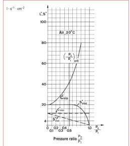
Cmol = 11,6 ·A·l ·s-1 (A in cm2₎ _(1.30) Given in addition in Figure 1.3 are the pumping speeds S*_viscand S*_mol refer-enced to the area A of the opening and as a function of δ = p₂/p₁. The equations given apply to air at 20 °C. The molar masses for the flowing gas are taken into consideration in the general equations, not shown here.

p p

crit 2

1

⎛ ⎝

⎜ ⎞

⎠ ⎟

C

A

s

visc

=

20

·

C

A

s

visc

=

20

·

1

−

δ

C A

s

visc=76 6. ·δ0.712· 1−δ0.288·₁₋_δ

Fig. 1.2 Flow of a gas through an opening (A) at high pressures (viscous flow) Fig. 1.3 Conductance values relative to the area, C*_visc, C*_mol, and pumping speed S*_viscand S*_molfor an orifice A, depending on the pressure relationship p₂/p₁for air at 20 °C.

(19)

Vacuum physics

When working with other gases it will be necessary to multiply the conduc-tance values specified for air by the factors shown in Table 1.1.

Nomographic determination of conductance values

The conductance values for piping and openings through which air and other gases pass can be determined with nomographic methods. It is pos-sible not only to determine the conductance value for piping at specified values for diameter, length and pressure, but also the size of the pipe diam-eter required when a pumping set is to achieve a certain effective pumping speed at a given pressure and given length of the line. It is also possible to establish the maximum permissible pipe length where the other parameters are known. The values obtained naturally do not apply to turbulent flows. In doubtful situations, the Reynolds number Re (see Section 1.5.) should be estimated using the relationship which is approximated below

(1.31)

Here q_pV= S ·p is the flow output in mbar l/s, d the diameter of the pipe in cm.

A compilation of nomograms which have proved to be useful in practice will be found in Chapter 9.

1.5.4 Conductance values for other elements

Where the line contains elbows or other curves (such as in right-angle valves), these can be taken into account by assuming a greater effective length l_effof the line. This can be estimated as follows:

(1.32)

Where

l_axial : axial length of the line (in cm) l_eff : Effective length of the line (in cm) d : Inside diameter of the line (in cm) θ : Angle of the elbow (degrees of angle)

l_eff=l_axial+ · d

°· 133

180

. θ

Re =

15

·

q

d

pV

The technical data in the Leybold catalog states the conductance values for vapor barriers, cold traps, adsorption traps and valves for the molecular flow range. At higher pressures, e.g. in the Knudsen and laminar flow ranges, valves will have about the same conductance values as pipes of corresponding nominal diameters and axial lengths. In regard to right-angle valves the conductance calculation for an elbow must be applied. In the case of dust filters which are used to protect gas ballast pumps and roots pumps, the percentage restriction value for the various pressure lev-els are listed in the catalog. Other components, namely the condensate separators and condensers, are designed so that they will not reduce pumping speed to any appreciable extent.

The following may be used as a rule of thumb for dimensioning vacuum lines: The lines should be as short and as wide as possible.They must exhibit at least the same cross-section as the intake port at the pump. If particular circumstances prevent shortening the suction line, then it is advisable, whenever this is justifiable from the engineering and economic points of view, to include a roots pump in the suction line. This then acts as a gas entrainment pump which reduces line impedance.

Table 1.1 Conversion factors (see text)

Gas (20 °C) Molecular flow Laminar flow

Air 1.00 1.00

Oxygen 0.947 0.91

Neon 1.013 1.05

Helium 2.64 0.92

Hydrogen 3.77 2.07

Carbon dioxide 0.808 1.26

Water vapor 1.263 1.73

(20)

2.

Vacuum generation

2.1.

Vacuum pumps: A survey

Vacuum pumps are used to reduce the gas pressure in a certain volume and thus the gas density (see equation 1.5). Consequently consider the gas particles need to be removed from the volume. Basically differentiation is made between two classes of vacuum pumps:

a) Vacuum pumps where – via one or several compression stages – the gas particles are removed from the volume which is to be pumped and ejected into the atmosphere (compression pumps). The gas particles are pumped by means of displacement or pulse transfer.

b) Vacuum pumps where the gas particles which are to be removed condense on or are bonded by other means (e.g. chemically) to a solid surface, which often is part of the boundary forming volume itself. A classification which is more in line with the state-of-the-art and practical applications makes a difference between the following types of pumps, of

which the first three classes belong to the compression pumps and where the two remaining classes belong to the condensation and getter pumps: 1. Pumps which operate with periodically increasing and decreasing pump

cham-ber volumes (rotary vane and rotary plunger pumps; also trochoid pumps)

2. Pumps which transport quantities of gas from the low pressure side to the high pressure side without changing the volume of the pumping chamber (Roots pumps, turbomolecular pumps)

3. Pumps where the pumping effect is based mainly on the diffusion of gases into a gas-free high speed vapor jet (vapor pumps)

4. Pumps which pump vapors by means of condensation (condensers) and pumps which pump permanent gases by way of condensation at very low temperatures (cryopumps)

5. Pumps which bond or incorporate gases by adsorption or absorption to surfaces which are substantially free of gases (sorption pumps). A survey on these classes of vacuum pumps is given in the diagram of Table 2.1.

Vacuum generation

Adsorption pump Fluid entrainment

vacuum pump

Ejector vacuum pump

Liquid jet vacuum pump

Gas jet vacuum pump

Vapor jet vacuum pump

Diffusion pump

Self-purifying diffusion pump

Fractionating diffusion pump

Diffusion ejector pump Drag

vacuum pump

Gaseous ring vacuum pump

Turbine vacuum pump

Axial flow vacuum pump

Radial flow vacuum pump

Molecular drag vacuum pump

Turbomolecular pump Rotary

vacuum pump

Liquid sealed vacuum pump

Liquid ring vacuum pump

Rotary vane vacuum pump

Multiple vane vacuum pump

Rotary piston vacuum pump

Rotary plunger vacuum pump

Dry compressing vacuum pump

Roots vacuum pump

Claw vacuum pump

Scroll pump Reciprocating

positive displacement vacuum pump

Diaphragm vacuum pump

Piston vacuum pump

Ion transfer vacuum pump

Getter pump

Bulk getter pump

Sublimation pump

Getter ion pump

Evaporation ion pump

Sputter-ion pump

Cryopump

Condenser

Vacuum pump (Operating principle)

Kinetic vacuum pump Gas transfer

vacuum pump Positive displacement

vacuum pump

Entrapment vacuum pump

(21)

Vacuum generation

2.1.1 Oscillation displacement vacuum pumps

2.1.1.1 Diaphragm pumps

Recently, diaphragm pumps have becoming ever more important, mainly for environmental reasons. They are alternatives to water jet vacuum pumps, since diaphragm pumps do not produce any waste water. Overall, a diaphragm vacuum pump can save up to 90 % of the operating costs compared to a water jet pump. Compared to rotary vane pumps, the pumping chamber of diaphragm pumps are entirely free of oil. By design, no oil immersed shaft seals are required. Diaphragm vacuum pumps are single or multi-stage dry compressing vacuum pumps (diaphragm pumps having up to four stages are being manufactured). Here the circumference of a diaphragm is tensioned between a pump head and the casing wall (Fig. 2.1). It is moved in an oscillating way by means of a connecting rod and an eccentric. The pumping or compression chamber, the volume of which increases and decreases periodically, effects the pumping action. The valves are arranged in such a way that during the phase where the volume of the pumping chamber increases it is open to the intake line. During compression, the pumping chamber is linked to the exhaust line. The diaphragm provides a hermetic seal between the gear chamber and the pumping chamber so that it remains free of oil and lubricants (dry compressing vacuum pump). Diaphragm and valves are the only components in contact with the medium which is to be pumped. When coating the diaphragm with PTFE (Teflon) and when manufacturing the inlet and exhaust valves of a highly fluorinated elastomer as in the case of the DIVAC from LEYBOLD, it is then possible to pump aggressive vapors and gases. It is thus well suited for vacuum applications in the chemistry lab. Due to the limited elastic deformability of the diaphragm only a

comparatively low pumping speed is obtained. In the case of this pumping principle a volume remains at the upper dead center – the so called “dead space” – from where the gases can not be moved to the exhaust line. The quantity of gas which remains at the exhaust pressure expands into the

expanding pumping chamber during the subsequent suction stroke thereby filling it, so that as the intake pressure reduces the quantity of inflowing new gas reduces more and more. Thus volumetric efficiency worsens

continuously for this reason. Diaphragm vacuum pumps are not capable of attaining a higher compression ratio than the ratio between “dead space” and maximum volume of the pumping chamber. In the case of single-stage diaphragm vacuum pumps the attainable ultimate pressure amounts to approximately 80 mbar. Two-stage pumps such as the DIVAC from LEYBOLD can attain about 10 mbar (see Fig. 2.2), three-stage pumps can attain about 2 mbar and four-stage diaphragm pumps can reach about 5·10-1_mbar.

Diaphragm pumps offering such a low ultimate pressure are suited as backing pumps for turbomolecular pumps with fully integrated Scroll stages (compound or wide range turbomolecular pumps, such as the

TURBOVAC 55 from LEYBOLD). In this way a pump system is obtained which is absolutely free of oil, this being of great importance to

measurement arrangements involving mass spectrometer systems and leak detectors. In contrast to rotary vane pumps this combination of pumps for leak detectors offers the advantage that naturally no helium is dissolved in the diaphragm pump thereby entirely avoiding a possible build up of a helium background.

2.1.2 Liquid sealed rotary displacement pumps

2.1.2.1 Liquid ring pumps

Due to the pumping principle and the simple design, liquid ring vacuum pumps are particularly suited to pumping gases and vapors which may also contain small amounts of liquid. Air, saturated with water vapors or other gases containing condensable constituents, may be pumped without problems. By design, liquid ring pumps are insensitive to any contamination

(1) Casing lid (2) Valves (3) Lid (4) Diaphragm disk

(5) Diaphragm (6) Diaphragm support disk (7) Connecting rod (8) Eccentric disk

Fig. 2.1 Schematic on the design of a diaphragm pump stage (Vacuubrand) Fig. 2.2 Principle of operation for a two-stage diaphragm pump (Vacuubrand) Opening and closing of the valves, path and pumping mechanism during four subsequent phases of a turn of the connecting rod (a-d)

a )

b)

c )

d)

1st stage 2nd stage

(22)

which may be present in the gas flow. The attainable intake pressures are in the region between atmospheric pressure and the vapor pressure of the operating liquid used. For water at 15 °C it is possible to attain an operating pressure of 33 mbar. A typical application of water ring vacuum pumps is venting of steam turbines in power plants. Liquid ring vacuum pumps (Fig. 2.3) are rotary displacement pumps which require an operating liquid which rotates during operation to pump the gas. The blade wheel is arranged eccentrically in a cylindrical casing. When not in operation, approximately half of the pump is filled with the operating fluid. In the axial direction the cells formed by the blade wheel are limited and sealed off by “control discs�

Vacuum Fundamentals Lybold

Kat.-Nr. 199 90

Preface

3. Vacuum measurement, monitoring, control and regulation . . . .76

1. Vacuum physics Quantities, their symbols, units of measure and definitions . . . .9

2. Vacuum Generation . . . .19

Table of Contents

4. Analysis of gas at low pressures using

5 Leaks and their detection . . . .110

6 Thin film controllers and control units with quartz oscillators . . . .125

7 Application of vacuum technology for coating techniques . . . .133

Table of Contents

8 Instructions for vacuum equipment operation . . . .139

9. Tables, formulas, nomograms, diagrams and symbols . . .147

10. The statutory units used in vacuum technology . . . .171

Table of Contents

11. National and international standards and recommendations particularly relevant

Vacuum physics

Absolute pressure pabs

Saturation vapor pressure ps

Ultimate pressure pend

Working pressure pW

The ideal gas law

Vacuum physics

Volumetric flow (flow volume) qv

Vacuum physics

Pump throughput qpV

Vacuum physics

monolayer formation time

Vacuum physics

Gas laws and models

Summary of the most important gas laws (continuum theory)

van der Waals’ Equation

1.3.2 Kinetic gas theory

Vacuum physics

Model concepts and basic assumptions:

Ideal gas law (derived from the kinetic gas theory)

The pressure ranges in vacuum technology

Types of flow and conductance

Viscous or continuum flow

Molecular flow

Rough vacuum – Viscous flow

Vacuum physics

1.5.2 Calculating conductance values

1.5.3 Conductance for piping and orifices

Vacuum physics

Limit for laminar flow

Vacuum physics

Nomographic determination of conductance values

1.5.4 Conductance values for other elements

Vacuum generation

Vacuum generation

Kinetic vacuum pump Gas transfer

Vacuum generation

2.1.2 Liquid sealed rotary displacement pumps